August 24, 2026
LBNL-152E
Planar Graphs On The World Sheet: The Hamiltonian Approach 11 1 This work was supported by the Director, Office of Science, Office of Basic Energy Sciences, of the U.S. Department of Energy under Contract DE-AC02-05CH11231.
Korkut Bardakci
Department of Physics
University of California at Berkeley
and
Theoretical Physics Group
Lawrence Berkeley National Laboratory
University of California
Berkeley, California 94720
The present work continues the program of summing planar Feynman graphs on the world sheet. Although it is based on the same classical action introduced in the earlier work, there are two important new features: Instead of the path integral used in the earlier work, the model is quantized using the canonical algebra and the Hamiltonian picture. The new approach has an important advantage over the old one: The ultraviolet divergence that plagued the earlier work is absent. Using a family of projection operators, we are able to give an exact representation on the world sheet of the planar graphs of both the theory, on which most of the previous work was based, and also of the theory. We then apply the mean field approximation to determine the structure of the ground state. In agreement with the earlier work, we find that the graphs of theory form a dense network (condensate) on the world sheet. In the case of the theory, graphs condense for the unphysical (attractive) sign of the coupling, whereas there is no condensation for the physical (repulsive) sign.
1. Introduction
Several years ago, the present author and Charles Thorn initiated a program for summing planar graphs of a given field theory [1,2]. The model most intensively studied so far is the theory, although there have been extensions to more physical theories as well [3]. The starting point of this program is the observation, due to G.’t Hooft, that planar graphs of theory, expressed in light cone variables, can be represented on the world sheet [4]. It was shown in [1] that this representation can be derived from a local world sheet field theory. This reformulation opened the way for the application of various field theory techniques to the summation of planar graphs.
The present article can be thought of as a follow up to an earlier work on the same subject [5], which we review in section 2. Although there is quite a bit of overlap between the present work and [5], there are also significant differences. The part of the earlier work that forms the starting point of this paper is the path integral, based on a suitable action, which automatically sums the planar graphs of massless model. Here, we also start with same world sheet fields and the same action as in [5] (eq.(7)). However, as it stands, this path integral has two defects: The factor of in the propagator (eq.(1)) is missing and, more seriously, it suffers from both infrared and ultraviolet divergences. In [5], the infrared divergence was regulated by discretizing one of the coordinates of the world sheet. In section 2, we point out that this discretization is the same as compactifying the light cone coordinate on a circle. This type of compactification was first introduced in connection with the M theory [6,7]; it can be viewed as an infinite boost of more standard compactification of a spacelike direction. We take the point of view that this is not really a serious problem, since, after all, the compactified model is interesting and perfectly consistent on its own right. How to decompactify it is an interesting question which will be left for future research.
The ultraviolet divergence has a more complicated origin. As explained in section 2, it is caused by the integration over an auxilliary field on the world sheet. The solution to this problem proposed in [5] was to introduce a Gaussian convergence factor (eq.(8)). This cures the original divergence, but unfortunately, it introduces a new ultraviolet divergence, which has to be regulated by a cutoff. The existence of this cutoff, which is really an ad hoc modification of the theory, has been a stumbling block to the further development of the program, since it is not clear how to get rid of it. The standard idea of renormalization does not seem to be applicable here. The main result of this article is to show that when the model is quantized correctly, the original divergence is absent. Therefore, there is no need for the Gaussian convergence factor, and consequently, the ultraviolet divergence which resulted from it is also avoided. This is the essential improvement introduced here over the earlier work.
In view of the problem discussed above, to what extent can we trust the action given by (7)? At the end of section 2, we argue that we can trust it as a classical action: it reproduces the correct equations of motion, eqs.(2) and (3), for the world sheet fields. Quantizing it by the path integral based on this action is problematic since, as we have already pointed out, it results in a divergent answer.
To overcome this difficulty, we take a different, and we believe, a better founded route to quantization. Following the well known prescription of elementary quantum mechanics, we read off the canonical variables and the Hamiltonian from the classical theory, and then impose the standard canonical commutation relations. This defines the dynamics in the Heisenberg picture. We argue in sections 3 and 4 that the model consists of a finite number of degrees of freedom, and therefore it cannot have any ultraviolet divergence, whose existence requires an infinite number of degrees of freedom. As a check, the ground state energy, computed in the mean field approximation in section 6, comes out finite.
We will carry out the program described above in two steps. First, the non-interacting model is treated in section 3. In this simple case, the quantized Hamiltonian is easy to construct; however, to express it in a compact form, we found it necessary to introduce a family of projection operators. These operators and their close relatives later play an essential role in the incorporation of the mising factor and in the generalization to the model. The idea behind these projection operators was already present in reference [5]; but there they were introduced in the context of the mean field approximation. Here they are given a precise formulation independent of any approximation scheme.
In the second step of the program, carried out in section 4, the interaction term is taken into account. Rather than try to do this directly in the Heisenberg picture, it is more convenient to take a detour and do the quantization in the interaction representation. The advantage of this approach is that in between the interaction times, fields propagate freely, and the free Hamiltonian and its quantization developed in the previous section can be taken over without any change. Also, an extra term induced by the interaction can be computed with relative ease.
So far, we have been working in the Heisenberg picture based on the Hamiltonian; but once we have the full Hamiltonian, we can reconstruct the corresponding action, (25), through the standard Legendre transformation. Since the action depends on both the coordinates and their conjugate momenta, to compare it to a path integral based on an action like eq.(4), which depends only on the coordinates (fields), one has to carry out the integration over the momenta. In most practical cases, the dependence on the momenta is quadratic, so the integration can be explicitly done. In contrast, here the momentum dependence is more complicated, and doing the momentum integration is really not feasible. Therefore, we conclude that the action of equation (4) makes sense only classically and it cannot be used directly in the path integral. One has either to forego the path integral entirely and instead work with the Hamiltonian, as we are doing here, or try to work with the phase space version of the path integral. This point is discussed more fully at the end of section 4.
In section 5, the missing factor is incorporated in the definition of the interaction vertex. This is done by means of a projection operator, closely related to the one already used in the construction of the free Hamiltonian. With this missing step finally in place, we have an exact reformulation of the planar theory in terms of a Hamiltonian on the world sheet.
Needless to say, although this Hamiltonian is exact, it is also quite complicated, and one needs a manageable approximation scheme. In section 6, we introduce the mean field approximation scheme, which was already used extensively in the past work [2,5]. This approximation scheme is most conveniently formulated in terms of the composite field , defined by eq.(5): It simply amounts to replacing by its ground state expectation value . The ground state energy is then computed as a function of , and minimizing it determines the value of . This is pretty much along the lines of the standard effective potential calculation of the ground state [8].
In section 6, we carry out this calculation and find a non-zero value for , which implies the following interesting structure for the world sheet. The world sheet consists of two parts: The bulk, where the field propagates freely, and the boundaries, marked by solid lines in Fig.1, where Dirichlet boundary conditions are imposed (eq.(3)). The field measures the density of the solid lines (boundaries) on the world sheet. A non-zero ground state expectation value corresponds to a finite density of solid lines, which we identify with a new phase of the model, and call it the condensate phase. In this phase, the Feynman graphs have condensed to form a dense network on the world sheet, and the dominant contribution to the ground state comes from the higher order graphs. In contrast, if is zero, the density of the solid lines tends to zero in the limit of large radius of compactification. In this phase, which we call the perturbative phase, the main contribution to the ground state comes from the lower order graphs. The calculation in section 6 shows that the condensate phase has lower ground state energy than the perturbative phase. At the end of the section, we compare the cutoff independent ground state energy with the cutoff dependent result of [5], and point out both the common features and the differences.
At this point, a natural question to ask is whether the condensation of the Feynman graphs leads to the formation of a string. The geometric intuition indeed suggests that a dense network of Feynman graphs on the world sheet should be identified with some sort of a string; in fact, this was the picture that motivated the original work on this subject [9,10]. This picture should be confirmed or disproved by determining the spectrum of the model and comparing it to the linearly rising trajectories of string theory. We hope to return to this problem in the future.
In the next section, section 7, we apply the machinery developed in the previous sections to the theory. First, we present an exact formulation of the model on the world sheet, and then we apply the mean field method to determine its ground state. For the physical sign of the coupling constant, corresponding to a stable theory, nothing interesting happens: It is the perturbative phase that is energetically favored. On the other hand, for the “wrong” sign of the coupling constant, corresponding to an unstable model, the condensate phase has the lower ground state energy. We discuss a possible physical reason for this correlation between instability and condensate formation. Finally, in section 8, we summarize our conclusions and suggest some directions for future research.
2. The World Sheet Action
In this section, we briefly review the the world sheet action, developed in references [1,2,5], for the planar graphs of theory in dimensions. Starting with the world sheet parametrized by the light cone variables
a general planar Feynman graph can be represented by a bunch of horizontal solid lines (Fig.1).

The n’th solid line carries a transverse momentum , and two adjacent lines n and n+1, represent the light cone propagator
| (1) |
where . The interaction takes place at the beginning and the end of each line, where a factor of g, the coupling constant, is inserted [1,4].
We remind the reader that the planar model we are studying is the large limit of a field theory with the interaction
where the field is an Hermitian matrix. As ’t Hooft showed [5], in this limit, each planar graph appears once and once only. There are no local symmetry factors, such as the well known factor of associated with the one loop contribution to the propagator of an ordinary theory, where is not a matrix. There may be, however, global symmetry factors associated with special configurations of momenta of the external lines. In this paper, we are only considering generic graphs with no global symmetries, and we are focusing exclusively on the dynamics in the bulk, represented by the Hamiltonian.
In the case , the light cone Feynman rules sketched above can be reproduced by a field theory that lives on the world sheet. To keep things simple, we will study the massless model exclusively in this work, although using the tools we are going to develop, one can easily introduce a finite mass. Here, we briefly describe the equivalent field theory, and refer to [5] for the detailed derivations. The transverse momenta , originally defined only on the solid lines, can be promoted to local fields over the whole world sheet. The solid lines form the world sheet boundaries, and satisfies the equation
| (2) |
in the bulk, and the Dirichlet condition
| (3) |
on the boundaries. With the help of a Lagrange multiplier field , both the equations of motion and the boundary conditions are incorporated in the following action [5]:
| (4) |
where a dot represents derivative with respect to and a prime the derivative with respect to . The coordinate is compactified by imposing periodic boundary conditions at and , where is the total component of the momentum entering the graph. The field is a delta function on the boundaries and vanishes in the bulk: It is inserted to ensure that the Dirichlet condition (3) is imposed only on the boundaries.
In the functional integral, one has to integrate not only over and , but also over the locations and the lengths of the solid lines. This is best accomplished by introducing a two component fermion field , , and its adjoint , and setting
| (5) |
The action for the fermions is 22 2 Here we are using the letter for both the world sheet coordinate and also for Pauli matrices to be sandwiched between and . Hopefully, there should be no confusion about the dual use of this letter.
| (6) |
So far, we have been treating both and as continuous variables. However, as explained in the introduction, to avoid infrared divergences, we are going to compactify the lightcone coordinate at a radius . This is equivalent to discretizing the coordinate into segments of length , where . The discretization also makes it easy to visualize what is going on on the world sheet. As pictured in Fig.2, the world sheet consists of horizontal dotted and solid lines, spaced at distance apart.
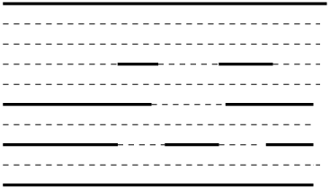
The boundaries are marked by the solid lines, associated with the component of the fermion, and the bulk is filled with the dotted lines, associated with the component. The first term in eq.(6) represents the free propagation of the fermion, tracing a solid or dotted line, and the second term, which converts a dotted line into a solid one or vice versa, represents the interaction. We note that there are some extra unwanted states in the fermionic Hilbert space; they can be eliminated by truncating it to states singly occupied at each value of . This can be done consistently since fermion number is locally conserved. Integrating over the fermion field is then the same as summing over the location and the length of the boundaries.
The integrals over in eqs.(4,6) are in reality finite sums with terms:
In order not to complicate the notation, from time to time, we will still write an integral over , although in reality it is a discrete sum. Wherever possible, we will simplify the algebra by taking to be large, but always finite. For example, when integrating over ((9,10)), we used the large (small ) approximation. This is not essential, but it avoids unnecessary complications. In contrast to , the time coordinate will remain continuous.
It is now natural to identify
| (7) |
as the candidate for the total action. There are, however, two problems
with this choice:
a) The exponential part of the propagator in eq.(1) is correctly
reproduced, but the prefactor
is missing. This will be corrected in
section 5.
b) A more serious drawback is that, as it stands, the functional
integral over is divergent. This is because lives
effectively only on the solid lines:
The integrand is
independent of in the bulk (on the dotted lines). Consequently,
the integrations over those which live in the bulk are divergent.
The solution to this problem, proposed in reference [5], was to introduce an additional term given by
where is a parameter and is defined by
| (8) |
and it is complimentary to : It vanishes on the solid lines and provides a Gaussian cutoff for the functional integral on the dotted lines. The divergence mentioned above is therefore cured; but unfortunately, it is replaced by a new divergence: The action (8) is ultraviolet divergent and needs a cutoff. One way to see this is to notice that in the bulk, introduces a mass term for the field , but there is no corresponding kinetic energy term in the action. A field theory with only a mass term in the action has a constant, momentum independent propagator and therefore it is ultraviolet divergent. In reference [5], the model studied was an ultraviolet regulated theory based on the action
Apart from the drawback of the need for an ultraviolet cutoff, the introduction of a new parameter suggests that this model may no longer be the original theory but some modification of it.
In the present work, we wish to avoid introducing any spurious cutoff or modifying the original theory in any way. Therefore, our starting point will simply be eq.(4), without the additional term . We then face the problem of a divergent functional integral mentioned above.
The solution to this problem, as we shall soon see, is to adopt the
Hamiltonian formulation. We would like to emphasize that, independent
of the divergence problems, the Hamiltonian approach is the correct
approach. Our reasoning goes as follows:
a) The action of eq.(4) is correct classically. The classical equations
derived from it are precisely the bulk equations (2) and the boundary
conditions (3). The solution to these equations reproduces any arbitrary
light cone Feynman graph for fixed boundaries as a function of the
momenta flowing through these boundaries.
b) This takes care of the “classical” part of the problem. The
“quantum” part is the integration over the momenta and the positions
of the boundaries. Keeping the boundaries fixed for the moment, there
are two options for quantization: The first option is to
plug in the action (4) in
the exponent and integrate functionally over the fields. The fundamental
problem with this choice is that we do not know a priori what
measure to use in the functional integral.
c) The second option is to take the standard route to quantization:
Read off the canonical variables from the classical action and impose
the canonical commutation relations and finally construct the Hamiltonian.
This approach, which we are going to follow,
is the more fundamental one. Apart from possible operator ordering
ambiguities, which are not present in this case, given the classical
action, the corresponding quantum Hamiltonian
is uniquely determined. If so desired, from the Hamiltonian in operator
form, one can derive the corresponding path integral as Feynman did and
thereby deduce the integration measure.
d) In the free theory, the dotted and solid lines are eternal, but the
interaction converts a dotted line into a solid one and vice versa.
This is taken care of by introducing fermions on the world sheet.
(see eq.(6)).
This formalism was extensively developed in the earlier work [2,5], and it
is applicable here without any change.
e) Although we find our canonical quantization of the classical action
quite compelling, it is still desirable to demonstrate directly that
the Hamiltonian formalism correctly reproduces the light cone
perturbation series on the world sheet. We sketch such a direct
argument at the end of section 5.
3. The Hamiltonian For The Free Theory
Rather than dealing with the interacting theory in its full complexity, it is much easier to solve the problems discussed in the last section in the context of the perturbation expansion in powers of . The strategy is to first construct the Hamiltonian for the non-interacting model, and then include the interaction by going over to the interaction representation. The starting point is the action of eq.(7), with . Since there is no interaction, the solid and dotted lines are eternal, and the world sheet configuration, being time independent, is well suited for the Hamiltonian description. Let us first consider a particular graph with eternal solid lines, that is with lines with no beginning or end, located at , where runs from to . They are ordered according to increasing , with iff . The action can then explicitly be written as
| (9) |
For this simple case, it is easy to avoid the divergent functional integrals mentioned earlier. The above action depends only on , the Lagrange multipliers associated with the solid lines. The divergence comes about if one introduces additional unneeded ’s located on the dotted lines and integrates over them. Therefore, if we agree to integrate only over these that live on the solid lines, there is no longer any problem. However, this action has a serious shortcoming: It is only applicable to a particular graph with given number of solid lines located at specified positions, and different graphs are associated with different actions. In a free theory, since the solid lines are eternal, this is not a problem, but this form of the action is very awkward to generalize to the interacting theory, where the number and positions of the solid lines can change. One could try to overcome this difficulty by attaching a to every line, solid or dotted, but as we explained earlier, one then is faced with the problem of a divergent functional integral. We shall show in what follows that both of these problems can be resolved in the Hamiltonian approach.
We take the action (9) as our starting point for the construction of a Hamiltonian. We choose , , as our canonical variables, where specify the location of the solid lines. On the other hand, the ’s are auxilliary variables; one can eliminate them in favor of the ’s through the equations of motion,
| (10) |
where we have dropped a term proportional to . This is justified for the non-interacting theory (), since the fermion fields and therefore are time independent.
The action can now be rewritten solely in terms of ’s:
| (11) |
and the momenta canonically conjugate to are:
| (12) |
Conversely, ’s can be expressed in terms of the canonical momenta by,
| (13) |
Using these equations, the Hamiltonian can be written in terms of the canonical momenta:
| (14) | |||||
The model is quantized by letting
| (15) |
It is clear that the eigenstates of momenta diagonalize the Hamiltonian, and the spectrum is a continuum starting at zero. The corresponding Hilbert space is therefore labeled by the eigenstates of the ’s associated with the solid lines, or alternatively, by the eigenstates of the conjugate momenta. The difficulty now is that each graph with a different set of lines is associated with a different Hilbert space, and it is then very awkward to deal with the interaction, which generates transitions between these Hilbert spaces. This problem can simply be avoided by starting with one master Hilbert space which includes all the possible graphs. This new Hilbert space is again spanned by the simultaneous eigenvalues of at a fixed . But are no longer restricted to the positions of the solid lines, and accordingly, is now defined over the whole discretized world sheet, including both dotted and solid lines. Although the interaction term causes transitions between solid and dotted lines, the Hilbert space remains the same.
What about the Hamiltonian? The Hamiltonian is given by eq.(14), with restricted to the positions of solid lines as before. The ’s associated with the dotted lines are not present in the Hamiltonian, and the corresponding ’s are constants of motion, fixed by the initial conditions. Since, unlike in the action formulation, there is no integration over these ’s, there is no divergence problem in the Hamiltonian formulation.
There still remains one final obstacle to surmount. Although there is now only one Hilbert space for all different graphs, there is a different Hamiltonian for each graph of the free theory. This is because the sum in (14) is restricted to the positions of the solid lines, and the location and the number of solid lines change from graph to graph. If the interaction is turned on, there will be transitions between different Hamiltonians, again an awkward situation. Fortunately, the world sheet fermion field, introduced earlier [5] and reviewed in section 2, was invented to solve just this kind of a problem. So far, in constructing the Hamiltonian, we did not need the fermions, but now they become indispensable. Recall that in eq.(14), and refer to the locations of two successive solid lines, seperated by only the dotted lines (Fig.(3)). We note that this is also the configuration for a free propagator; after all, the free Hamiltonian is nothing but a collection of free propagators. Out of the fermionic fields, we wish to construct an projection operator which automatically selects such configurations. Let us now define, for any two and , with ,
| (16) |
where and are defined by eqs.(5) and (8), and they are located at the same . We usually suppress the dependence on time coordinate , but in the definition of the Hamiltonian, for example, in eq.(18), it is understood that all fields are at the same . We recall that is one on solid lines and zero on the dotted ones, whereas is zero on the solid lines and one on the dotted ones, with
Our notation is such that , etc. refer to the positions of only the solid lines, whereas , etc. refer to the positions of both the solid and the dotted lines.
From this definition, it follows that
| (17) |
if and only if two solid lines are located at and , seperated only by dotted lines, as in Fig.3.

We recall that the Hamiltonian (14) receives contribution only from these configurations, and for all other configurations, is zero. With the aid of this projection operator, eq.(14) can be rewritten as
| (18) |
where, the sum over and are unrestricted.
To the above Hamiltonian, we have to add the Hamiltonian for the fermion field. But in the non-interacting theory, with , and the fermionic Hamiltonian is zero. We can now quantize the bosonic sector as in eq.(15) and the fermionic sector by imposing the standard anticommutation relations. As explained in section 2, we also impose the constraint that fermion number at each site is always one. has then two possible eigenvalues for each : labeling solid lines and , labeling dotted lines. The Hilbert space, being a superposition of these possibilities, represents all free graphs, with all possible combinations of eternal solid and dotted lines. After quantization, becomes a master Hamiltonian operating in this Hilbert space, and the problems discussed earlier, involving a multitude of Hamiltonians and Hilbert spaces, are resolved. In the next section, we will generalize the present treatment to the interacting theory.
4. The Hamiltonian For The Interacting Theory
It may at first appear that the Hamiltonian of the interacting theory is the Hamiltonian of the free theory, plus the interaction term
This is not, however, the end of the story; the inclusion of interaction presents a new problem: We recall that when was eliminated in favor of through the equations of motion (10), there was a step that involved integration by parts of the time derivative in the action (4):
| (19) |
In deriving eq.(9), the term proportional to on the right hand side of this equation was dropped, since in the free theory, is time independent. In the interacting theory, this is no longer the case. Notice that this term is only non-zero at the points where transitions between the solid and dotted lines take place, and therefore it can be thought of as part of the interaction. One can see this explicitly by transforming the fermion field by
Under this transformation, the fermion kinetic energy transforms according to
| (20) |
and the unwanted term, , cancels between eqs.(19) and (20). All the other terms in the action are unchanged, except for the interaction term
| (21) |
This is then the new interaction term that has to be added to the free Hamiltonian . The resulting total Hamiltonian is, however, difficult to handle as it stands. For one thing, we would like to eliminate the auxilliary field in favor of and , as we did in the case of the free theory. But since the equations of motion for are now non-linear, this can no longer be done explicitly. Also, such a complicated theory is difficult to quantize directly. Both of these problems can be overcome by quantizing the model in the interaction representation. For the convenience of the reader, in the next paragraph, we briefly describe the interaction representation, as it is needed for the problem at hand.
Consider the operator responsible for the transition from the initial states at to final states at , and expand it in powers of . The n’th term in the perturbation expansion of this operator can be written as
where T stands for time ordering. The important point is that the fields that appear in the definition of are all free fields: For example, and evolve according to (eq.(18)), and satisfy the canonical algebra (15).
This still leaves the question of what to do with . Making use of the interaction picture, we will show that one can set
| (22) |
in , where is the freely propagating momentum conjugate to , introduced in section 3. We have already established this relation for the free theory, but only on solid lines (eq.(12)). We are therefore entitled to use it in the interaction picture, provided that the that appears in is located on a solid line. However, as we have argued earlier, the interaction takes place at the transition point between solid and a dotted lines, and to complicate matters, it can easily be shown from the equations of motion that is discontinuous at this point. This ambiguity is resolved by noticing that we are dealing with an end point contribution coming from the partial integration with respect to in (19). Consequently, the in question is located either at the beginning or the end of a solid line. We can therefore use (22) and rewrite the interaction Hamiltonian in the interaction representation as
| (23) |
Now that the interaction is written in terms of the canonical coordinates and momenta, it is possible to exit from the interaction representation and go back to the Hamiltonian picture by setting
| (24) |
where is given by (18) and by (23), and
Of course, the fields in the Hamiltonian picture are no longer free fields. Instead, they satisfy the equations of motion generated by the full interacting Hamiltonian. The main purpose of the detour via the interaction representation was to justify the replacement (22).
So far we have adopted the Hamiltonian approach, but we can now easily construct the action corresponding to , through the well known relation,
| (25) |
Since is defined over the phase space, the independent variables of integration in the corresponding functional integral are both and . Although we shall not need this action in the rest of this work, it is of some interest to compare it with eq.(4), our starting point, to see how it avoids the problem of the divergent functional integration. The crucial difference is that unlike in (25), where both the coordinates and the momenta are independent variables of integration, the functional integration in (4) is over only .
To see what is going on more clearly, we imagine carrying out the functional integral over the fermion field. The result is a sum over functional integrals, each associated with a different set of solid lines (see the discussion following eq.(15)). Consider now a typical term in this sum. The Hamiltonian depends only on the ’s that are located on the solid lines; the ’s that live on the dotted lines are absent. We recall that the functional integral over action (4) was divergent because that action was independent of the variables located at the dotted lines. In contrast, the above action still depends on those momenta through the first term on the right. Integrating over them gives the equations
| (26) |
for only those located at the dotted lines. As we have already seen earlier, the field is constrained to be independent on the dotted lines, and the corresponding momenta act as Lagrange multipliers enforcing this constraint.
We would like to stress that the form of the action where both the coordinates and the momenta appear as independent variables is more fundamental: That is the form that comes out of the usual derivation of the path integral. One can then pass to the coordinate version of the path integral by integrating over the momenta. This integration is usually easy to do since the dependence on the momenta is quadratic. However, in this case, the action (25) is not quadratic in the momenta; as we have just seen, the dependence on some of the momenta is in fact linear. Integration over these momenta resulted in the constraints (26), which are missing in the formulation based on (4). Alternatively, one may try to impose these constraints by hand, but since they change depending on the location of the dotted lines, there does not seem to be any practical way of doing it. We conclude that there is no practical alternative to the phase space form of the action; the form of the action in terms of coordinates only that was used [5] resulted in an ill defined path integral.
5. Vertex Correction
We pointed out earlier that the world sheet theory we have so far does not reproduce the prefactor in the propagator (eq.(1)). This problem was addressed in [5] in the context of the mean field approximation. Here, using the projection operator technique, we will incorporate this factor into the Hamiltonian.
Although originally the factor was part of the propagator, it turns out that it is more convenient to associate with the vertices. This is done by attaching it either to the beginning or the end of the propagator, and then transferring to the vertex located at that position. Consider the two basic vertices pictured in Fig.4 a,b.

In the first one, the vertex, a dotted line turns into a solid one, and in the other, the vertex, the reverse takes place. The solid lines are labeled as 1,2 and 3, as shown in the figure, and the propagators are labeled by the corresponding pair of indices, 12, 23 and 13 respectively. Let us call the extra factor to be attached to the first vertex and the factor that goes with the second vertex . The only thing that is fixed is their product:
| (27) |
and one is free to choose one of them arbitrarily, so long as the product satisfies the above relation. We make the natural symmetric choice 33 3 This choice is different from the one in reference [5].
| (28) |
which simplifies the resulting algebra.
We are now ready to combine the ’s with in order to supply the missing factors. Defining
| (29) |
we can , schematically, rewrite the full interaction Hamiltonian, incorporating the factors, in the following form:
| (30) |
In this equation, is a projection operator which is inserted to automatically choose the correct vertex configurations. By this, we mean the following: Both vertices in Fig.4 consist of three propagators meeting at a point, and each propagator consists of two solid lines seperated only by dotted lines. The correct vertex configuration is chosen by attaching to the propagator bounded by the solid lines 1 and 3 in Fig.4. This operator should be unity when the two solid lines are seperated by only dotted lines, and zero otherwise. We already faced exactly the same problem in deriving eq.(18), and we could use here the same projection operator, . It is, however, more convenient to define a slightly different operator:
| (31) |
The relation between the two projection operators is,
We will later see why is better suited for the later computations.
Eq.(30) can now be rewritten in a more explicit form:
| (32) |
where are the coordinates of the lines 1,2 and 3 in Fig.4. Notice that the denominators in this expression never vanish: The distance between the coordinates is at least , the unit of the lattice spacing. A possible infrared divergence is therefore avoided by the compactification of the coordinate at radius (see the discussion following eq.(6)).
To the above expression for the interaction Hamiltonian, one has to add the free Hamiltonian (eq.(18)), to arrive at the total Hamiltonian
We would like to emphasize that in this final form, the Hamiltonian is exact: Nothing has been omitted and as yet, no approximations have been made. If so desired, one could also go over to the path integral formulation through eq.(25). Of course, as would be expected, the expression for is quite complicated; for example, it is non-local in . However, it is local in the time coordinate , which makes the Hamiltonian formulation possible. Of course, one cannot hope to make progress without some approximation. In the next section, we will see that a great simplification results when one applies the mean field approximation; for example, one can determine the ground state of the model. Independent of any approximation, however, one thing should be clear: We have already seen above that there is no infrared divergence. Since what we have here is a quantum mechanical system with finite degrees of freedom, and there can also be no ultraviolet divergence. We therefore have a perfectly finite model. In the next section, we will verify this in the mean field approximation.
Before closing this section, we would like to demonstrate directly that the Hamiltonian formalism we have developed correctly reproduces the light cone Feynman graphs on the world sheet. Starting with the free Hamiltonian of eq.(14), we will show that it generates the free theory on the world sheet. Using eq.(12), we can make the replacement (eq.(22)),
on the solid lines, and note that, the time evolution operator
generates a collection of free propagators (eq.(1)), with solid lines as boundaries, without, however, the prefactor and for . But since the free theory is nothing but the collection of free propagators, this completes the demonstration.
Next, consider the interaction, which causes transitions between solid and dotted lines. The vertices responsible for these transitions are represented by the term
in the fermionic part of the Hamiltonian. The missing prefactor of the propagators can be incorporated into these vertices (see eq.(32)). The use of world sheet fermions as a tool for building interaction vertices was fully developed in references [2,5] and reviewed to some extent in the preceding sections. We therefore conclude that the interacting theory is also correctly reproduced by the Hamiltonian approach.
6. The Mean Field Approximation
The mean field approximation is a statistical approximation scheme which has been long in use in both field theory and many body physics with varying degree of success. In the context of the problem at hand, the basic idea is to replace the operator (eq.5) by its ground state expectation value :
| (33) |
To do this systematically, it is convenient first to promote to be an independent field by adding the term
| (34) |
to the action, where is a Lagrange multiplier field. An alternative approach, which we will not pursue and which gives the same results obtained here, is to bosonize the fermions. We can then in principle compute the ground state energy as a function of after integrating over the other fields. is then the classical field configuration that minimizes this energy.
Originally, being a composite of the fermions, could only take on the values 0 and 1; after being promoted to an independent field, and hence can take on any value between 0 and 1. There is also a statistical interpretation, derivable from the Euclidean version of the path integral. Remembering that corresponds to a solid line and to a dotted line, is then the probability of finding a solid line at a given location. In general, could depend on the coordinates and ; however, with the boundary conditions we have chosen (see the discussion following eq.(4)), it is natural to assume that the ground state of the system is translationally invariant in both directions. Consequently, can be taken to be a constant. As we shall see shortly, replacing by a constant leads to an enormous simplification.
It is natural to ask how good this approximation is. If we set
what we are doing is to neglect , the quantum fluctuation around the classical field . In the previous work [2,5], it was argued that the fluctuation term is suppressed by a factor of , where is the dimension of the transverse space. This is at best a formal argument, since in practice, is not necessarily large 44 4 for the usual space-time.. Here we will not try to justify the mean field method; instead, we will simply point out a necessary condition for its validity. It is clear that statistical methods can only be successfully applied to problems with large degrees of freedom. In the present case, the number of degrees of freedom is roughly proportional to , the total number of lines, dotted or solid, on the world sheet. Large number of degrees of freedom means small or equivalently, large , the radius of compactification. It follows that, only in the limit of large , which we have assumed earlier to simplify the algebra, can we hope to get reasonable results from the mean field method.
Next, we are going to compute the ground state energy of the system as a function of , and determine by minimizing the energy. The crucial question is, whether in the limit of large , tends to zero or stays finite. It follows from its meaning as probability that represents roughly the proportion of the world sheet area covered by solid lines. A vanishing value for it means that the dotted lines (bulk) greatly outnumbers the solid lines (boundary). We note that this is the case for any fixed order in perturbation expansion: In the limit of large , the dotted lines dominate over the solid lines, and therefore, we can conclude that the ground state of the system gets contribution mainly from fixed order terms in the perturbation expansion. In contrast, if , the solid and dotted lines are in a finite ratio. This can only happen if as becomes large, increasingly higher order perturbation terms contribute to the ground state. This can be thought of as an unusual phase of the model where the solid lines have condensed on the world sheet, and can be identified with the corresponding order parameter [5]. We will shortly see that, at least in the mean field approximation, such a condensation takes place.
With these preliminaries out of the way, let us apply the mean field method to the the two terms, and . As explained above, all we have to do is replace in eq.(18) and in eq.(32) by their expectation values. This amounts to setting
in their definition, with the result that
| (35) |
and consequently, we have,
| (36) |
This expression can be simplified further, but to no great advantage. It is already quadratic in the momenta and simple enough as it stands.
Next, in eq.(32), carrying out the statistical averaging explained above, the sums over and , with fixed, can be done. Defining,
| (37) |
we have,
| (38) |
where,
| (39) |
In deriving eq.(39), we have assumed that the upper limit of the sum over the ’s can be extended to infinity, whereas in reality there is a cutoff at , where is the plus component of the total momentum entering the graph. The neglect of this cutoff makes a difference only for small values of . Although it is not difficult to take care of the cutoff, the resulting formulas become complicated. In the interests of simplicity, we will work with the simple expressions derived above, keeping in mind the restriction that they are not reliable for small values of .
We can now express the Hamiltonian in terms of the operators , , , and the parameter . It remains to diagonalize it and minimize the eigenvalue with respect . It very easy to find one simple state that partially diagonalizes the Hamiltonian; this is the state where all momenta are zero:
| (40) |
This choice clearly diagonalizes , with eigenvalue zero. This state is also an eigenstate of the exponential operators that appear in (eq.(23)). This is because these operators are dilatation operators that scale the momenta, and the state with zero momentum is scale invariant:
| (41) |
We have just shown that is one of the eigenstates of the Hamiltonian. It is also the unique state that is invariant under translations in both and . Under our assumption of translation invariance of the ground state, it is therefore the only candidate for the ground state.
Taking into account the contribution from (eq.(34)), and
the full Hamiltonian, acting on the ground state, can be written as a quadratic in the fermion fields:
| (42) |
where has also been replaced by its constant ground state expectation value .
It is now easy to complete the diagonalization. Since the fermions located at different values of decouple, it boils down to diagonalizing a two by two matrix
and the two energy levels are the eigenstates of M, multiplied by :
| (43) |
We now carry out the integral over , using the saddle point method. This approximation can formally be justified by invoking the large (large radius of compactification) limit. For a more detailed treatment, see [5]. The saddle point is given by
| (44) |
and the energy at the saddle point is
| (45) |
In Fig.5, the function
is plotted, where .

It has a unique minimum with negative energy at a non-zero value of . As we have argued earlier, the non-vanishing of at the minimum means that a finite fraction of the world sheet area is occupied by the solid lines, or, in other words, the solid lines have condensed. We therefore conclude that, at least in the mean field approximation, the ground state is a condensate of the solid lines (boundaries). On the other hand, the minimum of is zero, at . Having a higher energy than the ground state, this state is a false vacuum. Also, the vanishing of means that this state is in the perturbative phase of the model.
We would like to stress that the above results are quite robust; they do not depend on the precise functional dependence of . For the existence of a minimum of at a , all that is required is that is positive and bounded in the allowed range of ,
Going back to eq.(37), we note that is positive because the expectation value of is positive. But this follows from the definition of : It is the product ’s and ’s, which are a bunch of commuting positive semi-definite operators.
Altough so far we have studied the massless theory, so long the mass is not too big, the results discussed above do not change with the introduction of a non-zero mass. In fact, we could substantially take over the treatment of the massive theory given in reference [5]; but in the interests of keeping this article to a reasonable length, we will not do so.
Finally, we compare briefly the results obtained in this section to those in [5]. The expression for the ground state energy that appeared in the earlier work is of the form
| (46) |
The first term is the contribution, in the mean field approximation, of the bosonic part of the action (eq.(4)), and it is positive. The second term, , is the contribution of the fermionic sector of the theory, which includes both (eq.(6)), and also the prefactor in the propagator (see section 5). Comparing with the present work, we see that in eq.(45), the counterpart of is absent; the ground state energy comes solely from the fermionic sector. This is the main difference between the earlier work and the present paper; apart from some unimportant details, the term is substantially the same both here and in [5]. This explains why we have a non-trivial ground state at both here and in the earlier work: It all comes from ; the presence or absence of a positive makes no difference. So we agree in the present work with the main result of references [2,5], although, of course, this is somewhat accidental since the expression for the ground state energy derived here is different.
It is worthwhile noting that the ultraviolet cutoff dependence of the energy in the earlier work was all due to ; is ultraviolet finite. Where did come from? We believe that, as explained at the end of section 4, it came from an unjustified passage from the form of the action in terms of both coordinates and momenta, to a form in terms of only coordinates.
7. The Theory
The rules for the world sheet graphs of the theory are a modest generalization of those for . The propagator is still the same (eq.(1)), and so are the boundary conditions (2) and (3). Consequently, is unchanged, but the interaction is different. Instead of a single vertex, there are now two vertices, located at the same but at different ’s. There are now four possibilities, depending on whether the solid lines are incoming or outgoing, and they are pictured in Fig.6.

The corresponding , instead of eq.(6), is now given by,
| (47) |
where,
is closely related to and introduced earlier. It is inserted so that there are no unwanted solid lines between the positions of the two vertices, and .
We start with eq.(7), where is the same as before but is replaced by (47). Since the free Hamiltonian depends only on , we again end up with the same free Hamiltonian, given by eq.(18). On the other hand, the interaction vertices are more complicated than vertices. The four distinct vertices are pictured in Figs.6,a,b,c,d. The interaction Hamiltonian is the sum of the corresponding four terms:
| (48) |
where,
| (49) |
In this equation, are given by (29). The symbol indicates a quadruple sum over the ’s, subject to the ordering
We now search for the ground state of the system in the mean field
approximation. This involves several steps:
a) can be set equal to zero in the ground state.
The argument is the same one following (40). We can therefore make
the replacement
| (50) |
b) In the mean field approximation, is replaced by its
expectation value, given by eq.(35).
c) The fermionic bilinears are first bosonized by adding a term
to the Hamiltonian:
| (51) | |||||
and then the ’s and the ’s are replaced by their coordinate independent ground state expectation values. In order to keep the notation simple, we will skip the additional subscript “0” for the expectation value of the corresponding field. Putting these steps together gives
| (52) |
where,
| (53) | |||||
In what follows, the detailed form of B will not be important; all that will matter is that B is positive and bounded for , the physical range of .
Repeating the steps following eq.(42), we diagonalize , a direct sum of two by two matrices. The resulting two eigenvalues of the ground state energy are
| (54) |
Applying the saddle point equations
after some algebra, gives
| (55) |
With the help of these equations, the dependence on and in (54) can be eliminated, and can be expressed in terms of only ;
| (56) |
The above expression for the ground state energy is the basic result of this
section. We note that:
a) Unlike in the case of the theory (eq.(45)),
there is no splitting of the ground state energy; for either sign of the
square root in (54), the energy is the same.
b) Remembering that is positive and bounded in the physical
range of , the ground state energy is minimized for either
or for , with vanishing energy in both cases.
The first possibility corresponds to the
trivial situation of an empty world sheet with no Feynman graphs. The second
case is equally trivial: It corresponds to a world sheet
completely covered with eternal solid lines, propagating freely with no
interaction. So unlike in the case of the theory, the ground
state is not a condensate.
c) In reaching this conclusion, we have taken to be positive, in
order to have a stable theory. If, instead, we take
to be negative, the ground state energy becomes negative. Since it also
vanishes at the two end points, there is clearly a minimum at some
value of different from zero or one. The ground state is therefore
a condensate for the “wrong sign” . It is of some interest
to note that early work on string formation in field theory [9,10] was also
based on theory with negative .
It is no accident that there is no condensation for the positive sign of . In this case, the interaction between the particles is repulsive, and evidently an attractive force is needed to form a condensate. This attractive force is present in the model or the wrong sign , but unfortunately, both models are unstable. It remains to see whether non-abelian gauge theories, despite being stable, can still support a condensate on the world sheet.
8. Conclusions And Future Directions
The summation of the planar Feynman graphs using world sheet techniques continues to be one of the more interesting and challenging problems in contemporary research [11]. The approach pursued by the present author and C.B.Thorn [1,2,3,5] relied on the methods of field theory applied to the world sheet. The starting point was the path integral based on a suitable action on the world sheet; given the action, the meanfield approximation was used to solve for the ground state of the theory. This was the approach used in [5]; however, a serious problem with [5] was the necessity of an ultraviolet cutoff to get finite answers. In this article, we do not directly use the path integral to quantize the theory; instead, starting with the classical action, we formulate the dynamics in terms of the Hamiltonian and the canonical commutation relations. The resulting theory is free of the ultraviolet divergence, which is the main result of the present work.
Another advantage of the present approach is that the world sheet field theory can be initially formulated exactly, before resorting to any approximations. Furthermore, in addition to the , on which most of the previous work was based, we are able to extend our treatment to the theory.
In the later part of the paper, we show that, using the mean field approximation, it is possible to extract some information from this formalism. In particular, we are interested in the structure of the ground state of the model. There are two alternative pictures for the ground state: Either it is perturbative or the Feynman graphs form a dense network (condensate) on the world sheet. In the case of the model and the model with the “wrong” sign of the coupling constant, we find that the condensate phase is the one that is favored energetically, whereas for the model with the physical sign of the coupling, the perturbative ground state has the lower energy. For the theory, this confirms the results of [2,5]; the main advance over the earlier work is that the present work is on a more solid footing, since no ultraviolet cutoff was needed in deriving them.
Much still remains to be done. For example, there is an infrared cutoff in the model in the form of the compactification of the lightcone coordinate ; at least in the mean field approximation, it should be possible to decompactify the model by removing this cutoff. Another interesting project is to go beyond the leading order in the mean field method and compute the non-leading terms. These non-leading contributions are important, since they contain information about the spectrum of the model. The knowledge of the spectrum will help answer the question whether the condensation of Feynaman graphs on the world sheet results in the formation of a string. A spectrum that consists of asymptotically linear trajectories would signal string formation on the world sheet. Also, we expect the theory and the theory with wrong sign of the coupling to be unstable; the knowledge of the spectrum should give some information about the stability of the model. Finally, using the tools introduced in this paper, especially the technique of projection operators, it should be possible to tackle physically more relevant models, such as non-abelian gauge theories.
Acknowledgement
This work was supported by the Director, Office of Science, Office of Basic Energy Sciences, of the U.S. Department of Energy under Contract DE-AC02-05CH11231.
References
- 1.
K.Bardakci and C.B.Thorn, Nucl.Phys. B 626 (2002) 287, hep-th/0110301.
- 2.
K.Bardakci and C.B.Thorn, Nucl.Phys. B 652 (2003) 196, hep-th/0206205.
- 3.
S.Gudmundsson, C.B.Thorn and T.A.Tran, Nucl.Phys. B 649 (2003) 3, hep-th/0209102, C.B.Thorn and T.A.Tran, Nucl.Phys. B 677 (2004) 289, hep-th/0307203.
- 4.
G.’t Hooft, Nucl.Phys. B 72 (1974) 461.
- 5.
K.Bardakci, Nucl.Phys. B 715 141, hep-th/0501107.
- 6.
T.Banks, W.Fischler, S.H.Shenker,and L.Susskind, Phs.Rev. D 55 (1997) 5112, hep-th/9610043, L.Susskind, hep-th/9704080.
- 7.
N.Seiberg, Phys.Rev.Lett. 79 (1997) 3577, hep-th/9710009.
- 8.
S.R.Coleman and E.Weinberg, Phys.Rev. D 7 (1973) 1888.
- 9.
H.B.Nielsen and P.Olesen, Phys.Lett. B 32 (1970) 203,
- 10.
B.Sakita and M.A.Virasoro, Phys.Rev.Lett. 24 (1970) 1146.
- 11.
For some alternative approaches for putting field theory on the world sheet, see O.Aharony, J.R.David, R.Gopakumar, Z.Komargodski and S.S.Razamat, Phys.Rev. D 75 (2007) 106006, O.Aharony, Z.Komargodski and S.S.Razamat, JHEP 0605 (2006) 016, hep-th/0602226, A.Clark, A.Karch, P.Kovtun and D.Yamada, Phys.Rev. D 68 (2003) 066011, hep-th/0304107, M.Kruczenski, hep-th/0703218.