PTA/07-47
Stop-antistop and sbottom-antisbottom production at LHC: a one-loop search for model parameters dependence
Abstract
We have computed the one-loop electroweak expression of diagonal and non diagonal stop-antistop and sbottom-antisbottom production from initial state gluons at LHC. We have investigated the possibility that the one-loop effects exhibit a dependence on “extra” supersymmetric parameters different from the final squark masses. Our results, given for a choice of twelve SUSY benchmark points in the MSSM with mSUGRA symmetry breaking, show that in some cases a mild dependence might arise, at the percent relative level, of not simple experimental detection.
pacs
12.15.Lk,13.75.Cs,14.70.Dj,14.80.LyI Introduction
If Supersymmetry exists, and the super particles masses are not all unfairly large, LHC will be able to produce at least a fraction of these new creatures. In particular, the expected values of the cross sections for squark-antisquark pairs production should allow their relatively quick identification. This might be particularly true for the case of final stops, that are supposed to be the lightest squarks in the available theoretical framework of the Minimal Supersymmetric Standard Model (MSSM).
Not surprisingly, three calculations of stop-antistop production already exist, two at the electroweak Born level (including NLO QCD effects) for diagonal [1] and non diagonal [2] production and a very recent one [3] for diagonal production at electroweak NLO.
For what concerns the dependence on the MSSM involved parameters, at the Born level for diagonal production this is limited to the masses of the two produced stops, conventionally defined
as (the lighter one) and . For non diagonal production, the calculation of [2] is done for the electroweak s-channel Born diagram with Z exchange, whose value turns out to be (surprisingly) possibly larger than that of the (kinematically depressed) NLO QCD diagrams, and in principle potentially dependent on the stop mixing angle. Unfortunately, the predicted value of the cross section is in this case very small, and an experimental measurement does not seem to be easily performable, at least in a first LHC running period.
In conclusion, the available calculations at the electroweak Born level for stop-antistop diagonal production only depend on the stop masses,
while those for non diagonal production appear of non trivial experimental determination. Possible observable effects from supersymmetric parameters different from the stop masses might only arise at the next (NLO) electroweak one-loop order.
A complete and exhaustive estimate of these NLO effects has been performed very recently [3], and several important features have been stressed. In particular, the calculation contains, beyond the one-loop corrections to the Born (LHC dominant) initial gluon-gluon state, the
one-loop corrections to the Born initial quark-antiquark state and also the contributions from the photon-induced gluon-photon fusion channel, with the inclusion of QED effects with soft and hard photon emission. Briefly, one discovers that the one-loop corrections to the less Born relevant quark-antiquark initial state can be, in some cases, competitive with those coming from the gluon-gluon state and that the effect of the gluon-photon channel can be larger than those of NLO electroweak nature. These results have been derived for an illustrative set of four benchmark points, labelled as SPS1a, SPS1a’, SPS2 and SPS5, and are given for the integrated diagonal cross section.
For what concerns the extra SUSY parameter dependence, the analysis of [3] has been performed for the SPS1a’ benchmark point, with the conclusion that it might only arise from the initial gluon-gluon state but, apart from singular (i.e. of threshold type) effects it would be numerically modest (at the percent level).
The process of stop-antistop production is not the only third sfamily case considered in the literature. The production of sbottom-antisbottom, that might be an interesting source e.g. of very light stop subsequent decays, has also been studied in [2], together with the stop-antistop one, for both diagonal and non diagonal cases, also considering the mixed stop-sbottom production, at the Born level and for the two benchmark points SPS1a and SPS5. In fact, in [2] one mSUGRA parameter (the scalar mass or the fermion one ) is varied from its
default benchmark value and the effect on the cross section is shown. In practice, varying these masses changes automatically the stop and sbottom masses, and the plotted changes of the various rates are a pure consequence of the latter variations. For what concerns the non diagonal cases, the considered production mechanism is Z/W exchange at Born level, and the relevant parameters are the stop and sbottom masses, with a possible extra dependence on the stop mixing angle that would deserve a deeper investigation.
In conclusion, from the available literature one derives a picture of stop and sbottom production that can be summarized as follows:
- 1.
Diagonal stop-antistop production has been computed at complete NLO electroweak order in the MSSM for mSUGRA symmetry breaking [3]. A very mild dependence on SUSY parameters different from the stop masses has been found in the considered SPS1a’ benchmark point.
- 2.
Diagonal sbottom-antisbottom production and non diagonal stop and sbottom production have been computed at Born electroweak level [2]. In both cases the relevant parameters for the total rates are the final squark masses, possibly the stop mixing angle.
Given these premises, this paper has two different purposes. The first one is that of searching possible cases where the negative conclusions of [3] might be evaded. With this aim, we have repeated the calculation of the NLO electroweak effects on the gluon initiated diagonal stop-antistop production, extending the analysis to a
larger set of benchmark points. Since the “extra” (i.e. different from the stop masses) NLO SUSY parameter dependence was excluded in [3] for the initial quark-antiquark state, we have not included it in our analysis in which we have limited our QED calculations to the derivation of the soft photon contribution. The second purpose is that of performing a NLO electroweak calculation, in search of extra parameter dependence, of some of the processes considered at Born level in [2], i.e. non diagonal stop-antistop and diagonal and non diagonal sbottom-antisbottom production (where the relevant masses are now the sbottom ones). Again, we have limited our analysis to the initial gluon-gluon state for the diagonal process and to purely soft photon QED effects.
Technically speaking, the paper is organized as follows. In Sections 2 and 3 we give the necessary details of the NLO electroweak calculation, including the treatment of the soft photon contribution, trying to limit the presentation to the essential ingredients. Section 4 contains the definition of the proposed observables and the various computed NLO effects for different choices of SUSY parameters. In Section 5, some tentative conclusions are finally presented.
II The kinematics of the processes
We discuss in details the case of stop pair production initiated by 2 gluons . The kinematic of the process is completely analogous to the stop case, the only differences being the substitution of stop masses and mixing angles with sbottom ones.
Physical (mixed) stops and antistops are denoted as , and , with running over 1 and 2. They are obtained from the chirality states , standing for L,R as
| (1) |
explicitly
| (2) |
The momenta, polarization vectors and helicities are defined by
| (3) |
The gluon polarization vectors depend on the helicities as
| (4) |
We use also the kinematical variables
| (5) |
with
| (6) |
| (7) |
| (8) |
The helicity amplitudes , computed from the Feynman diagrams listed in the next Section using the polarisation vectors of Eq. (4), will appear with various combinations of colours of the external particles. Firstly, one can write the colour structure in the form
| (9) | |||||
where running from 1 to 8 refer to the gluon colours and
running from 1 to 3 refer to stop and antistop
colours.
The polarized cross sections of the process (averaged over initial and summed over final colours) read
| (10) |
and the unpolarised cross section is
| (11) |
The colour summation can be explicitly written as
| (12) | |||||
The Born terms
The Born terms exist only for ”diagonal” stop-antistop pairs (). They are given by 4 diagrams shown in Fig (1):
| (13) |
(A) s-channel gluon exchange:
| (14) |
(A’) 4-leg diagram:
| (15) |
(B) stop exchange in the t-channel:
| (16) |
(C) stop exchange in the u-channel:
| (17) |
(we have used and ).
As one sees the Born terms only involve 2 invariant forms
| (18) |
(and 4 colour components, ), so that writing the invariant amplitude as
| (19) |
the helicity amplitudes are given by:
| (20) |
From Eqs. (10,12) and (20) one obtains the polarized Born cross sections
| (21) |
| (22) |
in agreement with the results of Ref.[2],[4]. Note that, at this Born level, and .
It is useful, for later discussions of one loop effects, to emphasize the energy and angular dependences of the two types of polarized cross sections which are illustrated in Figs. (6,7).
At low energy the dominant cross sections are the so-called,
[5], Gauge Boson Helicity Violating (GBHV) ones
of Eq. (21). This arises because the invariant form
has no threshold suppression factor, contrarily to
which vanishes like near threshold. However at
high energy the GBHV cross sections become mass suppressed
like , as one can check from
Eq. (21), in agreement with the general HC rule of Ref.[5].
Consequently, as one sees in Fig. (6), between threshold
() and about , the stop pair
is essentially produced through , whereas
for higher energies () it is
dominated by the GBHC cross sections () of
Eq. (22). In Fig. (7) we have shown the corresponding angular
distributions which appear to be also totally different
in the two cases, larger for central angles in ,
see Eq. (22), as opposed to forward and backward peaks in
, Eq. (21). These various features will be
essential for understanding the sensitivity to one loop
effects in this process at LHC.
As shown in Ref.[3], the stop pair can also be produced through the channel, Fig. (8), with a cross section
| (23) |
and through photon-induced mechanisms present only at NLO. Even if at LHC these processes are depressed as compared to the gluon-gluon one because of the smaller (quark) or non-existent (photon) PdF’s, the authors of Ref.[3] have shown that the one-loop corrections can be numerically significant or even bigger than those of the gluon fusion initiated process, but essentially independent of extra (i.e. different from the stop mass) SUSY parameters, and for this reason we shall not include them in our analysis.
III One loop electroweak corrections to
III.1 Stop pair production:
The one loop electroweak contributions come from counter terms (c.t.) and self-energy (s.e.) corrections to the Born terms, and from triangle and box diagrams. We use the on-shell scheme [6] writing first the c.t.+s.e. corrections as:
For :
| (24) |
| (25) |
| (26) |
| (27) |
and for , using
| (28) |
| (29) |
| (30) |
| (31) |
with the c.t. terms expressed in terms of stops self-energies
| (32) |
and for
| (33) |
| (34) |
the renormalized s.e. functions being given by
| (35) |
and for
| (36) |
The needed functions are obtained from the various (), (), () bubbles and from the gauge boson (V) and the 4-leg () tadpoles depicted in Fig. (2).
Triangle and boxes corrections are shown in Figs. (3,4,5).
They affect respectively
each sector (A), (A’), (B) and (C)
appearing in the Born case. In the s-channel one
finds ”left” and ”right” triangles and in the t- and u-
channels one has ”up” and ”down” ones.
Contributions of sector (C)
are obtained from those of sector (B) by symmetrization
rules for the 2 gluons: interchange of momenta, polarization
vectors and colours () and
().
The 3 types of boxes can be identified through their
(clockwise) internal contents (),
() and () for sector (B), the above
symmetrization rules giving the crossed sector (C);
S refer to all possible scalar states.
These electroweak corrections can also be classified into:
- –
gauge terms due to internal exchanges of gauge bosons () and of charginos, neutralinos (through their gaugino components),
- –
Yukawa terms due to exchanges of Higgs bosons (), and also charginos, neutralinos (now through their higgsino components).
The contributions of these various diagrams to the helicity amplitudes are obtained after colour decomposition according to Eq. (9) and are expressed in terms of Passariono-Veltman (PV) functions. The numerical computation is then done with a dedicated c++ code exploiting the LoopTools library [7].
A first check of the computation is obtained by observing
the cancellation of the divergences appearing in
counter terms, self-energies, triangles and
boxes. For some parts
these cancellations occur separately in each sector,
but for other parts they involve contributions from
several sectors as required by gauge invariance.
Another type of check is provided by the high
energy behaviour of the helicity amplitudes which
has to satisfy a number of ”asymptotic” rules.
As already noticed in Sect.II, at high energy, neglecting masses the only surviving Born helicity amplitudes obtained from the addition of (A+A’+B+C) terms are the GBHC ones:
| (37) |
with
| (38) |
in agreement with the theorem given in [5],
whereas the GBHV ones (with )
are mass suppressed (vanish like ).
From the general logarithmic rules established in [8] , one expects the one loop virtual electroweak contributions to give, for final unmixed states (before applying the mixing matrices ), the following corrections to the GBHC Born amplitudes:
| (39) |
| (40) |
| (41) |
| (42) |
in which one identifies the ”gauge” and the ”Yukawa”
parts. M is a typical mass scale whose precise value
does not matter at Log accuracy.
We have checked analytically (by taking the leading logarithmic
expressions of the PV functions)
that the various self-energy, triangle and box
contributions reproduce
the above expressions in both gauge and Yukawa sectors.
We conclude this Section by briefly discussing the treatment of infrared singularities.
As usual, QED radiation effects can be split into a soft part which is infrared (IR) singular and a
hard part including the emission of photons with an energy which is not small compared to the process energy scale.
In this paper, we have only included the soft part which is necessary in order to cancel any the IR
singularities associated with the photonic virtual corrections. As we have outlined in the Introduction, since we are only searching for extra SUSY parameter dependence, we have not included the hard part of QED effects.
We denote by and any invariant helicity scattering amplitude
evaluated at Born or one loop level. IR divergences are regulated by a small photon mass .
IR cancellation holds for every helicity channel separately and we checked it numerically by taking the
limit of our calculation. The real radiation factorizes on the Born amplitude leading to
| (43) |
The universal correction factor takes into account the emission of soft real photons with energy from up to [9]. In our analysis, we have fixed GeV.
III.2 Sbottom pair production:
The treatment of the one loop corrections for the sbottom case is again analogous to that of the stop, but the particles involved in the loops are different, so the numerical results for the one loop contributions obtained in the stop production process cannot be trivially transposed to the sbottom case. In practice, all the expression given in the above section are to be “mirrored” substituting every top-tagged quantity with its bottom-tagged counterpart. For this reason we give only a brief overview of the main differences that arise between the two processes.
Since the main parameters that controls the processes are the masses of the final state squarks, we start from some considerations about how such masses affect the observables we are going to analyze. As it is possible to see in Tab. (1), the masses of stop and sbottom squarks change within a wide range of values depending on the scenario considered, and the thresholds for the production of vary accordingly affecting the values of the cross section. Thus, since at tree-level the only difference is the sbottom masses instead of the stop masses in and , considering scenarios with not too different masses, the tre-level cross sections should be comparable. In any case, at high energy all the masses can be neglected, so the cross sections are identical to a great approximation.
At one loop level, two type of differences appear: a) the different masses in the various propagators, b) the different couplings in gauge, SUSY gauge and Yukawa couplings. This second type can be very simply pointed out by comparing the Sudakov coefficients controlling the high energy behaviour:
| (44) |
| (45) |
| (46) |
the only difference coming from the R part.
Again this should give only a slight difference at high energy when mass effects are negligible.
IV Results
IV.1 Stop pair production:
Our starting observable for this process is the invariant mass distribution defined as
| (47) | |||||
where is the proton-proton c.m. energy, is the invariant mass, is the stop squark scattering angle in the partonic c.m. frame, and are the distributions of the gluon inside the proton with a momentum fraction at the scale . We have used the LO PDF set CTEQ6L [10] with . As we already mentioned, we include soft QED real radiation in order to cancel IR singularities. For the process we can identify with the partonic c.m. energy . The shift induced by hard QCD radiation has been previously estimated for production in [Beccaria:2004sx] and found to be at the level of a few percents. Since our observables will be defined by integrating over a wide range of values, such a shift will be irrelevant for our conclusions.
For our purposes, we have considered the total rate of the process defined by integrating the distribution over the full range of invariant mass values, from the threshold , for the diagonal light squark production () and for the non-diagonal case ().
Our analysis has been performed for a choice of a large number of SUSY benchmark points. More specifically we have considered 12 mSUGRA inspired points: the eight SPS points (SPS1a, SPS1a’, SPS1a slope, SPS2-6) [11] which allow, as far as SPS1a, SPS1a’, SPS1a slope, SPS2 and SPS5 are concerned, a direct comparison with the results of [2], [3], the two SU1, SU6 ATLAS points [12] and two light SUSY scenarios LS1 and LS2 discussed in [13]. In Tab. (1) we have listed the values of the chosen set of parameters: , , , and sign .
Our results are shown in the next Figures. We have tried to draw a limited number of curves, that contain all the information that seems more relevant to us. With this purpose, we have first shown in Figs. (9,10,11,12) the shape of the differential distribution with the related relative effect for two representative points, chosen as LS1 and SPS5, both for stop and sbottom production. It is possible to see that both for the stop and sbottom cases the relative effect is positive near the threshold, but drops to negative values in the high invariant mass region. The same feature persists in all the remaining considered points. This can be understood from the discussion of the various helicity amplitudes in Sec. (II). At large , the helicity conserving amplitude dominates with its Sudakov negative correction, while at small the helicity violating amplitude is the larger one and receives a positive correction in a narrow region near the production threshold.
However, due to the different masses of stops and sbottoms and to the different particles involved in the loops, there are substantial differences between the two processes: in the stop case the positive relative effects in the very low mass region soon vanishes, approaching typically a -10% limit, while in the sbottom case it is possible to note that threshold effects (the peaks and troughs in the low mass region) are more pronounced and produce a typically bigger positive contribution which drops slowly to different limits in the high mass region. As a consequence, in the stop case one may expect to find a rather small effect in the total rate due to the cancellation between the corrections in these two regimes; in the sbottom case, by contrast, it is not possible, a priori, to predict whether the total one-loop effect will be positive or negative and to what extent, therefore to analyze the corrections to the Born results the numerical evaluation is necessary.
In Tab. (2) we show the numerical values of the total rates for the different benchmark points. To allow a comparison with other calculations, we also show the values of the lighter squark masses that are fixed by the SUSPECT [14] and FeynHiggs [15] codes that we used.
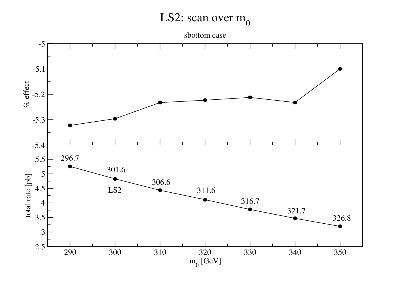
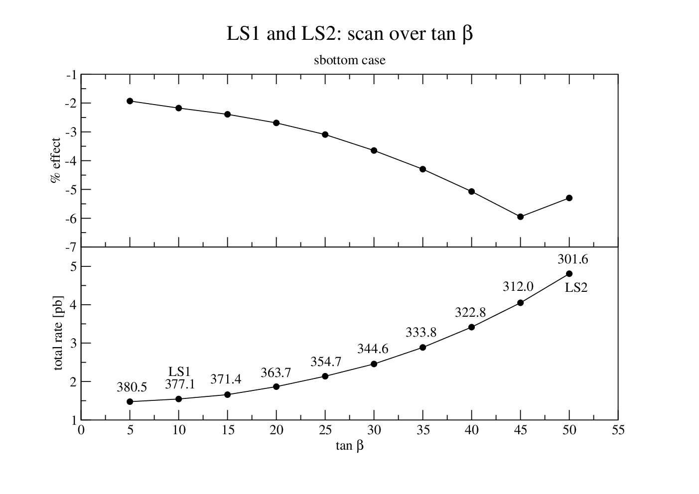
Our search of extra SUSY parameter dependence has been performed in the following way. For each benchmark point, we have varied in turn one of the four conventional parameters (, , and ) in a reasonable range, and computed the variable relative one loop effect and rate. For practical reasons we have only considered in the diagonal stop case the largely dominant component, and have shown the value of the mass which is generated by the variation of the chosen parameter. We anticipate, to shorten our presentation, that for diagonal stop production we shall only show in Figs. (13-18) the complete numerical results for those cases that seem to us reasonably meaningful, in particular that correspond to a total rate not below the 1 pb (extreme?) limit. This choice selects the set of LS1, LS2, SPS1a, SPS1a’, SPS1a slope and SPS5 benchmark points, but to perform a comparison with Ref.[3] we have also included the (perhaps academical) case of SPS2. For the remaining benchmark points, given the negligible value of their rates, we have only shown, for academic information, the dominant relative one loop effects in Fig.(19).
Figs.(13,14) show the results that we have obtained for the point SPS5, which is perhaps the most relevant one. As a general feature, common to all the considered cases, one sees that the SUSY one loop effects are almost systematically negative and small, of the few percent size. For what concerns the dependence on the chosen parameter, one sees for SPS5 that the variation of can produce a maximal variation of the relative effect of approximately three percent. A smaller variation, of approximately 1.5 percent, is generated in the considered range of . Varying and has essentially no practical effect ( below one percent) on the one loop contribution. The latter remains, in all cases, of the few percent at most.
In Figs.(15-18), to save space, we have only shown the maximal relative variation and the corresponding parameter. This choice selects for SPS1a, for SPS1a’, for SPS2, for LS1 and LS2. In the SPS1a’ case we have also plotted the dependence to perform a comparison with Ref.[3]. In all cases, the relative one loop effect is negative and small, typically of the one-two percent size.
A special case is that of the benchmark point SPS1a slope, where the parameters , and are related. In this case, we have plotted in Fig. (18) the variations with and . One sees that in the first case the relative negative effect can vary between one and four percent, remaining often in the three-four percent range. This represents the most relevant extra parameter dependence of our stop analysis. Varying can produce a smaller ( 1.5) effect, with an overall negative relative contribution in the five percent region which a priori might be visible with a dedicated experimental search.
An important step is now the comparison with previous results. Concerning the total rates, one can see from our curves that the values obtained for the points SPS1a, SPS1a’, SPS2 and SPS5 essentially reproduce, taking the corresponding stop mass values, the gluon-gluon component of Ref.[3] Table 1. For the parameter dependence, Ref.[3] shows the SPS1a’ case but uses, apart from , a different set of parameters. A comparison of the dependences for this point shows a qualitative agreement, i.e. a small and negative effect that increases with , although our values are slightly larger, in the three percent range. We conclude in this case, in full agreement with Ref.[3], that the dependence on the extra SUSY parameters is for SPS1a’ extremely small.
Another comparison can be performed for the SPS1a slope and SPS5 cases with the plots of Ref.[2]. Again one can see an essential agreement between our one-lop results and the Born results of Ref.[2], as one would expect given the smallness of our one loop effects.
The conclusion from our analysis of diagonal stop antistop production is that supersymmetric contributions due to extra SUSY parameters exist, but are generally apparently too small, at the few percent level, to produce an appreciable effect under realistic LHC experimental conditions, at least in a first luminosity phase. Our next step has been that of repeating our analysis for the diagonal sbottom-antisbottom production. Here we have only considered the LS1 and LS2 points, that would have a rate of the pb size. The results of our calculation are shown in the next Figures, that we now briefly comment.
As one sees from Figs.(20-23), the dependence of the effects on and is essentially negligible. For there is also no dependence on LS1, and a larger but irregular dependence (same values for different ) on LS2. The dependence on exhibits a different, and possibly appreciable, feature. One sees that the negative effect regularly increases with , like in the stop cases, but changing more, i.e. from 2 percent to 6 percent in the explored range. In particular, we believe that a relative effect of approximately six percent, in correspondence to a rate of the 5 pb size, might be, in principle, proposed for a highly dedicated experimental search.
In conclusion, a reasonable picture that seems to emerge from our combined analysis of the stop-antistop and sbottom-antisbottom diagonal production processes is that of a possible, although mild, dependence of the one-loop electroweak effect in the mSUGRA scenario on extra parameters. Keeping this result in mind, we have also computed, for all benchmark points, the non diagonal total rate derived from one-loop electroweak diagrams. We remind the reader that a calculation of the non diagonal rate, derived from annihilation at Born level via exchange, already exists [2] for SPS5. In the stop case, the value that is obtained is larger than that coming from the kinematically depressed NLO QCD diagrams, and is equal to pb. In the sbottom case, the value that is obtained is equal to pb. In Tabs. (3,4), we show the values that we have derived for the different benchmark points both for the one-loop diagrams and from the exchange calculations. One sees that the one-loop electroweak values are of the same size as those due to exchange and in some cases larger. This could have some relevance for the meaningful benchmark points. For example, in the LS2 stop production case, summing the one-loop with the -exchange contribution, one would get a total rate of approximately pb. This is a factor larger than the SPS5 point of [2], but realistically hard for experimental detection. A similar conclusion might be drawn for the rates of the remaining meaningful points if one sums the one-loop with the -exchange contributions. The results we have obtained for the sbottoms are similar, but because of the tiny cross sections involved, the experimental confirmation of our predictions will be again problematic.
V Conclusions
We have devoted our analysis to the search for extra (i.e. different from the final squark masses) parameters dependence in the processes of diagonal and non-diagonal stop-antistop and sbottom-antisbottom production from the initiated channel at EW NLO at LHC. With this aim, we have chosen twelve representative mSUGRA benchmark points and performed a variation of the mSUGRA parameters. We have verified in all cases the presence of a small (at the few percent level) relative difference of the effects with a more important role apparently played by different parameters for different points, in particular by in a case of sbottom production.
Certainly, the possibility of experimental verification of our conclusions would require very high luminosity scenarios and accuracies, representing a real challenge for the LHC experimental groups. This might, though, become interesting in case of a previous LHC supersymmetric production, which might justify the idea of the dedicated experimental effort that we have mentioned. In this respect, we should mention that the possibility of a determination of SUSY parameters dependence from the process of stop-chargino production has been already considered by us at Born level in a previous paper [16]. In view of the results obtained in this present search, we are now considering the derivation of the EW one-loop effects on stop-chargino production. The calculation is already in progress.
References
- [1] W. Beenakker, M. Kramer, T. Plehn, M. Spira and P. M. Zerwas, Stop production at hadron colliders, Nucl. Phys. B 515, 3 (1998) [arXiv:hep-ph/9710451].
- [2] G. Bozzi, B. Fuks and M. Klasen, Non-diagonal and mixed squark production at hadron colliders, Phys. Rev. D 72, 035016 (2005) [arXiv:hep-ph/0507073].
- [3] W. Hollik, M. Kollár and M. K. Trenkel, arXiv:0712.0287 [hep-ph].
- [4] T. Gehrmann, D. Maitre and D. Wyler, Nucl. Phys. B 703, 147 (2004) [arXiv:hep-ph/0406222].
- [5] G.J. Gounaris and F.M. Renard, Phys. Rev. Lett. 94,131601,2005, hep-ph/0501046; Addendum in Phys. Rev. D D73,097301,2006, hep-ph/0604041.
- [6] W.F.L. Hollik, Fortsch. Physik 38:165(1990).
- [7] T. Hahn and M. Perez-Victoria, Automatized one-loop calculations in four and D dimensions, Comput. Phys. Commun. 118, 153 (1999) [arXiv:hep-ph/9807565].
- [8] M. Beccaria, F.M. Renard and C. Verzegnassi, hep-ph/0203254; ”Logarithmic Fingerprints of Virtual Supersymmetry” Linear Collider note LC-TH-2002-005, GDR Supersymmetrie note GDR-S-081. M. Beccaria, M. Melles, F. M. Renard, S. Trimarchi, C. Verzegnassi, Int.Jour.Mod.Phys.A1850692003; hep-ph/0304110.
- [9] G. ’t Hooft and M. J. G. Veltman, Scalar One Loop Integrals, Nucl. Phys. B 153, 365 (1979).
- [10]
http://www.phys.psu.edu/
 cteq/
\bibitem{Beccaria:2004sx}
  M.
Beccaria, S. Bentvelsen, M. Cobal, F. M. Renard and C. Verzegnassi, Phys. Rev. D 71, 073003 (2005) [arXiv:hep-ph/0412249]. - [11] B. C. Allanach et al., The Snowmass points and slopes: Benchmarks for SUSY searches, in Proc. of the APS/DPF/DPB Summer Study on the Future of Particle Physics (Snowmass 2001) ed. N. Graf, In the Proceedings of APS / DPF / DPB Summer Study on the Future of Particle Physics (Snowmass 2001), Snowmass, Colorado, 30 Jun - 21 Jul 2001, pp P125 [arXiv:hep-ph/0202233].
- [12]
ATLAS Data Challenge 2 DC2 points:
http://paige.home.cern.ch/paige/fullsusy/romeindex.html. - [13] M. Beccaria, G. Macorini, F. M. Renard and C. Verzegnassi, Phys. Rev. D 74, 013008 (2006) [arXiv:hep-ph/0605108].
- [14] A. Djouadi, J. L. Kneur and G. Moultaka, Comput. Phys. Commun. 176 (2007) 426 [arXiv:hep-ph/0211331].
- [15] M. Frank, T. Hahn, S. Heinemeyer, W. Hollik, H. Rzehak and G. Weiglein, JHEP 0702 (2007) 047 [arXiv:hep-ph/0611326].
- [16] M. Beccaria, G. Macorini, L. Panizzi, F. M. Renard and C. Verzegnassi, Phys. Rev. D 74 (2006) 093009 [arXiv:hep-ph/0610075].
| mSUGRA scenario | |||||||||
|---|---|---|---|---|---|---|---|---|---|
| LS1 | 300 | 150 | -500 | 10 | + | 214.6 | 460.5 | 377.1 | 444.7 |
| LS2 | 300 | 150 | -500 | 50 | + | 224.7 | 430.4 | 301.6 | 399.3 |
| SPS1a | 100 | 250 | -100 | 10 | + | 399.7 | 585.5 | 515.7 | 546.6 |
| SPS1a’ | 70 | 250 | -300 | 10 | + | 367.3 | 581.9 | 504.4 | 541.7 |
| SPS1a slope | 0.4 | 250 | -0.4 | 10 | + | 399.7 | 585.5 | 515.7 | 546.6 |
| SPS2 | 1450 | 300 | 0 | 10 | + | 921.4 | 1289 | 1279 | 1540 |
| SPS3 | 90 | 400 | 0 | 10 | + | 645.2 | 840.3 | 790.1 | 823.7 |
| SPS4 | 400 | 300 | 0 | 50 | + | 540.1 | 692.5 | 614.9 | 687.2 |
| SPS5 | 150 | 300 | -1000 | 5 | + | 279.0 | 651.2 | 566.3 | 651.1 |
| SPS6 | 150 | 300 | 0 | 10 | + | 494.6 | 675.6 | 617.0 | 649.4 |
| SU1 | 70 | 350 | 0 | 10 | + | 566.4 | 754.0 | 698.6 | 729.8 |
| SU6 | 320 | 375 | 0 | 50 | + | 634.1 | 794.7 | 712.1 | 785.8 |
| LS1 | 27.00 @ | GeV | 1.54 @ | GeV |
|---|---|---|---|---|
| LS2 | 21.51 @ | GeV | 4.85 @ | GeV |
| SPS5 | 7.46 @ | GeV | 0.156 @ | GeV |
| SPS1a’ | 1.76 @ | GeV | 0.30 @ | GeV |
| SPS1a | 1.10 @ | GeV | 0.261 @ | GeV |
| SPS6 | 0.33 @ | GeV | 0.0908 @ | GeV |
| SPS4 | 0.19 @ | GeV | 0.090 @ | GeV |
| SU1 | 0.147 @ | GeV | 0.0416 @ | GeV |
| SU6 | 0.073 @ | GeV | 0.0358 @ | GeV |
| SPS3 | 0.066 @ | GeV | 0.0185 @ | GeV |
| SPS2 | 0.00617 @ | GeV | 0.00052 @ | GeV |
| LS2 | 0.0034 | 0.0058 |
| LS1 | 0.0026 | 0.0012 |
| SPS5 | 0.00057 | 0.00049 |
| SPS1a | 0.00054 | 0.00038 |
| SPS6 | 0.00022 | 0.00013 |
| SPS4 | 0.00017 | 0.00045 |
| SU1 | 0.00011 | 0.000057 |
| SU6 | 0.000080 | 0.00016 |
| SPS3 | 0.000057 | 0.000024 |
| SPS2 | 0.00000044 | 0.00000023 |
| LS2 | 0.0027 | 0.011 |
|---|---|---|
| LS1 | 0.00020 | 0.000024 |
| SPS5 | 0.000013 | 0.00000087 |
| SPS1a | 0.00020 | 0.000049 |
| SPS6 | 0.000068 | 0.0000067 |
| SPS4 | 0.00016 | 0.0006 |
| SU1 | 0.000040 | 0.0000032 |
| SU6 | 0.000081 | 0.00024 |
| SPS3 | 0.000017 | 0.0000012 |
| SPS2 |