Underground Muon Counters as a Tool for Composition Analyses
Abstract
The transition energy from galactic to extragalactic cosmic ray sources is still uncertain, but it should be associated either with the region of the spectrum known as the second knee or with the ankle. The baseline design of the Pierre Auger Observatory was optimized for the highest energies. The surface array is fully efficient above eV and, even if the hybrid mode can extend this range below eV, the second knee and a considerable portion of the wide ankle structure are left outside its operating range. Therefore, in order to encompass these spectral features and gain further insight into the cosmic ray composition variation along the transition region, enhancements to the surface and fluorescence components of the baseline design are being implemented that will lower the full efficiency regime of the Observatory down to eV. The surface enhancements consist of a graded infilled area of standard Auger water Cherenkov detectors deployed in two triangular grids of 433 m and 750 m of spacing. Each surface station inside this area will have an associated muon counter detector. The fluorescence enhancement, on the other hand, consists of three additional fluorescence telescopes with higher elevation angle () than the ones in operation at present. The aim of this paper is threefold. We study the effect of the segmentation of the muon counters and find an analytical expression to correct for the under counting due to muon pile-up. We also present a detailed method to reconstruct the muon lateral distribution function for the 750 m spacing array. Finally, we study the mass discrimination potential of a new parameter, the number of muons at 600 m from the shower axis, obtained by fitting the muon data with the above mentioned reconstruction method.
Keywords:
Cosmic Rays, Chemical Composition, Muon Detectors, , , , ,
1 Introduction
The cosmic rays energy spectrum extends for about eleven orders of magnitude, starting at energies below 1 GeV up to energies of more than eV. It presents three main features: the knee, the second knee and the ankle. There is evidence of a fourth feature, the so-called GZK suppression [1, 2], which is originated by the interaction of high energy protons with the photons of the cosmic microwave background. In the case of heavier nuclei, a similar effect is expected due to the fragmentation of the nuclei in their interaction with the photons of the microwave and infrared backgrounds [3].
The knee has been observed by several experiments [4, 5, 6] at around eV. At this energy the spectral index changes from to . The KASCADE data shows that the composition at the knee presents a transition from light to heavy primaries in such a way that, at energies above eV, the composition is dominated by heavy nuclei. These particles are originated in our Galaxy and what is being detected is, very likely, the end of the efficiency of supernova remnant shock waves as accelerators.
The second knee has been observed at around eV by Akeno [7], Fly’s Eye stereo [8], Yakutsk [9] and HiRes [10]. The physics of this feature is still unknown, it might be due to the end of the efficiency of supernova remnant shock waves as accelerators or a change in the diffusion regime in our Galaxy [11, 12].
The ankle is a broader feature that has been observed by Fly’s Eye [8] and Haverah Park [13], centered at approximately the same energy, eV. These results have been confirmed by Yakutsk [9], HiRes [10] and Auger in Hybrid mode [1]. AGASA also observed the ankle but at higher energy, around eV [14]. As in the case of the second knee, the origin of the ankle is still unknown and its physical interpretation is intimately related to the nature of the former. The ankle could be the transition between the Galactic and extragalactic components [15] or the result of pair creation by extragalactic protons in the interaction with the cosmic microwave background [16].
The precise determination of the mean chemical composition of the cosmic rays in the energy range above eV will allow us to understand the origin of the second knee and the ankle and to know the energy and the speed at which the transition between the Galactic and extragalactic components is given [17]. In particular, it will permit to decide among the three main models: (i) the mixed composition scenario [15], in which the composition injected by the extragalactic sources is assumed to be similar to the one of the Galactic sources and in which the transition takes place in the ankle region, (ii) the dip model [16], in which the ankle is originated by the interaction of extragalactic protons with the cosmic microwave background and the transition is given at the second knee and (iii) a two-component transition from Galactic iron nuclei to extragalactic protons, around the ankle energy [18].
The Pierre Auger Observatory consists of two Observatories situated one in each hemisphere. The Southern Observatory, located in Pampa Amarilla close to the city of Malargüe, Province of Mendoza, Argentina, currently consists of nearly 1600 Cherenkov detectors placed in a 1500 m triangular grid covering an area of 3000 km2 plus four fluorescence telescope buildings, with six telescopes each, situated in the periphery of the surface array and overlooking it. The construction started in 2000 and is going to be completed early in 2008. A complementary Northern Observatory will be sited in Colorado, United States of America.
The Southern Observatory, in its original design, is able to measure cosmic rays of energies above eV for the surface array and eV in hybrid mode. Two enhancements, AMIGA (Auger Muons and Infill for the Ground Array) [19] and HEAT (High Elevation Auger Telescopes) [20], will extend the energy range down to eV, encompassing the second knee and ankle region where the Galactic-extragalactic transition takes place.
AMIGA will consist of 85 pairs of Cherenkov detectors and 30 m2 muon counters buried m underground, placed in a graded infill of 433 m and 750 m triangular grids. The AMIGA infill area is bound by two hexagons covering areas of 5.9 km2 and 23.5 km2 corresponding to the 433 m and 750 m arrays, respectively. The energy thresholds of the 433 m and 750 m arrays are eV and eV, respectively [21]. On the other hand, HEAT will be formed by three additional telescopes of to elevation angle located next to the fluorescence telescopes building at Coihueco. They will be used in combination with the existing to elevation angle telescopes at Coihueco as well as in hybrid mode with the AMIGA infills.
These enhancements will also allow detailed composition studies based on the combined measurement of the atmospheric depth of maximum shower development, , and the shower muon content. These two parameters are very sensitive to primary mass composition. Other mass sensitive parameters, like the slope of the lateral distribution function, rise-time of the signals in the surface detectors, curvature radius, etc. strongly depend on them [22].
In this paper we will concentrate on the AMIGA muon detectors [19]. These counters will consist of highly segmented scintillators with optical fibers ending on 64-pixel multi-anode photomultiplier tubes (PMT). The scintillator strips will be equal to those used for the MINOS experiment [23]. The current baseline design calls for 400 cm long 4.1 cm wide 1.0 cm high strips of extruded polystyrene doped with fluors, POP () and POPOP (), and co-extruded with TiO2 reflecting coating. They are covered with reflective Al foil. To extract the scintillation light, a wavelength shifting fiber is glued into a grove which is machined along one face of the scintillator strip. A 10 m2 module will consist of 64 scintillator strips with the fibers ending on an optical connector matched to a 64-pixel multi-anode Hamamatsu H7546B PMT of 2 mm 2 mm pixel size, protected by a PVC casing. Each muon counter will consist of three of these 64-channel modules, totalling 192 independent channels covering an effective area of 30 m2 (actually during the engineering array phase one of these 10 m2 modules from each counter will be split into two 5 m2 modules for further analyses close to the shower core). These muon counters will be buried alongside a water Cherenkov tank. Each of the 192 channels of the electronics will count pulses above a given threshold, with an overall counter time resolution of 20 ns.
We also present a detailed method for the reconstruction of the Muon Lateral Distribution Function (MLDF) from data obtained by the muon counters of the 750 m-array. An associated problem is the pile-up effect due to the finite segmentation of the muon counters. We analyse this problem and propose a correction that considerably improves the reconstruction of the MLDF. The number of muons at 600 m from the shower axis, , is extracted from MLDF fits using our reconstruction method. Subsequently, the design parameters of the muon counters (segmentation and area) are validated by studying the impact of these parameters on the total uncertainty. Finally, we study the mass discrimination power of as compared to other parameters normally used in composition analyses: the maximum development of the longitudinal profile, , the curvature radius of the shower front, , rise time of the signal at the water Cherenkov detectors, , and slope of the lateral distribution function of the total signal deposited in the water Cherenkov detectors, . Second order effects, like multiple triggering due to electrons scattered by a single muon, will be dealt with in a subsequent work.
2 Muon Counter Segmentation
The AMIGA counter electronics just counts pulses above a given threshold, without a detailed study of signal structure or peak intensity. This method is very sturdy since it does not rely on deconvoluting the number of muons from an integrated signal. It does not depend on the PMT gain or gain fluctuations nor on the muon hitting position on the scintillator strip and the corresponding light attenuation along the fiber track. Neither does it require thick scintillators to control Poisson fluctuations in the number of photo electrons per impinging muon. But this one-bit electronics design relies on a fine counter segmentation to prevent undercounting due to simultaneous muon arrivals.
2.1 Characteristic distance to the nearest station
The optimum segmentation of the muon counters depends on the number of muons arriving in the time given by the system time resolution. Since the MLDF decreases very rapidly with the distance to the shower axis we need to determine the average position of the closest station, where pile-up is more significant.
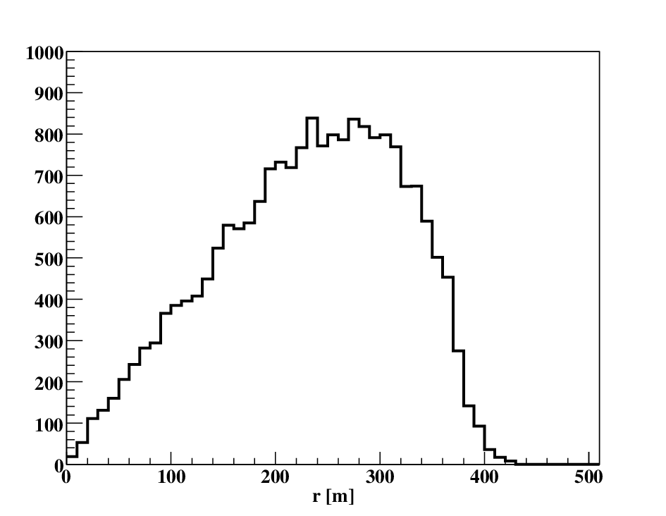
The position of the first station depends on the geometry of the array and the angular distribution of cosmic rays. We performed a simple Monte Carlo calculation for the m-array. We uniformly distributed impact points in a triangular grid with arrival directions following a distribution with zenith angle and a uniform distribution for the azimuth angle . For each event we obtained the distance (along the shower plane) between the shower core and the closest station. Figure 1 shows the obtained distribution, with a mean value at m. Therefore, we will base our subsequent studies on the number of muons found at a characteristic distance of 200 m.
2.2 Underground muons at the nearest station
To prevent contamination due to charged electromagnetic particles of the shower, the muon counters will be buried underground. Muons lose energy mainly by ionization when they propagate through the soil. Assuming that the energy loss is proportional to the track length, the energy of a muon that travelled a distance is given by,
| (1) |
where is the initial energy of the muon, we assume a soil density of g cm-3 and MeV cm2 g-1 is the fractional energy loss per depth of standard rock ( and ) [24].
Showers initiated by iron nuclei produce more muons than those from lighter nuclei of the same energy. For that reason the simulations were performed with iron showers to take into account the most unfavorable case. We assumed 20 ns of sampling time for the system time resolution.
Figure 2 shows the time distribution of muons in bins of ns at 200 m from the shower core, in an area of 30 m2 (muon counter area projected on the shower plane) and at 2.5 m depth for simulated iron showers of , primary energy eV and using QGSJET-II [29, 30] as the high energy hadronic interaction model. We used Aires version 2.8.2 [31] to simulate air showers and, to obtain the muon time distribution, we propagated them through the soil assuming that they move at the speed of light and the energy loss is given by Eq. (1). Note that only muons with ( zenith angle of the individual muons) reach the detector.
From figure 2 we can see that the maximum number of muons at eV and in the first 20 ns-bin is about .

2.3 Muon pile-up correction
The probability distribution corresponding to a given number of muons that hit a segmented detector in a time interval is multinomial,
| (2) |
where is the number of segments, is the total number of muons and is the number of muons that hit the th segment, i. e. .
As the AMIGA muon counter electronics will be designed to only count events above a certain threshold, without analysing the corresponding signal, whenever two or more muons hit the same scintillator strip in the same time bin, these multiple muons will be counted as one. Therefore, the total number of muons counted is given by,
| (3) |
where if and if .
By using Eq. (2) we can calculate the mean value and the variance of ,
| (4) | |||||
| (5) | |||||
Figure 3 shows the number of counted muons as a function of the incident muons for a muon counter with 192 segments.

To correct the effect of segmentation we can invert Eq. (4),
| (6) |
The number of muons inferred, , obtained from Eq. (6) has an error which can be estimated by solving for a given the following equations,
| (7) | |||||
| (8) |
where and , the unknowns, are the upper and lower limits of the error interval, respectively. The error associated with is asymmetric, this is due to the shape of as a function of . If we define and , we can see that and that the difference increases with .
To assess the importance of the error introduced with the use of the correction formula, it has to be compared to the Poissonian fluctuations inherent to the process of counting the muons that hit each scintillator strip in a given time bin. Therefore, the total error in the determination of the number of muons is , where is the error corresponding to the Poissonian fluctuations.
Figure 4 shows the ratio between the total error and the Poissonian one as a function of the number of muons obtained after correction for 192 segments. From this figure we see that for 90 incident muons the total error is greater than the Poissonian by less than , and as such there is no need to further segment the detector. Note that the individual uncertainty in each muon counter will not directly translate to the but that it will be further reduced when a number of counters are used to fit the MLDF.
It is worth emphasizing that AMIGA envisages an experimental verification of the segmentation, since in its unitary cell with 7 counters, the modules will have double segmentation.

3 Reconstruction of the MLDF
One of the first MLDF parametrizations was introduced by K. Greisen [25],
| (9) |
where is the distance to the shower axis, m and is a normalization constant that depends on the atmospheric depth . Subsequently other groups proposed different functional forms [26, 27]. Although all these formula describe the MLDF very accurately in the range of short and intermediate distances, they are not so good at larger distances and for higher-energy showers. Recently the KASCADE-Grande Collaboration proposed a new MLDF parametrization which is a modification of the Greisen formula [28],
| (10) |
where , , , and are parameters which define the shape and size of the MLDF.
To study the shape of the underground MLDF we performed air shower simulations. Again, we used Aires 2.8.2 with QGSJET-II and to propagate the muons in the soil we used Eq. (1). Figure 5 shows the simulated MLDFs at 2.5 m underground corresponding to showers initiated by protons and iron nuclei of of zenith angle and for several primary energies. It also shows the fits of the profiles with the KASCADE-Grande MLDF where we fixed the parameters m and and left , and as free fit parameters. The simulated profiles are fitted very accurately in the range of distances considered.

The range of primary energies for which we simulated MLDFs in order to fit them with the KASCADE-Grande formula was eV - eV in steps of . This procedure was performed for both protons and iron nuclei at and .
The parameter in Eq. (10) describes the behavior of the MLDF at relatively large distances from the core, where only low statistics are available in general. On the other hand, is well sampled by the proposed 750 m-array.
Therefore, for all practical purposes, the analysis shows that a better fit of the muon counters data to the complete MLDF function is obtained by just fixing , its average value for protons, while leaving and as free parameters. The factor involving only becomes important at distances to the shower core larger than km, well beyond the point where data is available at the energies of interest. To keep free when dealing with real data would only add degrees of freedom to the fitting function without the corresponding increase in the available data.
To develop the reconstruction method it is necessary to simulate an array of Cherenkov detectors with associated muon counters. The Cherenkov detectors give the trigger information, geometry and energy reconstructions, synchronization, and telecommunications. For this purpose we interfaced an ad-hoc developed muon counter computer code with the program SDSim version v3r0 [32], which simulates the Pierre Auger surface detectors.
Since the number of particles produced in a shower is extremely large, in a eV shower, it is practically impossible to follow and store all the information of the secondary particles. Therefore, a statistical method called thinning, first introduced by M. Hillas [33, 34], is used. An unthinning method has to be applied to calculate the real number of muons arriving at a counter. We employed the method introduced by P. Billoir described in references [35, 36].
The muons with enough energy to reach the detector that arrive in a time interval are uniformly distributed and those that fall into the same segment are counted as one, in this way we include in the simulation the pile-up effect introduced by the electronics. The present simulation does not include the propagation of the electromagnetic particles into the soil. Detailed numerical simulations involving Geant4 [37] and Aires show that, beyond radiation lengths, the electromagnetic contribution is at most a few percent [38] and can therefore be neglected in the present analysis. Nevertheless, these punch through simulations will be experimentally verified by a specific detector [39].
We used the generated showers to study the shape of the MLDF to simulate the response of the Cherenkov detectors and muon counters by randomly distributing impact points in the 750 m-array. We used muon counters of m2, 192 segments and a time resolution of ns. For each muon counter we calculated the “real” muon distribution (i.e., assuming an infinite segmentation, without pile-up effect), the “measured” muon distribution (taking into account the pile-up effect) and the corrected muon distribution (obtained applying Eq. (6) in each time bin).
As an example, figure 6 shows the “measured” time distribution of muons in a muon detector at 227 m from the shower core for a simulated event initiated by an iron primary of eV and . Figure 6 also shows the “real” time distribution and the corrected one.

In this example, the total number of muons corresponding to the real distribution is and the measured one is , less approximately. The total number of muons after applying the correction is , about less than the real value. This shows the importance of the correction in the determination of the number of muons at each counter, especially at those close to the shower core.
Due to the pile-up effect, counters are not able to measure the number of muons very close to the shower axis. Therefore and to avoid systematic uncertainties it is convenient to fit the MLDFs including stations with a large number of muons in a different way. We will consider as saturated stations those with (i.e. ) in at least one time bin.
The probability of having more than 3 background triggers due to random coincidences in a time window is, , where , is the vertical intensity of the background and is the muon counters area. The background flux at m underground in the site where the muon counters are going to be installed is under study. However, if we assume a vertical intensity like the corresponding to the Auger tanks (see Ref. [40]) we obtain and for a vertical intensity 10 times larger, which can be considered as an upper limit, . Therefore, stations with 0, 1 or 2 muons will be considered as silent stations to prevent errors coming from such random coincidences. We will take into account all silent stations with distance to the shower core less than m.
The number of muons that hit a given detector follows a Poisson distribution. Therefore, to fit the MLDF we minimize the likelihood function with respect to the parameters of the KASCADE-Grande MLDF (see Eq. (10)), where
| (11) | |||||
Here the first factor corresponds to saturated stations, the second to “good” stations (neither saturated nor silent) and the third to silent ones. is the distance of the -th station to the shower core, is the number of saturated stations, is the number of “good” stations, is the number of silent stations, is the total number of muons measured corresponding to the -th station and is the total number of muons for the -th station after applying the correction in every time bin of the measured time distribution.
The expression for the saturated stations comes from the fact that the Poisson distribution of mean value can be approximated by a Gaussian distribution of mean value and , . Therefore, the probability that be greater than a given is,
| (12) |
where,
| (13) |
The expression for the silent stations corresponds to the probability that the number of muons be less or equal than two,
| (14) |
Figure 7 shows a fit of the MLDF for the same event of figure 6. To reconstruct the arrival direction and the position of the shower core we used the standard package, called CDAS [41], used to reconstruct the information from the Auger Cherenkov detectors. The arrows correspond to the positions of the silent stations.

In order to stress the importance of including the silent and saturated stations in the fit procedure, figure 8 shows the fits corresponding to proton events of eV and , with (solid line) and without (dashed line) taking into account the silent and saturated stations. We observe that the fitted MLDF is much more similar, specially close to 600 m from the shower axis, to the real one (histogram of the figure) for the case in which the silent and saturated stations are included in the fit. The exclusion of the silent and saturated stations produces a spurious flattening of the fitted MLDF, specially for those cases in which the closest station is saturated, as clearly shown in bottom panel of figure 8. The discrepancies between the fitted MLDF obtained without including the silent and saturated stations and the real one increases for decreasing primary energies. It introduces important biases in particular in the distribution. The inclusion of the saturated and silent stations avoid these biases and reduce the error in the determination of .


4 Muons at 600 m from the Shower Core
The number of muons at a given distance from the shower axis has been used in the past as a parameter for composition analysis. The AMIGA 750 m infill has a detector spacing appropriate to evaluate the number of muons at m from the shower core [42].
The discrimination power of depends strongly on its reconstruction uncertainty. Therefore, to study the uncertainty introduced by the reconstruction method we define,
| (15) |
where is the reconstructed number of muons from a MLDF fit and is the expected average number of muons from sampling muons in a 40 m wide ring (in the shower plane), both at 600 m from the shower axis.
Figure 9 shows (relative error of ), obtained from Gaussian fits of the distributions of , as a function of the logarithm of the energy for proton and iron primaries and zenith angles of and . We considered muon counters of m2, 192 segments and a time resolution of 20 ns (solid lines). As expected, the relative error decreases with energy, due to the fact that the number of muons in the showers increases almost linearly with primary energy, therefore, the number of triggered muon detectors (with ) also increases.


From figure 9 we can also see that the relative error for the iron nuclei is smaller than the corresponding one for protons because heavier nuclei produce more muons.
To study the robustness of the reconstruction method we assumed a time binning much larger than the width of the time distribution of muons, the worst case. Figure 9 shows the obtained results (dashed lines), the relative error does not increase much, with respect to the case of 20 ns.
Note that for the two cases considered the mean value of , i. e. the bias in the determination of , kept less than in the whole energy range considered (from eV to eV).
The uncertainty of is less than in the energy range in which the 750 m-array will be effective, from eV to eV. Moreover, it decreases with energy, such that for energies greater than eV it is smaller than . The error in the reconstruction of the primary energy is typically around [43], and because the number of muons increases almost linearly with the energy this uncertainty will dominate in the determination of . Therefore, muon counters of 30 m2 and 192 segments are acceptable values for the design parameters.
5 Parameters Sensitive to the Chemical Composition
Several parameters obtained from the surface and fluorescence detectors are used for the identification of the primary. The difference between parameters corresponding to different primaries is due to the fact that showers initiated by heavier primaries develop earlier and faster in the atmosphere and also have a larger muon content.
From the distributions of corresponding to a given energy, type of primary and zenith angle, we calculated the mean value and the regions of and of probability. Figure 10 shows and the regions of and probability (parameter P in the figure) as a function of the energy for protons and iron nuclei of 30∘ of zenith angle. Although the distributions for iron and proton show an overlap, the separation is good at confidence level.

Besides the muon content of the shower and the depth of the maximum there are other parameters that are used for composition analysis [44]. These are the structure of the shower front (in particular the rise-time of the signals in the surface detectors), the radius of curvature, , and the slope, , of the lateral distribution function of the total signal deposited in the water Cherenkov detectors.
For any given event, we can define a parameter related to the shower front structure, using the rise-time of the signals in a selected subset of the triggered water Cherenkov detectors,
| (16) |
where is the number of stations with signal greater than VEM 11 1 Vertical Equivalent Muon, signal deposited in a water Cherenkov tank when fully traversed by a muon vertically impinging in the center of the tank [40], and are the times at which and of the total signal is collected, respectively, and is the distance of the -th station to the shower axis. Only stations at a distance to the shower axis greater than m are included in Eq. (16).
To obtain , including the effect of the detectors and the reconstruction procedure, we assumed that the distribution of the reconstructed is a Gaussian with an energy dependent as given in Ref. [20]. Therefore, we obtained the distributions of the reconstructed from the simulated showers by sampling a value from a Gaussian distribution with the mean value given by calculated internally in Aires and from the interpolation of the simulated data of Ref. [20].
To compare the discrimination power of the different parameters considered () we define,
| (17) |
where is the parameter for the nucleus , is the mean value and the standard deviation for the distribution of . From the definition of we see that the larger its value, the greater the discrimination power of the parameter .
Presumably, the interpolated signal of the water Cherenkov detectors at 600 m from the shower axis will be used to obtain the primary energy for the 750 m-array. Therefore, to study its dependence on the primary mass we included it in the set of parameters. Figure 11 shows the linear fits of as a function of the logarithm of the energy for and and for the different parameters considered.


From figure 11 we see that the parameter which better separates protons from iron nuclei appears to be , followed by . We can also see that, except for , increases with the primary energy. This happens because, as the energy increases, the number of triggered stations also increases, which reduces the reconstruction errors. The number of particles in the detectors also increases with the energy and therefore reduces fluctuations.
Although the reconstruction error of decreases with primary energy, slowly decreases. This happens because the mean values of corresponding to protons and iron nuclei get closer as the energy increases for the hadronic model considered (however, this is not the case for the hadronic model EPOS, see Ref. [45]).
If the energy uncertainty is negligible, is the best parameter for mass discrimination analysis. However, as opposed to the other parameters which depend on the energy logarithmically, the number of muons is almost proportional to the primary energy. Therefore, the energy uncertainty will affect more the discrimination power of than that of the other parameters. Figure 12 shows as a function of the energy assuming a energy uncertainty for the parameters and (see appendix A for the details of the calculation). We see that the discrimination power of decreases in such a way that it is of the order of the corresponding to . From figure 12 we also see that the discrimination power of remains approximately the same when the energy uncertainty is included, which is due to its logarithmic dependence on the primary energy.


6 Conclusions
In this paper we studied the effect of muon counter segmentation and we found an analytical expression to correct for the undercounting due to muon pile-up. We presented a detailed method to reconstruct the muon lateral distribution function for the 750 m infill array. We also studied the potential of the parameter as a discriminator of the identity of the primary cosmic ray particle.
We showed that for 192 segments and 90 incident muons in a 20 ns time bin (maximum number of muons at 200 m from the shower axis for eV, which would correspond to saturation for the adopted configuration) the total error, Poissonian plus pile-up correction, does not exceed the Poissonian error by more than . This correction is enough to attain, with surface information alone, a composition discrimination power comparable, or even better, than that of . Clearly, this result depends quantitatively on the assumed hadronic interaction model and, consequently, the safest conclusion is probably that a two-dimensional analysis, including both parameters, might well configure an optimal composition analysis method which will be discussed in an accompanying paper [46].
The error in the determination of parameter is at eV (energy threshold of the 750 m array) and decreases as the energy increases, being less than for eV. So, at this energy or greater, this uncertainty is small compared with the expected primary energy uncertainty, , which affects directly the determination of since shower muon content is nearly proportional to the primary energy. Therefore, m2 individual muon detectors partitioned in 192 segments, can be considered as an optimal compromise between cost and scientific output.
We also studied the effect of the energy uncertainty on the discrimination power of . The inclusion of this effect somewhat degrades the discrimination power of , however, it generally remains as good a parameter as .
7 Acknowledgments
The authors have greatly benefited from discussions with several colleagues from the Pierre Auger Collaboration, of which they are members. We also want to acknowledge Corbin Covault for carefully reading the manuscript and for his valuable comments. GMT acknowledges the support of DGAPA-UNAM through grant IN115707.
Appendix A Effect of the Energy Uncertainty
We estimate the effect of the energy uncertainty on the discrimination power of the parameters and , assuming a power law spectrum of spectral index , , and a gaussian uncertainty in the energy determination of with the relative error. Let be a parameter for which we know its distribution function parametrized by the primary energy, . Therefore, the conditional probability of given the reconstructed energy is,
| (18) |
where eV and eV are the lower and upper limits of the part of the spectrum considered, respectively, and,
| (19) |
From Eq. (18) we can calculate the mean value and the variance of the parameter as a function of the reconstructed energy,
| (20) | |||||
| (21) | |||||
where and are the mean value and the variance of parameter without taking into account the energy uncertainty, calculated using . Therefore, to calculate the parameter defined in Eq. (17) including the energy uncertainty, we need the functions and for each parameter considered. For that purpose, we fitted the mean value and the standard deviation of with a function of the form and for with . Using the fits obtained for and and Eqs. (20), (21) and (17) we obtain which can be seen in Figure 12 for .
References
- [1] Y. Tokonatsu for the Pierre Auger Collaboration, Proc. 30th ICRC (Mérida-México), 318 (2007).
- [2] D. Bergman for the HiRes Collaboration, Proc. 30th ICRC (Mérida-México), 1128 (2007).
- [3] D. Allard, E. Parizot, E. Khan, S. Goriely and A. V. Olinto, Astron. Astrophys. 443, L29 (2005).
- [4] K. H. Kampert et al. (KASCADE Coll.), arXiv:astro-ph/0405608.
- [5] M. Aglietta et al. (EAS-TOP and MACRO Coll.), Astropart. Phys. 20, 641 (2004).
- [6] T. Antoni et al., Astropart. Phys. 24, 1 (2005).
- [7] M. Nagano et al., J. Phys. G 10, 1295 (1984).
- [8] T. Abu-Zayyad et al., Astrphys. J. 557, 686 (2001).
- [9] M. I. Pravdin et al., Proc. 28th ICRC (Tuskuba) 389 (2003).
- [10] HiRes Collaboration, Phys. Rev. Lett. 92, 151101 (2004).
- [11] J.R. Hoerandel, Astropart. Phys. 19, 193 (2003).
- [12] J. Candia et al., JHEP 0212, 033 (2002).
- [13] M. Ave et al., Proc. 27th ICRC (Hamburg) 381 (2001).
- [14] M. Takeda et al., Astropart. Phys. 19, 447 (2003).
- [15] D. Allard, E. Parizot and A. V. Olinto, Astropart. Phys. 27, 61 (2007).
- [16] V. Berezinsky, S. Grigor’eva and B. Hnatyk, Astropart. Phys. 21, 617 (2004).
- [17] G. Medina-Tanco for the Pierre Auger Collaboration, Proc. 30th ICRC (Mérida-México), 991 (2007).
- [18] T. Wibig and A. Wolfendale, J. Phys. G31, 255 (2005).
- [19] A. Etchegoyen for the Pierre Auger Collaboration, Proc. 30th ICRC (Mérida-México), 1307 (2007).
- [20] H. Klages for the Pierre Auger Collaboration, Proc. 30th ICRC (Mérida-México), 65 (2007).
- [21] M. C. Medina et al., Nucl. Inst. and Meth. A566, 302 (2006).
- [22] A. Chou et al., Proc. 26th ICRC 7, 319 (2005).
- [23] The MINOS detectors Technical Design Report, Version 1.0, October 1998.
- [24] W. M. Yao et al., J. Phys. G33, 1 (2006).
- [25] K. Greisen, Ann. Rev. Nucl. Sci. 10, 63 (1960).
- [26] M. Hillas et al., Acta Phys. Acad. Sci. Hung. 29 Suppl. 3, 533 (1970).
- [27] R. Brownlee et al., Acta Phys. Acad. Sci. Hung. 29 Suppl. 3, 651 (1970).
- [28] J. Buren, T. Antoni, W. Apel, et al., Proc. 26th ICRC 6, 301 (2005).
- [29] S. Ostapchenko, arXiv:astro-ph/0412591 (2004).
- [30] S. Ostapchenko, arXiv:hep-ph/0501093 (2005).
- [31] S. Sciutto, AIRES user’s Manual and Reference Guide (2002), http://www.fisica.unlp.edu.ar/auger/aires.
- [32] http://lpnhe-auger.in2p3.fr/Sylvie/WWW/AUGER/DPA.
- [33] A. Hillas, Proc. 19th ICRC 1, 155 (1985).
- [34] A. Hillas, Nucl. Phys. (Proc. Suppl.) B52, 29 (1997).
- [35] M. Risse et al., Proc. 27th ICRC (Hamburg-Germany), 552 (2001).
- [36] A. D. Supanitsky, PhD thesis of the University of Buenos Aires.
- [37] http://geant4.web.cern.ch/geant4/
- [38] F. Sanchez et al., Proc. 30th ICRC (Mérida-México), 1276 (2007).
- [39] F. Sanchez et al., Proc. 30th ICRC (Mérida-México), 1277 (2007).
- [40] X. Bertou et al., Nucl. Instr. and Meth. A568, 839 (2006).
- [41] http://www.auger.org.ar/CDAS-Public.
- [42] N. Hayashida et al., J. Phys. G: Nucl. Part. Phys. 21, 1101 (1995).
- [43] M. Roth for the Pierre Auger Collaboration, Proc. 30th ICRC (Mérida-México), 313 (2007).
- [44] D. Supanitsky et. al., Proc. 29th ICRC 7, 37 (2005).
- [45] M. Unger for the Pierre Auger Collaboration, Proc. 30th ICRC (Mérida-México), 594 (2007).
- [46] D. Supanitsky et al., to be submitted to Astropart. Phys.