Composing Quantum Protocols in a Classical Environment
Abstract
We propose a general security definition for cryptographic quantum
protocols that implement classical non-reactive two-party tasks. The
definition is expressed in terms of simple
quantum-information-theoretic conditions which must be satisfied by
the protocol to be secure. The conditions are uniquely determined by
the ideal functionality defining the cryptographic task to be
implemented. We then show the following composition result. If
quantum protocols securely implement ideal
functionalities according to our security
definition, then any purely classical two-party protocol,
which makes sequential calls to , is equally
secure as the protocol obtained by replacing the calls to
with the respective quantum protocols
. Hence, our approach yields the minimal
security requirements which are strong enough for the typical use of
quantum protocols as subroutines within larger classical
schemes. Finally, we show that recently proposed quantum protocols
for oblivious transfer and secure identification in the
bounded-quantum-storage model satisfy our security definition, and
thus compose in the above sense.
Keywords: two-party quantum cryptography, composability, identification, oblivious transfer
1 Introduction
Background.
Finding the right security definition for a cryptographic task is a non-trivial fundamental question in cryptography. From a theoretical point of view, one would like definitions to be as strong as possible in order to obtain strong composability guarantees. However, this often leads to impossibility results or to very complex and inefficient schemes. Therefore, from a practical point of view, one may also consider milder security definitions which allow for efficient schemes, but still offer “good enough” security.
It is fair to say that in computational cryptography, the question of defining security and the trade-offs that come along with these definitions are by now quite well understood. The situation is different in quantum cryptography. For instance, it was realized only recently that the standard security definition of quantum key-agreement does not guarantee the desired kind of security and some work was required to establish the right security definition [GL03, RK05, BHL+05, Ren05, KRBM07]. In [BM04, Unr04], strong security definitions for general quantum protocols were proposed by translating Canetti’s universal-composability framework and Backes, Pfitzmann and Waidner’s reactive-simulatability model, respectively, into the quantum setting. The resulting security definitions are very strong and guarantee full composability. However, they are complex and hard to achieve. Indeed, so far they have been actually used and shown to be achievable only in a couple of isolated cases: quantum key distribution [BHL+05] and quantum multi-party computation with dishonest minority [BCG+05]. It is still common practice in quantum cryptography that every paper proposes its own security definition of a certain task and proves security with respect to the proposed definition. However, it usually remains unclear whether these definitions are strong enough to guarantee any kind of composability, and thus whether protocols that meet the definition really behave as expected.
Contribution.
We propose a general security definition for quantum protocols that implement cryptographic two-party tasks. The definition is in terms of simple quantum-information-theoretic security conditions that must be satisfied for the protocol to be secure. In particular, the definition does not involve additional entities like a “simulator” or an “environment”. The security conditions are uniquely determined by the ideal functionality that defines the cryptographic task to be realized. Our definition applies to any non-reactive, classical ideal functionality , which obtains classical (in the sense of non-quantum) input from the two parties, processes the provided input according to its specification, and outputs the resulting classical result to the parties. A typical example for such a functionality/task is oblivious transfer (OT). Reactive functionalities, i.e. functionalities that have several phases (like e.g. bit commitment), or functionalities that take quantum input and/or produce quantum output are not the scope of this paper.
We show the following composition result. If quantum protocols securely implement ideal functionalities according to our security definition, then any purely classical two-party protocol, which makes sequential calls to , is equally secure as the protocol obtained by replacing the calls to with the respective quantum subroutines . We stress that our composition theorem, respectively our security definition, only allows for the composition of quantum sub-protocols into a classical outer protocol. This is a trade-off which allows for milder security definitions (which in turn allows for simpler and more efficient implementations) but still offers security in realistic situations. Indeed, current technology is far from being able to execute quantum algorithms or protocols which involve complicated quantum operations and/or need to keep a quantum state ‘‘alive’’ for more than a tiny fraction of a second. Thus, the best one can hope for in the near future in terms of practical quantum algorithms is that certain small subroutines, like key-distribution or OT, may be implemented by quantum protocols, while the more complex outer protocol remains classical. From a more theoretical point of view, our general security definition expresses what security properties a quantum protocol must satisfy in order to be able to instantiate a basic cryptographic primitive upon which an information-theoretic cryptographic construction is based. For instance, it expresses the security properties a quantum OT11 1 We are well aware that quantum OT is impossible without any restriction on the adversary, but it becomes possible for instance when restricting the adversary’s quantum memory [DFSS05, DFR+07]. needs to satisfy so that Kilian’s classical22 2 Here, “classical” can be understood as “non-quantum” as well as “being a classic”. construction of general secure function evaluation based on OT [Kil88] remains secure when instantiating the OT primitive by a quantum protocol. Alternatively, our security conditions can also be viewed as providing the minimal requirements for a quantum protocol to behave as expected.
Finally, we show that the ad-hoc security definitions proposed by Damgård, Fehr, Salvail and Schaffner for their 1-2 OT and secure-identification protocols in the bounded-quantum-storage model [DFR+07, DFSS07] imply (and are likely to be equivalent) to the corresponding security definitions obtained from our approach.33 3 Interestingly, this is not true for the definition of Rabin OT given in the first paper in this line of research [DFSS05], and indeed in the full version of that paper, it is mentioned that their definition poses some “composability problems” (this problem though has been fixed in the journal version [DFSS08]). This supports our claim that failure of satisfying our security definition is strong evidence for a security problem of a quantum protocol. This implies composability in the above sense for these quantum protocols in the bounded-quantum-storage model.
Related work.
In the classical setting, Crépeau, Savvides, Schaffner and Wullschleger proposed information-theoretic conditions for two-party secure function evaluation [CSSW06], though restricted to the perfect case, where the protocol is not allowed to make any error. They show equivalence to a simulation-based definition that corresponds to the standard framework of Goldreich [Gol04]. Similar conditions have been subsequently found by Crépeau and Wullschleger for the case of non-perfect classical protocols [CW08]. Our work can be seen as an extension of [CSSW06, CW08] to the setting where classical subroutines are implemented by quantum protocols.
As pointed out and discussed above, general frameworks for universal composability in the quantum setting have been established in [BM04, Unr04]. The composability of protocols in the bounded-quantum-storage model has recently been investigated by Wehner and Wullschleger [WW08]. They propose security definitions that guarantee sequential composability of quantum protocols within quantum protocols. This is clearly a stronger composition result than we obtain (though restricted to the bounded-quantum-storage model) but comes at the price of a more demanding security definition. And indeed, whereas we show that the simple definitions used in [DFSS05, DFR+07] already guarantee composability into classical protocols without any modifications to the original parameters and proofs, [WW08] need to strengthen the quantum-memory bound (and re-do the security proof) in order to show that the 1-2 OT protocol from [DFR+07] meets their strong security definition. As we argued above, this is an overkill in many situations.
2 Notation
Quantum States. We assume the reader’s familiarity with basic notation and concepts of quantum information processing [NC00].
Given a bipartite quantum state , we say that is classical if is of the form for a probability distribution over a finite set . This can be understood in that the state of the quantum register depends on the classical random variable , in the sense that is in state exactly if . For any event defined by for all , we may then write
| (1) |
When we omit registers, we mean the partial trace over these register, for instance , which describes given that the event occurs.
This notation extends naturally to states that depend on several classical random variables , etc., defining the density matrices , , etc. We tend to slightly abuse notation and write and , as well as and . Given a state with classical , by saying that “there exists a classical random variable such that satisfies some condition”, we mean that can be understood as for some state with classical and , and that satisfies the required condition.44 4 This is similar to the case of distributions of classical random variables where given the existence of a certain is understood that there exists a certain joint distribution with .
is independent of (in that does not depend on ) if and only if , which in particular implies that no information on can be learned by observing only . Similarly, is random and independent of if and only if , where is the density matrix of the fully mixed state of suitable dimension.
We also need to express that a random variable is independent of a quantum state when given a random variable . This means that when given , the state gives no additional information on . Yet another way to understand this is that is obtained from and by solely processing . Formally, adopting the notion introduced in [DFSS07], this is expressed by requiring that equals , where the latter is defined as
In other words, precisely if for all and . This notation naturally extends to .
Full (conditional) independence is often too strong a requirement, and it usually suffices to be “close” to such a situation. Closeness of two states and is measured in terms of their trace distance , where for any operator , is defined as . We write to denote that , and we then say that and are -close. It is known that -closeness is preserved under any quantum operation; this in particular implies that if then no observer can distinguish from with advantage greater than [RK05]. For states and with classical and , it is not hard to see that , and thus if . In case of purely classical states and , the trace distance coincides with the statistical distance of the random variables and : , and we then write , or , instead of .
We will make use of the following lemmas whose proofs are given in Appendix 0.A.
Lemma 1
- 1.
If then .
- 2.
If then .
- 3.
If , then .
Lemma 2
If then for any function .
Lemma 3
For an event which is completely determined by the random variable , i.e. for all , the probability either vanishes or equals one, we can decompose the density matrix into55 5 One is tempted to think that such a decomposition holds for any event ; however, this is not true. See Lemma 2.1 of [DFSS07] for another special case where the decomposition does hold.
3 Protocols and Functionalities
Quantum Protocols.
We consider two-party quantum protocols , consisting of interactive quantum algorithms and . For convenience, we call the two parties who run and Alice and Bob, respectively. There are different approaches to formally define interactive quantum algorithms and thus quantum two-party protocols, in particular when we restrict in- and outputs (of honest participants) to be classical. For instance such a formalization can be done by means of quantum circuits, or by means of a classical Turing machine which outputs unitaries that are applied to a quantum register. For our work, the specific choice of the formalization is immaterial; what is important is that such a two-party quantum protocol, formalized in whatever way, uniquely specifies its input-output behavior. Therefore, in this work, we capture quantum protocols by their input-output behavior, which we formalize by a quantum operation, i.e. a trace-preserving completely-positive map, which maps the common two-partite input state to the common two-partite output state . We denote this operation by or, when we want to emphasize that is executed by honest Alice and Bob, also by . If one of the players, say Bob, is dishonest and follows a malicious strategy , then we slightly abuse notation and write for the corresponding operator.
Protocols and Functionalities with Classical In- and Output.
In this work, we focus on quantum protocols with classical in- and output for the honest players. This means that we assume the common input state to be classical, i.e. of the form for some probability distribution , and the common output state is then guaranteed to be classical as well, i.e., . In this case we may understand and as well as and as random variables, and we also write . Note that the input-output behavior of the protocol is uniquely determined by the conditional probability distribution . If one of the players, say Bob, is dishonest and follows a malicious strategy , then we may allow his part of the input to be quantum and denote it as , i.e. , and we allow his part of the common output state to be quantum, i.e. . We write as if is empty, i.e. if has no input at all, and we write it as if part of his input, , is actually classical.
A classical non-reactive two-party ideal functionality is given by a conditional probability distribution , inducing a pair of random variables for every joint distribution of and . We also want to take into account ideal functionalities which allow the dishonest player some additional—though still limited—possibilities (as for instance in Section 6 or 7). We do this as follows. We specify not only for the “proper” domains and , over which and are supposed to be distributed, but we actually specify it for some larger domains and . The understanding is that and provided by honest players always lie in and , respectively, whereas a dishonest player, say Bob, may select from , and this way Bob may cause , if specified that way, to process its inputs differently and/or to provide a “more informative” output to Bob. For simplicity though, we often leave the possibly different domains for honest and dishonest players implicit.
We write or for the execution of the “ideal-life” protocol, where Alice and Bob forward their inputs to and output whatever they obtain from . And we write for the execution of this protocol with a dishonest Bob with strategy and quantum input . Note that Bob’s possibilities are very limited: he can produce some classical input for (distributed over ) from his input quantum state , and then he can prepare and output a quantum state which might depend on ’s reply .
Classical Hybrid Protocols.
A two-party classical hybrid protocol between Alice and Bob is a protocol which makes a bounded number of sequential oracle calls to possibly different ideal functionalities . We allow and to make several calls to independent copies of the same , but we require from that for every possible execution, there is always agreement between and on when to call which functionality; for instance we may assume that and exchange the index before they call (and stop if there is disagreement).

Formally, such a classical hybrid protocol is given by a sequence of quantum protocols formalized by quantum operators with classical in- and output for the honest players, see Figure 1. For an honest player, say Alice, the -th protocol outputs an index indicating which functionality is to be called, classical auxiliary (or “state”) information information and a classical input for . The -st protocol expects as input and Alice’s classical output from . Furthermore, the first protocol expects Alice’s classical input to the hybrid protocol, and the last produces the classical output of the hybrid protocol. In case of a dishonest player, say Bob, all in- and outputs may be quantum states respectively . By instantiating the -th call to a functionality (where we from now on omit the index for simpler notation) in the obvious way by the corresponding “ideal-life” protocol (respectively or in case of a dishonest Alice or Bob), we obtain the instantiated hybrid protocol formally described by quantum operator (respectively or ).66 6 Note that for simpler notation, we are a bit sloppy and give the same name, like and , to honest Alice’s and dishonest Bob’s strategy within different (sub)protocols.
For the hybrid protocol to be classical, we mean that it has classical in- and output (for the honest players), but also that all communication between Alice and Bob is classical.77 7 We do not explicitly require the internal computations of the honest parties to be classical. Since we have not formally modeled the communication within (hybrid) protocols, we need to formalize this property as a property of the quantum operators that describe the hybrid protocol: Consider a dishonest player, say Bob, with no input, and consider the common state at any point during the execution of the hybrid protocol when a call to functionality is made. The requirement for the hybrid protocol to be classical is now expressed in that there exists a classical —to be understood as consisting of ’s classical communication with and with the ’s up to this point—such that given , Bob’s quantum state is uncorrelated with (i.e. independent of) Alice’ classical input and auxiliary information: . Furthermore, we require that we may assume to be part of in the sense that for any there exists such that is part of . This definition is motivated by the observation that if Bob can communicate only classically with Alice, then he can correlate his quantum state with information on Alice’s side only by means of the classical communication.
We also consider the protocol we obtain by replacing the ideal functionalities by quantum two-party sub-protocols with classical in- and outputs for the honest parties: whenever instructs and to execute , they instead execute and take the resulting outputs. We write for the real quantum protocol we obtain this way.
4 Security for Two-Party Quantum Protocols
4.1 The Security Definition
Framework.
We use the following framework for defining security of a quantum protocol with classical in- and output. We distinguish three cases and consider the respective output states obtained by executing in case of honest Alice and honest Bob, in case of honest Alice and dishonest Bob, and in case of dishonest Alice and honest Bob. For each of these cases we require some security conditions on the output state to hold. More precisely, for honest Alice and Bob, we fix an arbitrary joint probability distribution for the inputs and , resulting in outputs with a well defined joint probability distribution . For an honest Alice and a dishonest Bob, we fix an arbitrary distribution for Alice’s input and an arbitrary strategy with no input for Bob, and we consider the resulting joint output state
augmented with Alice’s input , where and are classical and is in general quantum. And, correspondingly, for a dishonest Alice and an honest Bob, we fix an arbitrary distribution for Bob’s input and an arbitrary strategy with no input for Alice, and we consider the resulting joint output state
augmented with Bob’s input . Then, security is defined by specific information-theoretic conditions on , and , where the conditions depend on the functionality which is implementing. Definition 1 below for a general functionality , as well as the definitions studied later for specific functionalities (Definitions 2, 3 etc.), are to be understood in this framework. In particular, the augmented common output states are to be understood as defined above.
We stress once more that the framework assumes that dishonest players have no input at all. This might appear too weak at first glance; one would expect a dishonest player, say Bob, to at least get the input of the honest Bob. The justification for giving dishonest players no input is that on the one hand, we will show that this “minimalistic approach” is good enough for the level of security we are aiming for (see Theorem 5.1), and on the other hand, our goal is to keep the security definitions as simple as possible.
Restricting the Adversary.
Since essentially no interesting two-party task can be implemented securely by a quantum protocol against unbounded quantum attacks [May97, LC97, Lo97, Kit03], one typically has to put some restriction upon the dishonest player’s capabilities. One such restriction, which proved to lead to interesting results, is to limit the quantum-storage capabilities of the dishonest player [DFSS05, DFR+07, DFSS07, WST07], but one can also consider other restrictions like a bound on the size of coherent measurements dishonest players can do [Sal98].
Throughout, we let and be subfamilies of all possible strategies and of a dishonest Alice and a dishonest Bob, respectively. In order to circumvent some pathological counter examples, we need to assume the following two natural consistency conditions on , and correspondingly on . If a dishonest strategy expects as input some state with classical , then for any and for any , the strategy , which has hard-wired and prepares the state as an initial step but otherwise runs like , is in as well. And, if is a dishonest strategy for a protocol which makes a call to a sub-protocol , then the corresponding “sub-strategy” of , which is active during the execution of , is in as well.
Defining Security.
Following the framework described above, we propose the following security definition for two-party quantum protocols with classical in- and output. The justification for the proposed definition is that it implies strong simulation-based security when using quantum protocols as sub-protocols in classical outer protocols (Theorem 5.1), yet the definition is expressed in a way that is as simple and as weak as (seemingly) possible, making it as easy as possible to design and prove quantum cryptographic schemes secure according to the definition.
Definition 1
A two-party quantum protocol -securely implements an ideal classical functionality against and if the following holds:
- Correctness:
-
For any joint distribution of the input and , the resulting common output satisfies
- Security for Alice:
-
For any (with no input), and for any distribution of , the resulting common output state (augmented with ) is such that there exist88 8 as defined in Section 2. classical random variables and such that
- Security for Bob:
-
For any (with no input), and for any distribution of , the resulting common output state (augmented with ) is such that there exist classical random variables and such that
The three conditions for dishonest Bob (and similarly for dishonest Alice) express that, up to a small error, is independent of , and are obtained by applying , and the quantum state is obtained by locally processing and .
4.2 Equivalent Formulations
As already mentioned, Definition 1 appears to guarantee security only in a very restricted setting, where the honest player has no information beyond his input, and the dishonest player has no (auxiliary) information at all. Below, we argue that Definition 1 actually implies security in a somewhat more general setting, where the dishonest player is allowed as input to have arbitrary classical information as well as a quantum state which only depends on . For completeness, although this is rather clear, we also argue that not only the honest player’s input is protected, but also any classical “side information” he might additionally have but does not use.
Proposition 1
Let be a two-party protocol that -securely implements against and . Let be a dishonest Bob who takes as input a classical and a quantum state and outputs (the same) and a quantum state . Then, for any with , the resulting overall output state (augmented with and )
is such that there exist classical random variables and such that , and . The corresponding holds for a dishonest Alice.
Proof
It is rather clear that we can extend the setting from Definition 1 by : We can view as an additional input to , provided by Alice besides , which is simply ignored by . Definition 1 then immediately implies that the common output state allows and such that , and .
Consider now a dishonest Bob who holds some classical auxiliary information . Applying Definition 1 with the above observation to the distribution and the dishonest Bob who has hard-wired and locally prepares implies that the conditioned common output state allows and such that , and . As the above holds for any , it follows that , as well as that
∎
Note the restriction on the adversary’s quantum input , namely that it is only allowed to depend on the honest player’s input (and side information ) “through” . It is this limitation which prohibits quantum protocols satisfying Definition 1 to securely compose into outer quantum protocols but requires the outer protocol to be classical. Indeed, within a quantum protocol that uses quantum communication, a dishonest player may be able to correlate his quantum state with classical information on the honest player’s side; however, within a classical protocol, he can only do so through the classical communication so that his state is still independent when given the classical communication.
The following proposition shows equivalence to a simulation-based definition; this will be a handy formulation in order to prove the composition theorem.
Proposition 2
Let be a two-party protocol that -securely implements against and . Let be a dishonest Bob who takes as input a classical and a quantum state , engages into with honest Alice and outputs and a quantum state . Then, for any with there exists such that
The corresponding holds for a dishonest Alice.
Proof
Given that , samples according to the distribution , and sends it to in order to receive output . Then, prepares and outputs the quantum state . The resulting common output state (augmented with and ) is as follows.
∎
Recall that is the execution of the “ideal-life” protocol, where honest relays in- and outputs, and the only thing dishonest can do is modify the input and the output. Note that we do not guarantee that is in ; we will comment on this after Theorem 5.1.
5 Composability
We show the following composition result. If quantum protocols securely implement ideal functionalities according to Definition 1, then any two-party classical hybrid protocol which makes sequential calls to is essentially equally secure as the protocol obtained by replacing the calls to by the respective quantum subroutines .
We stress that the ’s are classical functionalities, i.e., even a dishonest player or can only input a classical value to , and for instance cannot execute with several inputs in superposition. This makes our composition result stronger, because we give the adversary less power in the “ideal” (actually hybrid) world.
Theorem 5.1 (Composition Theorem)
Let be a classical two-party hybrid protocol which makes at most oracle calls to the functionalities, and for every , let protocol be an -secure implementation of against and . Then, the following holds.
- Correctness:
-
For every distribution of and
- Security for Alice:
-
For every there exists such that for every distribution of
- Security for Bob:
-
For every there exists such that for every distribution of
Before going into the proof, we would like to point out the following observations. First of all, note that the quantification is such that the dishonest hybrid adversary (and correspondingly ) does not depend on the distribution of the honest player’s input , and as such we do not need to assume that the adversary knows the honest player’s input distribution.
Also note that in contrast to typical composition theorems, which per-se guarantee security when replacing one functionality by a sub-protocol and where in case of several functionalities security then follows by induction, Theorem 5.1 is stated in such a way that it directly guarantees security when replacing all functionalities by sub-protocols. The reason for this is that the assumption that the outer protocol is classical is not satisfied anymore once the first functionality is replaced by a quantum sub-protocol, and thus the inductive reasoning does not work directly. We stress that our composition theorem nevertheless allows for several levels of compositions (see Corollary 1 and the preceding discussion).
Furthermore, note that we do not guarantee that the dishonest hybrid adversary is in (and similarly for ). For instance the specific we construct in the proof is more involved with respect to classical resources (memory and computation), but less involved with respect to quantum resources: essentially it follows , except that it remembers all classical communication and except that the actions during the sub-protocols are replaced by sampling a value from some distribution and preparing a quantum state (of a size that also has to handle); the descriptions of the distribution and the state have to be computed by from the stored classical communication. By this, natural restrictions on concerning its quantum capabilities propagate to . For instance if has a quantum memory of bounded size, so has . Furthermore, in many cases the classical hybrid protocol is actually unconditionally secure against classical dishonest players and as such in particular secure against unbounded quantum dishonest players (because every dishonest quantum strategy can be simulated by an unbounded classical adversary), so no restriction on is needed.
Finally, note that we do not specify what it means for the hybrid protocol to be secure; Theorem 5.1 guarantees that whatever the hybrid protocol achieves, essentially the same is achieved by the real-life protocol with the oracle calls replaced by protocols. But of course in particular, if the hybrid protocol is secure in the sense of Definition 1, then so is the real-life protocol, and as such it could itself be used as a quantum sub-protocol in yet another classical outer protocol.
Corollary 1
If is a -secure implementation of against and , and if is an -secure implementation of against and for every , then is a -secure implementation of .
Proof (of Theorem 5.1)
Correctness is obvious. We show security for Alice; security for Bob can be shown accordingly. Consider a dishonest . First we argue that for every distribution for Alice’s input , there exists a as claimed (which though may depend on ). Then, in the end, we show how to make independent of .
Let ’s input be arbitrarily distributed. We prove the claim by induction on . The claim holds trivially for protocols that make zero oracle calls. Consider now a protocol with at most oracle calls. For simplicity, we assume that the number of oracle calls equals , otherwise we instruct the players to makes some “dummy calls”. Let be the common state right before the -th and thus last call to one of the sub-protocols in the execution of the real protocol . To simplify notation in the rest of the proof, we omit the index and write instead; see Figure 2. We know from the induction hypothesis for that there exists such that where is the common state right before the -th call to a functionality in the execution of the hybrid protocol . As described in Section 3, and are to be understood as follows. denotes ’s (respectively ’s) classical auxiliary information to be “remembered” during the call to the functionality. denotes ’s (respectively ’s) input to the sub-protocol (respectively functionality) that is to be called next, and denotes the dishonest player’s current quantum state. For simplicity, we assume that the index , which determines the sub-protocol (functionality ) to be called next, is fixed and we just write and for and , respectively. If this is not the case, we consider and instead, and reason as below for any , where denotes the index of the sub-protocol (functionality) to be called. Note that conditioning on means that we allow to depend on , but this is legitimate since is known to the dishonest party.
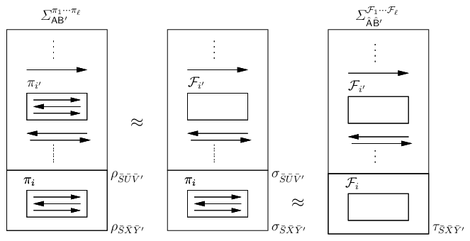
Consider now the evolution of the state when executing (as prescribed by the hybrid protocol) with a strategy for yet to be determined and when executing instead. Let and denote the corresponding states after the execution of respectively and , see Figure 2. We show that and are -close; this then proves the result by the fact that evolution does not increase the trace distance and by the triangle inequality:
Let , and be the extensions of the respective states , and when we also consider (which collects the classical communication dictated by as well as ’s classical inputs to and outputs from the previous oracle calls), which is guaranteed to exist by our formalization of a classical hybrid protocol, so that is without loss of generality contained in and . It thus follows from Proposition 2 that and are -close for a proper strategy of . Note that the strategy of may depend on the state , but since as well as ’s behavior are fixed, is also fixed.
It remains to argue that we can make independent of . We use an elegant argument due to Crépeau and Wullschleger [CW08]. We know that for any there exists a (though depending on ) as required. For any value that may take on, let then
Then, . The ’s depend on , and thus we also write . Consider now the function which maps an arbitrary distribution for to a new distribution defined as . Function is continuous and maps a non-empty, compact, convex set onto itself. Thus, by Brouwer’s Fixed Point Theorem, it must have a fixed point: a distribution with , and thus for any . It follows that which works for that particular distribution in fact works for any specific value for and so for any distribution of . ∎
6 Example: Secure Identification
We show that the information-theoretic security definition proposed by Damgård et al. for their secure-identification quantum protocol in the bounded-quantum-storage model [DFSS07] implies security in our sense for a proper functionality ; this guarantees composability as in Theorem 5.1 for their protocol. In Section 7 and in Appendix 0.B, we show the corresponding for the 1-2 OT scheme [DFR+07] and for other variants of OT.
A secure identification scheme allows a user Alice to identify herself to server Bob by securely checking whether the supplied password agrees with the one stored by Bob. Specifically, on respective input strings provided by Alice and Bob, the functionality outputs the bit to Bob. A dishonest server should learn essentially no information on beyond that he can come up with a guess for and learns whether or not, and similarly a dishonest user succeeds in convincing Bob essentially only if she guesses correctly. If her guess is incorrect then the only thing she might learn is that her guess is incorrect. The corresponding ideal functionality is depicted in Figure 3. Note that if dishonest provides the “correct” input , then allows to learn this while she may still enforce Bob to reject (by setting the “override bit” to ). In Appendix 0.C, we study a slightly stronger variant, which does not allow this somewhat unfair option for .99 9 The reason we study here the weaker version is that this corresponds to the security guaranteed by the definition proposed in [DFSS07], as we show.
Functionality : Upon receiving strings and from user Alice and from server Bob, outputs the bit to Bob.
If Alice is dishonest, then she may input an additional “override bit” . In this case, outputs the bit to Alice and the bit to Bob.
We recall the security definition from [DFSS07] for a secure identification scheme. The definition is in the framework described in Section 4.1; thus, it considers a single execution of the protocol with an arbitrary distribution for the honest players inputs and with no input for dishonest players, and security is defined by information-theoretic conditions on the resulting output states. For consistency with the above notation (and the notation used in [DFSS07]), Alice and Bob’s inputs are denoted by and , respectively, rather than and . Furthermore, note that honest Alice’s output is empty: .
Definition 2 (Secure Identification)
A password-based quantum identification scheme is -secure (against and if the following properties hold.
- Correctness:
-
For honest user Alice and honest server Bob, and for any joint input distribution , Bob learns whether their input is equal, except with probability .
- Security for Alice:
-
For any dishonest server , and for any distribution of , the resulting common output state (augmented with ) is such that there exists a classical that is independent of and such that
- Security for Bob:
-
For any dishonest user , and for any distribution of , the resulting common output state (augmented with ) is such that there exists a classical independent of , such that if then with probability at most , and
A somewhat more natural functionality (without “override bit”) can be achieved by slightly strengthening the requirements of Definition 2, see Appendix 0.C.
Proposition 3
Proof
Correctness follows immediately.
Security for Alice: Consider which is guaranteed to exist by Definition 2. Let us define and let be the bit . By the requirement of Definition 2, is independent of Alice’s input . Furthermore, we have that
by the definition of . Finally, we note that completely determines the event and therefore, we conclude using Lemma 3 that
Security for Bob: Consider which is guaranteed to exist by Definition 2. Let us define and as follows. We let where we define if , and else we choose “freshly” to be with probability and to be otherwise. Furthermore, we let . Recall that by the requirement of Definition 2, is independent of Bob’s input . Furthermore by construction, with probability , independent of the value of (and independent of whether or not). Thus, is perfectly independent of .
Since by Definition 2 the probability for Bob to decide that the inputs are equal, , does not exceed if , we have that
Finally, we have
In the case , we have by construction that and therefore, we obtain that . If , it follows from Definition 2 and the fact that is sampled independently that . Furthermore, the bit is fixed to in case and we only make an error of at most assuming that Bob’s output is always and therefore,
Putting things together, we obtain
∎
7 Another Example: Randomized 1-2 Oblivious Transfer
Figure 4 below shows the ideal functionality for sender-randomized 1-2 OT. It takes no input from Alice and an input bit from Bob, and it outputs two random -bit strings and to Alice and an -bit string which stands for the string of his choice to Bob. Note that it allows a dishonest Alice to influence the distribution of and , and a dishonest Bob to influence the distribution of ; but this is good enough for many applications, in particular to build a regular (non-randomized) 1-2 OT in the standard manner.
Functionality
Honestly behaving Alice and Bob: Upon receiving no input from Alice and a choice bit from Bob, samples two random and independent strings , and sends and to Alice and to Bob.
Honest Alice and dishonest Bob: Upon receiving no input from Alice and a bit and a string from Bob, samples a random independent string , and sends and to Alice.
Dishonest Alice and honest Bob: Upon receiving two strings from Alice and a bit from Bob, sends to Bob.
We recall the security definition of randomized 1-2 OT from [DFR+07]. The definition is in the framework described in Section 4.1 and considers a single execution of the protocol with an arbitrary distribution for honest Bob’s input bit and no input for the dishonest players. For consistency with common notation, we denote Bob’s input by (whereas Alice input is empty), and Alice’s outputs by .
Definition 3 (Rand 1-2 OT ℓ)
A randomized 1-2 OT protocol is -secure (against and ) if the following properties hold.
- Correctness:
-
If Alice and Bob are honest, then for any distribution of Bob’s input , and are -close to random and independent of , and except with probability .
- Security for Alice:
-
For any dishonest , the resulting common output state allows a classical binary such that .
- Security for Bob:
-
For any dishonest , and for any distribution of , the resulting common output state (augmented with ) allows classical such that and .
Note that the correctness condition in Definition 3 is somewhat stronger than the correctness condition in the definition proposed in [DFR+07], which merely requires that except with probability . We point out that this difference is not crucial for Proposition 4 below to hold. Indeed, if is guaranteed with high probability, then correctness as in Definition 3 can be bootstrapped from the security properties for dishonest players, albeit with some loss in the error probability: security for Bob guarantees that the distribution of is close to independent of , and security for Alice guarantees that the distribution of , which is close to the distribution of conditioned on , is random and independent of (conditioned on or not), and similar for . Working out the details is tedious1010 10 What makes it particularly tedious is that e.g. the random variable that is guaranteed to exist by the security for Alice may a-priori differ from honest Bob’s , and one has to explicitly argue that they have to be close. and does not give any new insight. In most circumstances, such an argument is not even needed. For any given protocol, the correctness condition of Definition 1 can typically be trivially verified by inspection.
Proposition 4
Proof
Correctness follows immediately.
Security for Alice: Consider which is guaranteed to exist by Definition 3. Let us define and . As Alice’s input is empty, is trivially independent of . Note that, in particular implies that . Therefore it follows that
by the definition of . Finally, by the third claim of Lemma 1, implies that
from which it follows, by Lemma 2, that
Security for Bob: Consider which is guaranteed to exist by Definition 3. Let us define and . in particular implies that . Furthermore, it is easy to see that implies
Finally, by Lemma 1, in particular implies , from which follows by Lemma 2 that . Using , this implies
The last claim follows from the following observation.
where , and similarly for . Subtracting the two terms results in a value that is upper bounded by in absolute value. ∎
8 Conclusion
We proposed a general security definition for quantum protocols in terms of simple quantum-information-theoretic conditions and showed that quantum protocols fulfilling the definition do their job as expected when used as subroutines in a larger classical protocol. The restriction to classical “outer” protocols fits our currently limited ability for executing quantum protocols, but can also be appreciated in that our security conditions pose the minimal requirements for a quantum protocol to be useful beyond running it in isolation.
Acknowledgements
We would like to thank Jürg Wullschleger for sharing a draft of [CW08] and pointing out how to avoid the dependency from the input distribution of the dishonest player in the ideal model.
References
- [BCG+05] Michael Ben-Or, Claude Crépeau, Daniel Gottesman, Avinatan Hassidim, and Adam Smith. Secure multiparty quantum computation with (only) a strict honest majority. In 46th Annual IEEE Symposium on Foundations of Computer Science (FOCS), pages 249–260, 2005.
- [BHL+05] Michael Ben-Or, Michal Horodecki, Debbie W. Leung, Dominic Mayers, and Jonathan Oppenheim. The universal composable security of quantum key distribution. In Theory of Cryptography Conference (TCC), volume 3378 of Lecture Notes in Computer Science, pages 386–406. Springer, 2005.
- [BM04] Michael Ben-Or and Dominic Mayers. General security definition and composability for quantum and classical protocols, September 2004. http://arxive.org/abs/quant-ph/0409062.
- [Cré87] Claude Crépeau. Equivalence between two flavours of oblivious transfers. In Advances in Cryptology—CRYPTO ’87, volume 293 of Lecture Notes in Computer Science. Springer, 1987.
- [CSSW06] Claude Crépeau, George Savvides, Christian Schaffner, and Jürg Wullschleger. Information-theoretic conditions for two-party secure function evaluation. In Advances in Cryptology—EUROCRYPT ’06, volume 4004 of Lecture Notes in Computer Science, pages 538–554. Springer, 2006.
- [CW08] Claude Crépeau and Jürg Wullschleger. Statistical security conditions for two-party secure function evaluation. In Third International Conference on Information Theoretic Security (ICITS), pages 86–99, 2008.
- [DFR+07] Ivan B. Damgård, Serge Fehr, Renato Renner, Louis Salvail, and Christian Schaffner. A tight high-order entropic quantum uncertainty relation with applications. In Advances in Cryptology—CRYPTO ’07, volume 4622 of Lecture Notes in Computer Science, pages 360–378. Springer, 2007.
- [DFSS05] Ivan B. Damgård, Serge Fehr, Louis Salvail, and Christian Schaffner. Cryptography in the bounded quantum-storage model. In 46th Annual IEEE Symposium on Foundations of Computer Science (FOCS), pages 449–458, 2005. Full version available at: http://arxiv.org/abs/quant-ph/0508222v2.
- [DFSS07] Ivan B. Damgård, Serge Fehr, Louis Salvail, and Christian Schaffner. Secure identification and QKD in the bounded-quantum-storage model. In Advances in Cryptology—CRYPTO ’07, volume 4622 of Lecture Notes in Computer Science, pages 342–359. Springer, 2007.
- [DFSS08] Ivan B. Damgård, Serge Fehr, Louis Salvail, and Christian Schaffner. Cryptography in the bounded-quantum-storage model. SIAM Journal on Computing, 37(6):1865–1890, 2008.
- [GL03] Daniel Gottesman and Hoi-Kwong Lo. Proof of security of quantum key distribution with two-way classical communications. IEEE Transactions on Information Theory, 49(2):457–475, 2003. http://arxiv.org/abs/quant-ph/0105121.
- [Gol04] Oded Goldreich. Foundations of Cryptography, volume II: Basic Applications. Cambridge University Press, 2004.
- [Kil88] Joe Kilian. Founding cryptography on oblivious transfer. In 20th Annual ACM Symposium on Theory of Computing (STOC), pages 20–31, 1988.
- [Kit03]
A. Kitaev.
Quantum coin-flipping.
presented at QIP’03. A review of this technique can be found in
http://lightlike.com/~carlosm/publ, 2003. - [KRBM07] Robert Koenig, Renato Renner, Andor Bariska, and Ueli Maurer. Small accessible quantum information does not imply security. Physical Review Letters, 98(140502), April 2007.
- [LC97] Hong-Kwong Lo and H. F. Chau. Is quantum bit commitment really possible? Physical Review Letters, 78(17):3410–3413, April 1997.
- [Lo97] Hong-Kwong Lo. Insecurity of quantum secure computations. Physical Review A, 56(2):1154–1162, 1997.
- [May97] Dominic Mayers. Unconditionally secure quantum bit commitment is impossible. Physical Review Letters, 78(17):3414–3417, April 1997.
- [NC00] Michael A. Nielsen and Isaac L. Chuang. Quantum Computation and Quantum Information. Cambridge university press, 2000.
- [Ren05] Renato Renner. Security of Quantum Key Distribution. PhD thesis, ETH Zürich (Switzerland), September 2005. http://arxiv.org/abs/quant-ph/0512258.
- [RK05] Renato Renner and Robert König. Universally composable privacy amplification against quantum adversaries. In Theory of Cryptography Conference (TCC), volume 3378 of Lecture Notes in Computer Science, pages 407–425. Springer, 2005.
- [Sal98] Louis Salvail. Quantum bit commitment from a physical assumption. In Advances in Cryptology—CRYPTO ’98, volume 1462 of Lecture Notes in Computer Science, pages 338–353. Springer, 1998.
- [Unr04] Dominique Unruh. Simulatable security for quantum protocols. http://arxiv.org/abs/quant-ph/0409125, 2004.
- [WST07] Stephanie Wehner, Christian Schaffner, and Barbara Terhal. Practical cryptography from noisy photonic storage. http://arxiv.org/abs/0711.2895, 2007.
- [WW08] Stephanie Wehner and Jürg Wullschleger. Composable security in the bounded-quantum-storage model. In Automata, Languages and Programming, 35th International Colloquium, ICALP 2008, volume 5126 of Lecture Notes in Computer Science, pages 604–615. Springer, 2008.
Appendix 0.A Proofs
0.A.1 Proof of Lemma 1
We show that , the first claim then follows by triangle inequality. Since quantum operations do not increase the trace distance, tracing out register in and implies that
By elementary properties of the trace distance, it follows that
The second claim follows by letting be “empty”. The third claim holds because by the triangle inequality, we have
and we can then use the second claim. ∎
0.A.2 Proof of Lemma 2
By elementary properties of the trace distance,
∎
0.A.3 Proof of Lemma 3
Let and and define the two sets and . Then,
where we used in the third equality that for , it follows from the assumption over the event that and similarly for . ∎
Appendix 0.B Other Variants of Oblivious Transfer
In this section, we give analogous “minimal” requirements for composability of other variants of oblivious transfer. It has been shown [Cré87] that all these variants of oblivious transfer are equivalent and universal for secure two-party function evaluation [Kil88]. In fact, the results of this paper show that if the variants are implemented by a quantum protocol according to our security definitions, these classical results still hold.
0.B.1 Regular (Non-Randomized) 1-2 OT
Figure 5 shows the ideal functionality for the standard (non-randomized) 1-out-of-2 String-OT. It takes two input strings and of bits each from Alice and an input bit from Bob, and it outputs an -bit string which stands for the string of his choice to Bob.
Functionality : Upon receiving from Alice and a choice bit from Bob, sends to Bob.
The definition is in the framework described in Section 4.1 and considers a single execution of the protocol with an arbitrary distribution for honest Bob’s input bit and no input for the dishonest players. For consistency with common notation, we denote Alice’s input by and Bob’s input by .
Definition 4 (1-2 OT ℓ)
A 1-2 OT protocol is -secure if the following properties hold.
- Correctness:
-
If Alice and Bob are honest, then for any joint distribution of Alice’s inputs and Bob’s input , it holds that Bob’s output except with probability .
- Security for Alice:
-
If Alice is honest, then for any dishonest Bob and any distribution of Alice’s inputs , Alice does not get any output and the common output state allows a classical binary such that and .
- Security for Bob:
-
If Bob is honest, then for any dishonest Alice and any distribution of Bob’s input , the common output state allows classical such that and .
Proposition 5
Proof
Correctness follows immediately.
Security for Alice: Consider which is guaranteed to exist by Definition 4. Let us define and . By the first requirement in the definition, we have that Alice’s input is -close to independent of .
Furthermore, it holds by definition that
Finally, by the second requirement in the definition and Lemma 2, we have that
Security for Bob: as in the proof of Proposition 4. ∎
0.B.2 Fully Randomized 1-2 OT
Figure 6 below shows the ideal functionality for fully randomized 1-2 String-OT (sometimes also called Oblivious Key OK). It takes no input from the players and outputs two random -bit strings and to Alice, a random choice bit and to Bob. Note that it allows a dishonest Alice to influence the distribution of and , and a dishonest Bob to influence the distribution of ; but this is good enough for many applications, in particular to build a regular (non-randomized) 1-2 OT in the standard manner.
Functionality :
Honestly behaving Alice and Bob: Upon receiving no input from Alice and Bob, samples two random and independent strings and a choice bit , and sends to Alice and to Bob.
Honest Alice and dishonest Bob: Upon receiving no input from Alice and a bit and a string from Bob, samples a random independent string , and sends and to Alice.
Dishonest Alice and honest Bob: Upon receiving two strings from Alice and no input from Bob, samples a random bit and sends to Bob.
The following definition is in the framework described in Section 4.1 and considers a single execution of the protocol with no inputs for honest or dishonest players. For consistency with common notation, we denote Alice’s output by and Bob’s output by .
Definition 5 (Fully Randomized 1-2 OT ℓ)
A randomized 1-2 OT protocol is -secure if the following properties hold.
- Correctness:
-
If Alice and Bob are honest, then and are -close to random and independent, and except with probability .
- Security for Alice:
-
If Alice is honest, then for any dishonest Bob, the common output state allows a classical binary such that .
- Security for Bob:
-
If Bob is honest, then for any dishonest Alice, the common output state allows classical such that and .
Proposition 6
Proof
Correctness follows immediately.
Security for Alice: as in Proposition 4.
Security for Bob: Consider which is guaranteed to exist by Definition 3. Let us define Alice’s input and Alice’s output . The requirement in particular implies that . Furthermore, it is easy to see that implies
Finally, by Lemma 1, implies , from which follows by Lemma 2 that . Using , this implies
The last claim follows from the following observation.
where , and similarly for . Subtracting the two terms results in a value that is upper bounded by in absolute value. ∎
0.B.3 Randomized Rabin OT
Figure 7 shows the ideal functionality for (randomized) Rabin Oblivious Transfer. It samples a uniform random bit and a string . It outputs to Alice, to Bob and in case , also is output to Bob. If , Bob receives the all-0 string.
Functionality :
Honestly behaving Alice and Bob: Upon receiving no input from the players, samples and and sends to Alice and to Bob.
Honest Alice and dishonest Bob: Upon receiving no input from Alice and a string from Bob, samples a random independent bit and outputs it to Bob. If , sends to Alice. If , samples a new string and sends to Alice.
Dishonest Alice and honest Bob: Upon receiving a string from Alice and no input from Bob, samples a bit and sends to Bob and no output to Alice.
The following definition is in the framework described in Section 4.1 and considers a single execution of the protocol with no inputs for honest or dishonest players. For consistency with common notation, we denote Bob’s output by .
Definition 6 (Rabin OT)
A randomized Rabin-OT protocol is -secure if the following properties hold.
- Correctness:
-
If Alice and Bob are honest, then and are -close to random and independent and except with probability .
- Security for Alice:
-
If Alice is honest, then for any dishonest Bob, the common output state allows a classical binary such that and .
- Security for Bob:
-
If Bob is honest, then for any dishonest Alice, the common output state allows a classical such that except with probability and .
Proposition 7
Proof
Correctness follows immediately.
Security for Alice: Consider which is guaranteed to exist by Definition 6. Let us define Bob’s input if . In case , sample . Let Bob’s output be . As Alice has no input , Bob’s input is trivially independent of . Furthermore, the definition requires to be -close to independent from and to completely random. In case , outputs to Bob and to Alice. In case , Bob receives and Alice’s output is independent of Bob’s input . Hence,
From follows by third claim of Lemma 1 that , and as is sampled at random, also holds. It follows that
where we used Lemma 3 for the last approximation.
Security for Bob: Consider which is guaranteed to exist by Definition 6. Let us define Alice’s input to be and let Alice’s output be empty. As Bob does not have input , Alice’s is trivially independent of . Furthermore, since is -close to uniformly random and independent of and except with probability , we have
Appendix 0.C Secure Identification without Unfairness
The goal of this section is to provide a slightly stronger functionality for secure identification than the one presented in Section 6. It is stronger in that we do not allow dishonest Alice to make Bob reject while she learns whether or not, but we still allow Alice to make Bob reject all the time by inputting a symbol that never agrees with Bob’s input, see Figure 8. In order to achieve this functionality, we have to impose a slightly stricter security definition than Definition 2.
Functionality : Upon receiving strings and from user Alice and from server Bob, outputs the bit to Bob. In case Alice is dishonest, she may choose (which never agrees with honest Bob’s input), and (for any choice of ) the bit is also output to Alice.
The definition is in the framework described in Section 4.1; thus, it considers a single execution of the protocol with an arbitrary distribution for the honest players inputs and with no input for dishonest players, and security is defined by information-theoretic conditions on the resulting output states. For consistency with the above notation (and the notation used in [DFSS07]), Alice and Bob’s inputs are denoted by and , respectively, rather than and . Furthermore, note that honest Alice’s output is empty: .
Definition 7 (Secure Identification)
A password-based quantum identification scheme is -secure if the following properties hold.
- Correctness:
-
For honest user Alice and honest server Bob, Bob learns whether their input is equal, except with probability .
- Security for Alice:
-
For any dishonest server , and for any distribution of , the resulting common output state (augmented with ) is such that there exists a classical that is independent of and such that
- Security for Bob:
-
For any dishonest user , and for any distribution of , the resulting common output state (augmented with ) is such that there exists a classical (possibly ) independent of , such that if then with probability at most , and if , Bob’s output is . Furthermore, we have that
The only difference to Definition 2 from [DFSS07] is that we additionally require for the security for Bob, that he accepts in case that . This small change allows us to achieve a more natural functionality compared to the case where we leave undefined what happens in case . We note that the protocol proposed in [DFSS07] fulfills also this strengthened Definition 7. In Step 5 of their protocol, if dishonest Alice sends a string which is inconsistent with any of the possible strings corresponding to Bob’s passwords, is set to . This is independent of and as Bob always rejects, dishonest Alice does not learn any additional information about .
Proposition 8
Proof
Correctness follows immediately.
Security for Alice: as in Proposition 3.
Security for Bob: Consider which is guaranteed to exist by Definition 7. Let and . Recall that by the requirement of Definition 7, is independent of Bob’s input .
Since by Definition 2 the probability for Bob to decide that the inputs are equal, , does not exceed if , and Bob accepts, , if , we have that
Finally, we have
In the case , we have by construction that and therefore, we obtain that . If , it follows from Definition 7 that . Furthermore, the bit is fixed to in case and we only make an error of at most assuming that Bob’s output is always and therefore,
Putting things together, we obtain
∎