Exact solution of a model DNA–inversion genetic switch with orientational control

Our model DNA inversion switch, illustrated in Fig. 1, contains three elements: the invertible DNA element and two types of recombinase enzyme ($R_{1}$ and $R_{2}$). The invertible element has two possible orientations (the “on” and “off” states). These correspond to alternative patterns of gene expression, leading to different phenotypic states; however, we model here only the core of the switch and not its downstream effects. The switch can be flipped between its two orientations by either of the recombinases. The concentration of recombinase $R_{2}$ is assumed to be fixed, while the production of $R_{1}$ depends on the switch state: $R_{1}$ is produced only in the on state. This feature of the model constitutes its orientational control and leads to its non–Poissonian behaviour. The model is represented by the following reaction scheme:

Here, $S_{\textrm{on}}$ and $S_{\textrm{off}}$ denote the on and off states of the switch. Reactions (1a) describe the production and decay of recombinase $R_{1}$: $R_{1}$ is removed from the system with rate constant $k_{1}$ (due to cell growth and division, which we do not model explicitly), and is produced at rate $k_{2}$ only when the switch is in the on state. Reactions (1b) describe switch flipping. This may be catalysed by $R_{1}$ with rate constants $k^{\textrm{on}}_{3}$ (on to off) and $k^{\textrm{off}}_{3}$ (off to on). We shall mainly consider here the case $k^{\textrm{off}}_{3}=0$. Recombinase $R_{2}$ can also catalyse switch flipping. The concentration of $R_{2}$ (fixed in our model) is not explicitly included in the reaction scheme, but is implicit through a dependence of the rate constants $k_{4}^{\textrm{on}/\textrm{off}}$ on the $R_{2}$ concentration.

We note that mean-field, macroscopic rate equations corresponding to the above reaction scheme yield only one steady-state solution corresponding to the average switch state and average concentration of $R_{1}$. The underlying deterministic structure of the model is thus not bistable. In this sense, our model is fundamentally different from the bistable reaction networks presented in [6, 7, 8].

Our model is inspired by the fim genetic regulatory system [3]. In analogy with fim, $R_{1}$ in our model represents FimE while $R_{2}$ represents FimB. Environmental stimuli such as nutrient conditions and temperature act on the fim switch largely through changes in the level of FimB [9, 10]; this would correspond to variation of our key parameters $k_{4}^{\textrm{on}/\textrm{off}}$. However, our model is highly simplified in comparison to fim, in that it neglects cooperative and competitive recombinase binding and the effects of other DNA binding proteins. Our objective in this work is not to model the details of the fim system, as other authors have done [9, 10], but rather to address general questions about the behaviour of this type of switch. Our model is designed to be as simple as possible while retaining the key features of DNA inversion and orientational control; its simplicity allows us to obtain analytical results and to explore a wide range of parameter space.

We simulated the reaction scheme (1) using a continuous time Monte Carlo scheme [11]. A typical trajectory is shown in Fig. 1, where we plot the number $n$ of $R_{1}$ molecules and the switch state as functions of time. When the switch is in the on state, $n$ increases (on average) towards a plateau value of $k_{2}/k_{1}$, while in the off state $n$ decays towards zero. We now obtain an exact analytical solution for the case where $k^{\textrm{off}}_{3}=0$. This case is relevant to the fim switch, where FimE catalyses almost exclusively on to off switching. In the following, all our analytical results will correspond to $k^{\textrm{off}}_{3}=0$, while simulation results will be presented also for $k^{\textrm{off}}_{3}>0$. Analytical results for $k^{\textrm{off}}_{3}>0$ will be published elsewhere.

We first consider the statistics of $n$ in the steady state and compute the long time, joint probability $p_{s}(n)$ that the switch is in state $s$ and there are $n$ molecules of $R_{1}$. The system of birth–death equations for $p_{\textrm{on}}(n)$ and $p_{\textrm{off}}(n)$ becomes in the steady state

In order to decouple the above set of equations, we solve (2a) for $p_{\textrm{off}}$, then insert the result into (2b) to give a decoupled equation for $p_{\textrm{on}}$. Introducing the generating function $G_{s}(z)=\sum_{n}z^{n}p_{s}(n)$ (where $s=\{\textrm{on},\textrm{off}\}$), the decoupled equation for $p_{\textrm{on}}$ reduces to a second order differential equation for $G_{\textrm{on}}$. Defining then a new variable $u\equiv u_{z}=k_{2}z/(k_{1}+k^{\textrm{on}}_{3})-k_{1}k_{2}/(k_{1}+k^{\textrm{on}}_{3})^{2}$, the latter equation reads:

where $a=1+u_{1}+(k^{\textrm{on}}_{4}+k^{\textrm{off}}_{4})/(k_{1}+k^{\textrm{on}}_{3})$ and $b=1+k^{\textrm{off}}_{4}/k_{1}$. Expanding the solution as a regular power series (i.e. $G_{\textrm{on}}(u)=\sum_{m}a_{m}u^{m}$), one finds that $G_{\textrm{on}}(z)=a_{0}\,{{}_{1}F_{1}}(b,a,u)$, where ${}_{1}F_{1}$ is a confluent hypergeometric function and $a_{0}$ is an integration constant which can be determined with the normalisation condition $\sum_{n}p_{\textrm{on}}(n)+p_{\textrm{off}}(n)=1$ (or equivalently $G_{\textrm{on}}(1)+G_{\textrm{off}}(1)=1$). This result can be rewritten in terms of the original variable $n$ as

where $(\alpha)_{n}=\alpha(\alpha+1)\dots(\alpha+n-1)$. An expression for $p_{\textrm{off}}$ can be derived by inserting Eq.(4) into Eq. (2a). In Fig.2 we compare the result for $p(n)=p_{\textrm{on}}+p_{\textrm{off}}$ to simulations, obtaining perfect agreement.

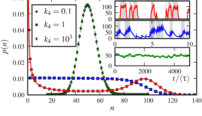
Figure 2 also illustrates the effects of the different timescales for switch flipping and production/decay of $R_{1}$. For small $k_{4}$, switch flipping is slow compared to the rate of change of $n$. In this case, when the switch is in the on state, the number of recombinase has time to reach a plateau before the switch flips off. The on and off switch states are then each associated with a different value of $n$ and the distribution $p(n)$ is bimodal. In contrast, when $k_{4}$ is large, the switch flips back and forth much more rapidly than recombinase production or removal. Then, the fraction of time spent in the on state is $k_{4}^{\textrm{off}}/(k_{4}^{\textrm{off}}+k_{4}^{\textrm{on}})$, and $p(n)$ tends to the Poisson distribution expected for a birth-death process with birth rate $k_{2}^{\textrm{on}}k_{4}^{\textrm{off}}/(k_{4}^{\textrm{off}}+k_{4}^{\textrm{on}})$ and death rate $k_{1}$.

To determine how orientational control affects switch function, we compute flipping time distributions. The flipping time $T$ can be defined in two different ways. In the first scenario, which we call the Switch Change Ensemble (SCE), we define $T$ as the time spent in a particular switch state—for example, $F_{\textrm{on}}^{\textrm{SCE}}(T)$ is the probability distribution for the time between the moment the switch enters the on state and the moment it flips from the on to the off state. In the second scenario, which we call the Steady State Ensemble (SSE), we start observing the cell at a random moment and measure the time interval between this moment and its next flip into the other state. $F_{\textrm{on}}^{\textrm{SSE}}(T)$ and $F_{\textrm{off}}^{\textrm{SSE}}(T)$ may be relevant to the response of a population of switching cells to a sudden environmental change. They also correspond to an experiment where one measures the time until the next flip, for cells sampled in the steady state [12]. To compute these distributions, we define $F_{s}(T|n_{0})$ as the probability that the system begins at $t=0$ in the $s$ state with $n_{0}$ recombinase and flips for the first time at $T$. Note that for $k^{\textrm{off}}_{3}=0$, the off to on flipping process does not depend on $R_{1}$ and is governed by $k_{4}^{\textrm{off}}$; thus $F_{\textrm{off}}(T)=k^{\textrm{off}}_{4}\exp(-k^{\textrm{off}}_{4}T)$ is independent of $n_{0}$ (for both the SCE and the SSE). However, the on to off flipping rate is $n_{0}$ dependent, so that we average over the ensemble of initial states (characterised by the probability $W_{\textrm{on}}(n)$ of having $n$ recombinase at the start of our measurement) to obtain the flip time distribution $F_{\textrm{on}}(T)=\sum_{n_{0}}W_{\textrm{on}}(n_{0})F_{\textrm{on}}(T|n_{0})$. For the SCE, the initial condition is taken just after a flip, which implies that $W_{\textrm{on}}^{\textrm{SCE}}(n_{0})=p_{\textrm{off}}(n_{0})/G_{\textrm{off}}(1)$. For the SSE, the initial condition is sampled in the steady state, yielding $W_{\textrm{on}}^{\textrm{SSE}}(n_{0})=p_{\textrm{on}}(n_{0})/G_{\textrm{on}}(1)$. To compute $F_{\textrm{on}}(T)$, we first define the survival probability $h_{\textrm{on}}(n,t)$ that, at time $t$, the switch is in the on state with $n$ $R_{1}$ molecules, without having flipped, given the initial condition $h_{\textrm{on}}(n_{0},0)=W_{\textrm{on}}(n_{0})$. The evolution equation for $h_{\textrm{on}}$ is:

Defining a generating function ${\tilde{h}}_{\textrm{on}}(z,t)=\sum_{n}z^{n}h_{\textrm{on}}(n,t)$, it follows that $F_{\textrm{on}}(t)=-\partial_{t}{\tilde{h}}_{\textrm{on}}(1,t)$. Eq.(5) reduces to a partial differential equation for ${\tilde{h}}_{\textrm{on}}(z,t)$ which has the initial condition ${\tilde{h}}_{\textrm{on}}(z,0)=\sum_{n_{0}}W_{\textrm{on}}(n_{0})z^{n_{0}}$. Its solution is

where $\tau_{\textrm{on}}=(k_{1}+k^{\textrm{on}}_{3})^{-1}$. $F_{\textrm{on}}(T)$ can then be computed for the different measurement scenarios using ${\tilde{h}}_{\textrm{on}}(x,0)=G_{s}(x)/G_{s}(1)$ with $s={\rm off}$ for SCE and $s={\rm on}$ for SSE.

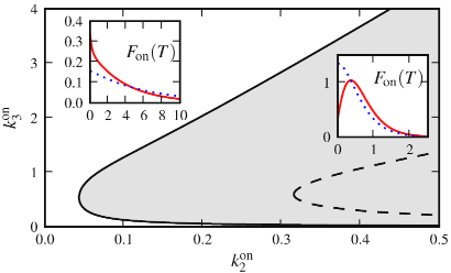
Our results, illustrated in Fig.3, show a striking effect of orientational control for this model switch: for the SCE, we can obtain a peak in the flipping time distribution. Such a peak has been postulated for the fim switch [9], where it might imply that the switch tends not to leave the on state before it has had time to synthesise fimbriae [9, 10, 3]. Time spent in the on state may also influence recognition by the host immune system. This peak in $F_{\textrm{on}}^{\textrm{SCE}}$ is a consequence of the feedback between the switch state and the level of $R_{1}$. Once in the on state, the rate of on to off flipping increases with time as $R_{1}$ is produced. In contrast, for a Poissonian switch, the rate of flipping is constant in time. For a peak to occur, the slope of $F_{\textrm{on}}^{\textrm{SCE}}$ at the origin must be positive, which implies

where $\left\langle\dots\right\rangle$ denotes an average using the weight $W_{\textrm{on}}$. The l.h.s. of (7) can be evaluated numerically using the exact result (4) to compute $\langle n_{0}\rangle$ and $\langle n^{2}_{0}\rangle$. We can then determine the regions of parameter space where a peak exists, as shown in the shaded region of Fig. 3 for the SCE. Our results show that the presence of a peak is favoured by large values of $k_{2}$ (strong production of $R_{1}$ in the on state), and suppressed by very large values of $k^{\textrm{on}}_{3}$ (strong $R_{1}$–mediated on to off switching) or by very small values of $k^{\textrm{on}}_{3}$ (switching dominated by $R_{1}$–independent mechanism). Likewise, when $k_{4}$ is increased, the range of values over which the peak exists is decreased, since $R_{1}$–independent Poissonian switching tends to dominate. For the SSE, on the other hand, we did not find any parameter values where inequality (7) is verified. The peak in the SCE appears because the number of recombinase, and hence the flipping probability, is typically low immediately after entering the on state and increases significantly thereafter. In contrast, in the SSE one typically starts a measurement when $n$, and hence the flipping probability, is already high. This tends to suppress the peak in the SSE flipping time distribution.

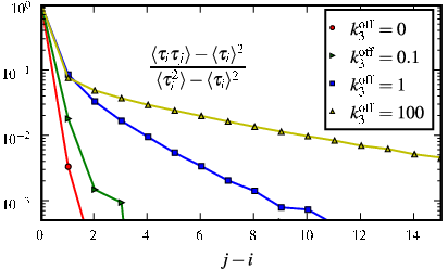
Another potentially important effect of the feedback between the switch state and the production of recombinase $R_{1}$ may be to cause correlations in the waiting times between successive flips (for example, a particularly short time before a flip might lead to subsequent flips occurring in quick succession). Such correlations might allow a population of switching microbes to “remember” the history of past environmental changes. We define the switch period $\tau_{i}$ as the time from when the switch enters the on state from the off state for the $i$th time, until it enters the on state for the $(i+1)$th time [cf. Fig. 1]). In Fig. 4, we plot simulation results for the correlation function for switch periods $\tau_{i}$ and $\tau_{j}$ , as a function of $j-i$. For $k^{\textrm{off}}_{3}=0$, weak correlation is observed between subsequent periods $\tau_{i}$ and $\tau_{i+1}$. Correlations are weak because when $k^{\textrm{off}}_{3}=0$, the off to on switching process does not depend on $R_{1}$ and is an uncorrelated Poisson process. When $k^{\textrm{off}}_{3}\neq 0$, correlations are much stronger and extended correlated sequences of flips emerge.

We have presented a generic model for a DNA inversion switch with orientational control. By solving the model analytically in the case $k_{3}^{\textrm{off}}=0$ (relevant to the fim switch), and using stochastic simulations, we have shown that this type of switch can display markedly non–Poissonian behaviour, including a peaked flipping time distribution for intermediate values of $k^{\textrm{on}}_{3}$ and, for $k_{3}^{\textrm{off}}>0$, correlated sequences of flips. Non–Poissonian behaviour has been postulated to be a consequence of orientational control [3, 9]. The model presented here allows us to analyse the origins and effects of this behaviour in detail, and provides analytical results which can be used as a basis for more complex models [13]. Suggested evolutionary roles for orientational control include rapid response to environmental change [10], as well as peaked flipping time distributions [3, 9]. This study raises interesting questions about the consequences of non–Poissonian switching for population dynamics in changing environments. Several models have been proposed for the growth of populations of switching cells in stochastically and periodically changing environments (see, for example [14]). These models assume Poissonian switch flipping. The analytical solutions presented here should make it possible to extend such models to the case of non-Poissonian flips. Non-Poissonian switch flipping opens up the possibility that lineages of cells may ‘remember’ (in a statistical sense) the history of their recent phenotypic states. This is likely to have important consequences for models which include selection according to the fitness of different phenotypic states in changing environments. We speculate that bacteria which adopt a non-Poissonian flipping strategy may be able to maximise the evolutionary advantages of using some knowledge of the likely future behaviour of the environment, combined with the benefits of a stochastic strategy as an insurance against sudden and unpredictable environmental changes. These avenues will be the subject of future work.