Electronic Structure in Gapped Graphene with Coulomb Potential
Abstract
In this paper, we numerically study the bound electron states induced by long range Coulomb impurity in gapped graphene and the quasi-bound states in supercritical region based on the lattice model. We present a detailed comparison between our numerical simulations and the prediction of the continuum model which is described by the Dirac equation in ()-dimensional Quantum Electrodynamics (QED). We also use the Fano’s formalism to investigate the quasi-bound state development and design an accessible experiments to test the decay of the supercritical vacuum in the gapped graphene.
pacs
81.05.Uw, 71.55.-i, 71.23.-kIntroduction Graphene, a two-dimension (2D) hexagonal lattice of carbon atoms, exhibits special electronic dispersion relation, in which electrons behave like massless relativistic Dirac fermions [1, 2, 3]. This special property leads to many unconventional phenomena, such as the Klein paradox[4] and the Vaselago lensing effect[5]. Due to its large ”fine structural constant”, graphene not only provides an exciting platform to validate some predictions of Quantum Electrodynamics (QED) in the strong field, but also provides an interesting ”strong coupling” 2+1 QED model[6].
Recently, it was found that a substrate induced potential can break the chiral symmetries of massless Dirac equation and generate gaps in graphene electron spectrum[7]. The motion of electrons, therefore, can be described by massive 2D Dirac equations. It was predicted that a Coulomb charged impurity in gapped graphene behaves the same as the heavy-atom in the QED theory. The charged impurities have a significant effect on the electronic structures of the gapped graphene [8, 9, 10, 11, 12]. Depending on the charge , the bound states can be induced inside the gap, and the quasi-bound states can also be generated when the charge is sufficiently larger than the supercritical number . If the energy of bound state is above the middle of the gap, the wave function of bound electron state in the pure Coulomb potential can be well determined by using the continuum model. If the energy of bound state is below the middle of the gap, the wave function of bound state, however, cannot be well described because of the singular nature of the pure Coulomb potential near . To solve this problem, a rough but simple approximation is adopted to remove this singularity condition by taking into account the finite spatial extension of nuclear charge with radius based on 3+1 QED model [13]. When a continuum model is used to describe the behavior of electrons in graphene near the Dirac point, in fact, how to choose the boundary condition is still an open question. For example, Ref.[14] chose a “Zigzag edge” boundary condition to discuss the vacuum polarization in gapless graphene, but Ref.[15] used an “infinite mass” boundary condition. This situation, however, dose not exist in the tight-binding model due to its lattice scale cutoff.
In this paper, based on the lattice model, we use the tight-binding approach to numerically calculate the electronic structure in gapped graphene. From the results of local density of states (LDOS), we discover that the energy position of bound states can be determined within the non-supercritical region, and supercritical charge can also be determined using the continuum model and the lattice model. We also discuss the relationship between the gap and critical charge . Finally, we use the description of resonances to explain the quasi-bound state development in a supercritical regime.
The Lattice Model and Continuum Model In what follows, we consider a single attractive Coulomb impurity placed at the center of a honeycomb lattice in a graphene sheet. The corresponding Hamiltonian in the tight-binding form is:
| (1) |
where is hopping energy between the nearest neighbor atoms. The operator () and () denote creation (annihilation) an electron on the sublattice A and sublattice B, respectively. The first term of Hamiltonian describes the hopping between the nearest neighbor atoms. The second term is the on-site energy of sublattice A and sublattice B. corresponds to the mass (or the gap) of Dirac fermions. It is well known that the non-zero mass term can open a wide gap within the band spectrum. Many conditions can lead to a band-gap within graphene. For instance, Ref[7] reports that the SiC substrate can open a gap of in a single-layer graphene, which is consistent with the calculation of the first principle [16]. In our calculations, we select from (or eV) to (or eV). reflects the impurity charge strength and is the effective dielectric constant. When energy level is close to the Dirac point, the Hamiltonian in gapped graphene can be approximately described by a continuum model:
| (2) |
where are the Pauli matrices. We can view as “fine structural constant” in graphene. is the Fermi velocity of graphene and . is the mass of the Dirac fermion. Since is sufficiently small compared with the velocity of light in the QED theory, then becomes much larger than that in the QED theory. The large value of ”fine structural constant” of graphene means that the perturbation expansion, which works well in QED, can not directly apply to discuss the many body problems in graphene .
Bound states above the middle gap In the continuum model, the eigenfunction of a pure Coulomb potential can be described by the confluent hypergeometric function [14, 17]. The regularity at and requires the confluent hypergeometric functions reduce to polynomials at the same time. Energy of the bound states within the gap , as a result, satisfies the following condition:
| (3) |
with the root . Here and takes an integer value and half of an integer, respectively. That is, and . is the isospin-orbital momentum number [17]. Non-supercritical region is defined because is always real for all angular momentum channels. If the control charge exceeds the value , the solutions of the continuum model break down since the root becomes imaginary. Hence, all bound states below the middle of gap do not exist. This artifact can be remedied by removing the singular behavior of the pure Coulomb potential. When the energy of the bound state above the middle of gap, one can see from Eq. that the energy of the bound state is linearly proportion with the gap width, and the lowest bound state reaches the middle of the gap at a critical value that satisfies .
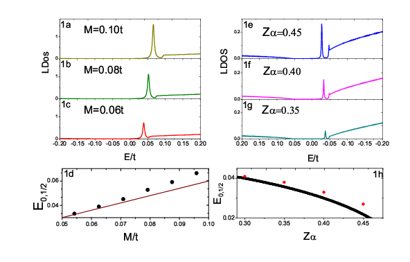
As shown in Fig.1, the LDOS spectrum for the bound state above the middle gap is calculated numerically by the tight-binding approach. By fixing the electromagnetic coupling , we can plot the LDOS spectrum of the bound states with different gap widthes () as shown in Fig. 1a to Fig. 1c. Except that the lowest bound states ( and ) in the gap can be clearly resolved based on the LDOS spectrum, the other bound states are very close to the edge of the positive energy continuum and thus one cannot clearly distinguish them from Fig.1a to Fig.1c. The energy of the lowest bound state is plotted in Fig.1d as a function of the gap width. The dotted line is depicted based on our numerical simulations in the lattice model. The theoretical results is also plotted by using the equation of the continuum model. When the gap width is not too large, the energy of the lowest bound state calculated by the numerical simulation show a slightly deviation away with that predicted by the continuum model. As the gap increases, the deviation becomes larger.
If the gap width is set to be , Fig1.e to Fig.1g illustrate the LDOS spectrum of the bound states with different chosen electromagnetic coupling factor, . The peak of LDOS corresponding to the lowest bound state gets close to the middle gap as increases. Fig. 1h plots the energy of the lowest bound state as a function of . The dotted line gives the result of numerical simulations and the fitting curve is plotted using equation (3) of the continuum model. The numerical simulations fit Eq. () well when is small. Fig. 1h also imply that the electromagnetic coupling needs to be larger than in order to make the energy of the lowest bound state to reach the middle of the gap.
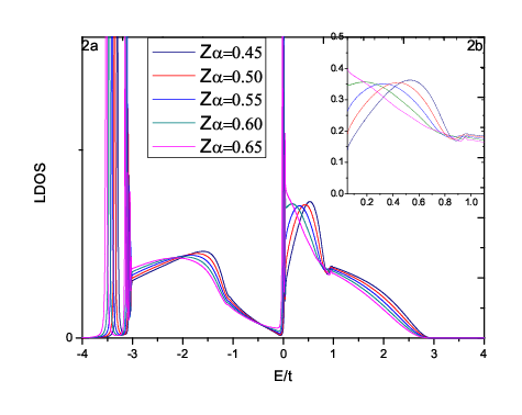
The effect of Coulomb charge on energy continuum is shown in Fig.2. Except for the existent of bound states in the gap, the main feathers of the LDOS spectrum on gapped graphene is almost the same as that in the gapless graphene [15]. The strong re-normalization of the van Hove singularities are also observed.[15]. Note that the LDOS spectrum near the edge of positive energy continuum appears some interesting physical signature, which is discussed in the following.
Bound states below the middle gap The Dirac equation with the pure Coulomb potential can only provide the solution of bound state above the middle of gap. When exceeds , becomes imaginary in this continuum model, which does not have a regular solution. For the pure Coulomb potential, the continuum model points out that this is critical point when equals . In the lattice model, the bound state, however, can be gradually enter the energy region below the middle of gap as increases. Thus, this point seems not critical. In this paper, for a convenient comparison between the results obtained by the lattice model and by the continuum model, we still define a critical value which represents the energy of the lowest bound state just touches the middle of gap . More interesting, our numerical simulations reflect that some physical signatures are associated to this point.
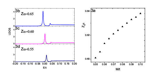
Fig.3b Fig.3d show the situation that the bound states enter below the middle of gap when we fix the gap width . The bound states exist below the middle gap as the increases. The relationship between the critical charge and the gap width is numerically calculated and the results are shown in Fig.3a. The trigonal dots stands for the numerical results of critical charge . Therefore, the value depends on the gap width in our lattice model. For example, the critical value is about when the gap width is . It is more interesting to note that there still exist some physical signatures related to this critical value. As shown in Fig.2b, the LDOS spectrums of the positive energy continuum near the gap appear significantly different for versus . When , the LDOS of positive energy continuum decreases as gets close to the gap region. However, for , the LDOS of positive energy continuum near the gap is almost independent of . When , the LDOS spectrum near the gap appears an increasing trend as decreases. The physics behind this phenomenon needs to be explained in our future research.
Supercritical Region and the Decay of Vacuum As continues to increase, the energy of the lowest bound state becomes close to the edge of band gap (). When is sufficiently larger than the critical value , the energy of bound state will drop into the negative continuum spectrum. In this case, the bound state changes its characteristics and becomes a quasi-bound state. As predicted by the QED theory[13], the neutral vacuum changes into the charged vacuum. The processes with this change is called the decay of vacuum. We first calculate the supercritical charge in gapped graphene by using the continuum model and the lattice model, respectively. To determine the diving point by the continuum model, one needs to remove the singular behavior of the pure Coulomb potential. A simple choice is that the potential takes the form , and , otherwise. Hence, the supercritical charge for the lowest bound state can be determined through the boundary condition at [13, 18]:
| (4) |
where and . This is a transcendental equation for and the numerical result gives at . If the gap width is set to be , the corresponding equals about .
Based on our lattice model, Fig.4a shows the numerical results when the lowest bound state enters into the negative energy continuum. The results indicate that the supercritical charge is about when . Inset in fig.4a reflects the relationship between and the gap width . The square dots represents the numerical results based on the lattice model. The fitting line implies that depends linearly on the gap width , which satisfies the result of the above transcendental equation , when .
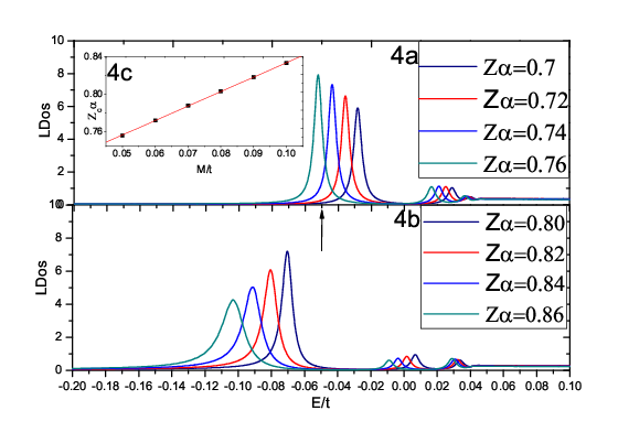
If , the lowest bound state enters the negative energy continuum and becomes a resonant state. The LDOS spectrum clearly shows the resonant state in negative energy continuum (refer to Fig.4b). The LDOS spectrum also shows that the second lowest bound state is distinguishable. From the numerical results, we can see that the width of quasi-bound state becomes large as increases. This behavior can be explained by the method developed by U. Fano for the auto-ionization of excited states in Atomic Physics. We assume that new continuum wave function in the supercritical region can be expanded as [19], where and represent the discrete eigenstate and the continuous spectrum when . If exceeds , can be considered as a perturbation potential. On the boundary of the supercritical region, we can simply revise the results in Ref.[19]:
| (5) |
where and . The LDOS is defined as [14]. We obtain that relates to as . depends linearly on additional Coulomb charge while width of the quasi-bound quadratically increases with the additional Coulomb charge. These observations is consistent with our numerical results qualitively as shown in fig.4b.
Particularly important, some gedanken experiments were proposed to test the interesting physical process related to the supercritical vacuum.[13] For example, the feature of the spectrum of the emitted positron depending on the ”critical duration” which reflects the decay of the supercritical vacuum. Unfortunately, there still exist difficulty to perform this experiment in QED. Since “the Compton wavelength ” in gapped graphene is sufficiently large comparing with that in QED, one can use the gating technique to design experiments to measure the decay of the supercritical vacuum in a gapped graphene.
Summary In this paper, considering the contribution of the long-range Coulomb impurity in gapped graphene, we numerically calculate the LDOS spectrum using the lattice model. The relationship between the critical value and gap is investigated, which corresponds to the lowest bound state at the middle gap or at the diving point, respectively. We also compare the numerical simulation results of the lattice model with that of the continuum model. The width of quasi-bound state is explained by the Fano’s formulism.
Noted added. While preparing this manuscript, we were aware of preprint[20] that has some overlapping with this paper.
Acknowledgement This work is partially supported by the National Natural Science Foundation of China (Grant nos. 10574119). The research is also supported by National Key Basic Research Program under Grant No. 2006CB922000. Jie Chen would like to acknowledge the funding support from the Discovery program of Natural Sciences and Engineering Research Council of Canada under Grant No. 245680.
References
- [1] K.S. Novoselov et al., Science 306, 666 (2004).
- [2] K.S. Novoselov et al., Nature 438, 197 (2005).
- [3] A. Geim et al., Nature Mater. 6, 183 (2007).
- [4] M.I. Katsnelson et al., Nature physics 2, 620 (2006).
- [5] Vadim V. Cheianov et al., Science 315, 1252 (2007)
- [6] T. Applequest et al., Phys. Rev. Lett. 60, 2575 (1988)
- [7] S.Y. Zhou et al., Nature Mater. 6, 770 (2007).
- [8] T.O. Wehling et al, Phys. Rev. B. 75, 125425 2007
- [9] A.H. Castro et al, Cond-mat 07091163
- [10] Yu. V. Skrypnyk et al, Phys. Rev. B. 73, 241402(R) (2006)
- [11] Vitor M. Pereira et al., Phys. Rev. Lett. 96, 036801 (2006)
- [12] P. M. Ostrovsky et al, Phys. Rev. B. 74, 235443 (2006)
- [13] Greiner, Quantum electrodybamics, third edition. (2000)
- [14] A.V.Shytov et al., Phys. Rev. Lett. 99, 236801 (2007).
- [15] Vitor M. Pereira et al., Phys. Rev. Lett. 99, 166802 (2006).
- [16] F. Varvhon et al., Phys. Rev. Lett. 99, 126805 (2007).
- [17] D.S. Novikov et al., Phys. Rev. B. 76, 245435 (2006).
- [18] V.R. Khalilov, et al.,hep-th/9801012
- [19] J. Reinhardt et al., Rep. Prog. Phys. 40, 219 (1977).
- [20] V. M. Pereira et al.,Cond-mat 0803-4195