Continuum theory of memory effect in crack patterns of drying pastes

First, we review the Lagrangian description of kinematics. The configuration of an ${n_{\text{d}}}$-dimensional continuum is represented by a mapping from Lagrangian variable $\bm{\xi}$ (also known as “label” or “material variable” [16]) to the position vector $\mathbf{r}$. For ${n_{\text{d}}}=3$, we write

where $\left[\quad\right]_{\text{C}}$ denotes the representation in terms of Cartesian components. For ${n_{\text{d}}}=2$ we will omit $\eta$ and $y$, assuming that all the motion occurs in the $(x,z)$-plane.

The time-derivative of $\mathbf{r}=\mathbf{r}(\bm{\xi},t)$ gives the velocity,

In Eq. (6) and in what follows, $\partial_{t}$ stands for the time-derivative in the Lagrangian description (Lagrange derivative, which is usually denoted by $\mathrm{D}/{\mathrm{D}t}$ in Eulerian description). Using $\left\{{\partial_{\xi}}\mathbf{r},{\partial_{\eta}}\mathbf{r},{\partial_{\zeta}}\mathbf{r}\right\}$ (where ${\partial_{i}}=\partial/{\partial{\xi^{i}}}$) as the set of local bases, we can represent the velocity as

In Eq. (7) and in what follows, summation over $i\in\{\xi,\eta,\zeta\}$ is understood according to Einstein’s contraction rule. The coefficients $(v^{i})$ in Eq. (7) are referred to as the contravariant components of $\mathbf{v}$ (see Eqs. (59) and (64) in Appendix A). The acceleration is $\partial_{t}\mathbf{v}=\partial_{t}\left(v^{i}{\partial_{i}}\mathbf{r}\right)$; we emphasize again that $\partial_{t}$ denotes the Lagrange derivative.

The square of the Euclidean distance between two neighboring “particles,” labeled by $\bm{\xi}$ and $\bm{\xi}+\mathrm{d}\bm{\xi}$, is

which introduces the metric tensor denoted by $(g_{ij})$ or $\mathsf{g}$. In this paper we refer to $\mathsf{g}$ as the “Euclidean” metric tensor, which does not mean that $g_{ij}$ is equal to Kronecker’s delta but means that the Euclidean metric of the $\mathbf{r}$-space is imported into the $\bm{\xi}$-space by Eq. (8).

In general, it is totally unnecessary to choose $\bm{\xi}$ to be some “initial” position of the element, except for some particular situations in which the initial state has a special significance. One of these special cases is that of purely elastic bodies initially set in a stress-free and undeformed state, called a “natural state” [17]. It is meaningful in this case to choose the “natural state” position vector as $\bm{\xi}$ so that $g_{ij}$ defined by Eq. (8) is essentially identical to the Cauchy-Green deformation tensor [9] whose difference from $\delta_{ij}$ is responsible for the elastic restoring force. This is a rather special case, however. More generally, $\bm{\xi}$ has nothing to do with the initial state, and the natural metric tensor $\mathsf{g}^{\natural}$ is used as a reference to define the elastic deformation, instead of assuming the global existence of the stress-free natural state. The (locally) undeformed state is formulated as $\mathsf{g}=\mathsf{g}^{\natural}$, and the difference between $\mathsf{g}$ and $\mathsf{g}^{\natural}$ is responsible for the stress. More details about $\mathsf{g}^{\natural}$ will be discussed later.

The incompressibility condition is expressed as

because the mass of a fluid element is $\rho\sqrt{\det{\mathsf{g}}}\,{\mathrm{d}^{{n_{\text{d}}}}\bm{\xi}}$ which should remain unchanged, and the density $\rho$ also remains unchanged during the motion. For simplicity, we assume that $\rho$ is a global constant. Then, without loss of generality, we can replace Eq. (9) by

Now we detail the dynamics. With the stress field denoted by $\mathsf{P}=P^{ij}({\partial_{i}}\mathbf{r})\otimes({\partial_{j}}\mathbf{r})$ and the external body force by $\mathbf{F}=F^{i}{\partial_{i}}\mathbf{r}$, the momentum equation is written as

or, in contravariant component representation, as [17]

The left-hand side is the contravariant component of the acceleration vector $\partial_{t}\mathbf{v}$ multiplied by the density $\rho$, and $\nabla_{j}$ denotes the covariant derivative (these mathematical concepts are clarified in Appendix A to the degree sufficient for the present work; for a more profound understanding of the mathematical background, see Refs. [17, 18]). While $\mathbf{F}$ is regarded as given, $\mathsf{P}$ must be determined by a suitable constitutive relation.

From the discussion in the previous section, we expect that $\mathsf{P}$ obeys a viscoelastic equation of Maxwell type. The Maxwell model is often illustrated as a spring and dashpot connected in series [9], for which the relation between the tension $T$ and the total length $x$ is given by

where $\kappa$ is the spring constant, $\mu$ is the resistance, $x_{\text{S}}$ and $x_{\text{D}}$ are the length of the spring part and the dashpot part, respectively, and $x_{\text{S}}^{\natural}$ denotes the natural length of the spring part. It is customary to eliminate the “internal” variables ($x_{\text{S}}$, $x_{\text{D}}$ and $x_{\text{S}}^{\natural}$) from Eq. (12), which yields

A timescale $\mu/\kappa$ in regard to stress relaxation is recognized in Eq. (13).

Now it is necessary to elaborate the Maxwell model in two respects: it needs to include plasticity and it also needs to describe ${n_{\text{d}}}$-dimensional continuum mechanics. In regard to the first point, most of the existing studies are based on an elasto-plastic decomposition, which is a direct extension of Eq. (12). However, this approach has a disadvantage in that the incautious use of internal variables can lead to a difficulty, in particular for a finite deformation [19, 20]. Here we adopt a different approach that is closer to Eq. (13), thereby avoiding a direct reference to the internal variable $x_{\text{D}}$.

The essential idea is to attribute the relaxation to the natural length $x^{\natural}$, which is related to the tension $T$ as if the model is totally elastic:

The natural length $x^{\natural}$ can be expressed as $x^{\natural}=x_{\text{S}}^{\natural}+x_{\text{D}}$ in terms of internal variables, but this relation is not to be used explicitly; we note only that $x^{\natural}$ is time-dependent while $x_{\text{S}}^{\natural}$ is not. By substituting Eq. (14) into Eq. (13), we find an equation that describes the relaxation of the natural length $x^{\natural}$:

Eqs. (14) and (15) provide us with a prototype of the plastic model.

Let us find ${n_{\text{d}}}$-dimensional continuum equations corresponding to the prototypical equations (14) and (15). As a candidate, we adopt an elastic constitutive equation

together with an inelastic equation

where $(g^{ij})$ denotes the inverse of the component matrix of the “Euclidean” metric tensor $(g_{ij})$, and $(g_{\natural}^{ij})$ is that of the natural metric tensor, such that

The natural metric tensor $\mathsf{g}^{\natural}$ represents the square of the “natural distance” between two neighboring points labeled by $\bm{\xi}$ and $\bm{\xi}+\mathrm{d}\bm{\xi}$,

in the sense that the difference between $\mathrm{d}{s}^{2}$ and $\left({\mathrm{d}{s}^{\natural}}\right)^{2}$ accounts for the restoring force according to Eq. (16). In the special case of purely elastic bodies initially set in a stress-free “natural state” (at $t=t_{0}$), $\mathrm{d}{s}^{\natural}$ is the distance in this initial configuration and $\mathsf{g}^{\natural}$ is the corresponding metric:

In general, however, $\mathsf{g}^{\natural}$ differs from the initial value of $\mathsf{g}$. This is inevitable due to Eq. (17), which prescribes that the natural metric $\mathsf{g}^{\natural}$ is subject to relaxation. To make Eq. (17) more easily recognizable as a relaxation equation, we rewrite it in the manner of Eqs. (2) and (15b) as

this equation provides that $(g_{\natural}^{ij})$ should evolve toward an isotropic tensor $(Kg^{ij})$. Plasticity is incorporated via $\tau$ according to Eq. (1). The idea of using a natural metric to reformulate the Maxwell model has been known among several researchers of rheology (including the authors of Refs. [11, 12]), but the present author could not identify any publications in which the notion of the natural metric and its relaxation is formulated explicitly.

The ${n_{\text{d}}}$-dimensional elastic equation (16), corresponding to the one-dimensional Hookian equation (14), originates from consideration of elastic strain energy. Since $g^{\natural}_{ij}\mathrm{d}\xi^{i}\mathrm{d}\xi^{j}$ is a positive definite quadratic form, there exists a set of Euclidean vectors $\{\mathbf{p}_{\xi},\mathbf{p}_{\eta},\mathbf{p}_{\zeta}\}$ such that $g^{\natural}_{ij}={\mathbf{p}_{i}}\cdot{\mathbf{p}_{j}}$ (this is proved essentially in the same way as the polar decomposition theorem [9, 17]). Then, by defining

we have $\left({\mathrm{d}{s}^{\natural}}\right)^{2}=\mathrm{d}\mathbf{r}^{\natural}\cdot\mathrm{d}\mathbf{r}^{\natural}=\left|\mathrm{d}\mathbf{r}^{\natural}\right|^{2}$. Note that Eq. (20) does not claim that $\mathrm{d}\mathbf{r}^{\natural}$ is a differential of “$\mathbf{r}^{\natural}$”: such integrability is not guaranteed. However, it is legitimate to interpret $\mathrm{d}\mathbf{r}^{\natural}$ as a natural configuration of each small element. Since $\mathbf{p}_{i}$’s must be linearly independent due to the positivity of $\det{\mathsf{g}^{\natural}}$, Eq. (20) can be inverted, which we denote as $\mathrm{d}\xi^{i}={\mathbf{p}_{*}^{i}}\cdot\mathrm{d}\mathbf{r}^{\natural}$. From this and the “Euclidean” metric (8), we have a relation between the Euclidean distance $\mathrm{d}{s}$ and the natural configuration $\mathrm{d}\mathbf{r}^{\natural}$,

Let us denote the eigenvalues of this quadratic form by $\{\lambda_{\alpha}^{2}\}$ so that $\mathrm{d}{s}^{2}=\lambda_{\alpha}^{2}\left|{\mathrm{d}\mathbf{r}^{\natural}}\right|^{2}$ along the $\alpha$-th principal axis. The geometrical meaning of $\lambda_{\alpha}$ is clear: it represents the elongation factor of the line element. Isotropy requires that the elastic energy (denoted by $E$) should consist of a symmetric combination of these eigenvalues. The simplest form with a correct Hookian limit is

for ${n_{\text{d}}}=3$. Eq. (22) is known as neo-Hookian constitutive equation [17]. With the aid of the incompressibility condition, which implies $\lambda_{1}\lambda_{2}\lambda_{3}=1$, Eq. (22) reduces to $E=S(e_{1}^{2}+e_{2}^{2}+e_{3}^{2})$ for small deformations ($\lambda_{\alpha}=1+e_{\alpha}$ and $|e_{\alpha}|\ll 1$). By using the definition of $\mathbf{p}_{*}^{i}$ and introducing $\varepsilon=\sum_{\alpha}\left(\lambda_{\alpha}^{2}-1\right)$, for finite deformations, the elastic energy $E$ is expressed in terms of the inverse natural metric tensor:

By calculating the variation of the elastic energy $E$ in regard to $\mathbf{r}$ through the metric tensor $\mathsf{g}$ under the constraint of incompressibility condition (10), we find that the contravariant components of the stress tensor are given by Eq. (16). Details of this calculation are shown in Appendix B. Note that the tensor $(g^{ij})$ in the first term of the right-hand side of Eq. (16) stands for the Euclidean unit tensor:

Thus we find that the term $\tilde{p}\,g^{ij}$ stands for an isotropic stress. The scalar $\tilde{p}$ is related to the hydrostatic pressure arising as a constraint force (Lagrange multiplier) for incompressibility. It is convenient to define

and call it the “elastic stress tensor” so that the stress tensor $\mathsf{P}=P^{ij}({\partial_{i}}\mathbf{r})\otimes({\partial_{j}}\mathbf{r})$ is given by

It is easy to confirm that $\tensor{\sigma}$ vanishes when $g^{\natural}_{ij}=g_{ij}$.

We emphasize that $(g_{\natural}^{ij})$ in Eq. (25), which determines the elastic stress tensor $\tensor{\sigma}$, is the inverse of the natural metric tensor. This must be the case so that $\tensor{\sigma}$ should remain invariant under the relabeling of the Lagrange variables. This is also acceptable if we remember that springs with different lengths but the same local properties obey a constitutive relation analogous to Eq. (25),

where $s_{0}$ is the normalized spring constant, and notice that $\tensor{\sigma}$ is an intensive variable as well as the tension $T$ and therefore must be expressed as such.

Now we discuss the inelastic part of our model described by Eq. (17). This equation states the relaxation of the inverse natural metric tensor, formulated according to the following discussion on interparticulate bonds. The natural metric represents the energetically optimal configuration of the particles determined by the bond network. The network strength, or the bond density, is represented by the inverse natural metric $\mathsf{g}_{\natural}$ (not by the natural metric $\mathsf{g}^{\natural}$ itself). In flowing pastes, however, this bond network is ephemeral. We suppose that the network is destroyed at some rate and reconstructed isotropically. With the destruction rate denoted by $\nu$ and the reconstruction rate by $\nu_{*}$, the temporal change of the bond density is given by $-\nu{g_{\natural}^{ij}}+\nu_{*}{g^{ij}}$, leading to Eq. (17).

The ratio $K=\nu_{*}/\nu$ is determined by postulating the incompressibility of $\mathsf{g}^{\natural}$,

Differentiating Eq. (27) with regard to $t$ and then substituting Eq. (17) into it, we find that ${n_{\text{d}}}\nu={g^{\natural}_{ij}}{g^{ij}}\nu_{*}$, which implies

According to Eq. (1) in the previous section, $\tau$ is supposed to be a function of the elastic strain energy, so that $\tau=\tau(\varepsilon)$ with $\varepsilon$ given by Eq. (23). The simplest form consistent with Eq. (1) is

where $\sigma_{\text{Y}}$ is the yield stress (we will see later that the energy $\varepsilon$ for shear stress $\sigma$ is calculated to be $\sigma^{2}/S^{2}$). It is physically more realistic and mathematically less problematic to suppose that $\tau$ is a continuous function of $\varepsilon$. Here we assume

which is Lipschitz-continuous in spite of weak singularity at the yield point (Fig. 1). Eq. (29) is chosen in such a way that it agrees with Bingham plasticity [21, 22, 13] for simple shear flow with shear rate $\dot{\gamma}$, where the shear stress $\sigma$ is estimated to be $\sigma\simeq S\tau{\dot{\gamma}}$. Admitting $\varepsilon\simeq\sigma^{2}/S^{2}$, from Eq. (29) we find

which is Bingham plasticity.

Let us summarize our model. The governing system of equations consists of Eqs. (11), (16), (19), and (29), supplemented with the kinematic relations (6), (7) and (8), as well as incompressibility conditions (10) and (27). Eq. (29) requires the evaluation of $\varepsilon$ by Eq. (23), which is actually not independent of Eq. (16), but should be included in the model for convenience. The independent variables are $\bm{\xi}$ and $t$ (Lagrangian description), and the essential dependent variables are $\mathbf{r}$ and $\mathsf{g}^{\natural}$. The velocity and the Euclidean metric tensor are derived from the differentials of $\mathbf{r}=\mathbf{r}(\bm{\xi},t)$. Due to the incompressibility condition, there arise two additional scalar fields, namely $\tilde{p}$ and $K$; the latter is determined by Eq. (28).

There remains the task to confirm that the whole system of model equations reduces to the ${n_{\text{d}}}$-dimensional incompressible Navier-Stokes equation if $\tau$ is set to be a small constant such that $\tau\ll\|{\nabla\mathbf{v}}\|^{-1}$. By expanding $g^{\natural}_{ij}$ (as well as $g_{\natural}^{ij}$) and $K$ in power series of $\tau$, from Eqs. (19) and (27) we find

The time-derivative term $\partial_{t}{g^{ij}}$ on the right-hand side of Eq. (30) is calculated as

where $(v_{i})$ denotes the covariant components of the velocity vector $\mathbf{v}$, and $\nabla_{i}{v_{j}}$ denotes the covariant derivative of $v_{j}$ defined by ${\partial_{i}}(v_{j}\nabla{\xi^{j}})=(\nabla_{i}{v_{j}})\nabla{\xi^{j}}$. Using Eqs. (31) to evaluate $g_{\natural}^{ij}$ in Eq. (30), from Eq. (25) we obtain

and identify it with the Newtonian-Stokesian relation

where $\sym\grad\mathbf{v}$ denotes the symmetric part of $\nabla\otimes\mathbf{v}$. The equation of motion then reduces to the Navier-Stokes equation, which was to be demonstrated.

Eqs. (44) together with two boundary conditions define a closed system of evolutional equations. The energy is supplied by gravitational work ${\rho}{G_{x}}U$, stored as elastic energy $\varepsilon$, and dissipated through the relaxation of $\mathsf{g}^{\natural}$ that represents the viscous part of the Maxwell model. Plasticity implies that the dissipation process is limited by a threshold, in such way that the relaxation time can become infinitely large according to Eq. (29). This allows some part of the elastic energy to remain frozen inside the paste.

In the present study, $\alpha$ plays an important role. Eq. (44a) clarifies that the threshold mechanism included in $\nu(\varepsilon)$, shown in Fig. 1, governs the fundamental behavior of $\alpha$. For an $\varepsilon$ smaller than the threshold value, $\nu(\varepsilon)$ vanishes and therefore a practically arbitrary function of $\zeta$ is admissible as a steady solution to Eq. (44a), as long as it allows $\varepsilon$ to stay within the threshold. This implies a strong non-uniqueness of $\alpha$ that can remain in the static paste; there are an infinitely large number of possibilities, whose realization depends on the time-dependent process of evolution (an analogous situation occurs also in dry granular materials subject to static friction [23]). On the other hand, $\alpha$ in the flowing paste is expected to evolve toward a steady solution that is uniquely determined if the external force, film thickness and paste properties are specified. This steady solution will be provided later in a closed form.

We will show that the residence of an $\alpha>0$ in the paste means the presence of $x$-directional tension. Then we will derive a steady solution for a flowing paste analytically, showing that $\alpha$ is positive there. Time-dependent numerical calculations for flowing pastes typically exhibit relaxation toward this solution, involving the creation of a positive $\alpha$. The numerical calculations also show that some portion of $\alpha$ remains in the paste after its flow is stopped, and the residual value of $\alpha$ is still positive. This process creates an $x$-directional tension remaining in the paste and therefore gives a possible clarification of the Type-I Nakahara effect.

Let us confirm that $\alpha>0$ implies tension. This is intuitively evident if we recall that $e^{-\alpha}$ stands for the $\xi\xi$-component of the natural metric tensor (37), and conceive of $e^{-\alpha}<1$ as contraction of natural length of the (supposed) “springs” in the $x$-direction. More formally, this is demonstrated by calculating the normal stress difference for the “ground state” that minimizes the elastic energy $\varepsilon$ as a function of $\mathsf{g}$, with $\mathsf{g}^{\natural}$ being fixed. In terms of the parametrization given by Eqs. (36) and (37), the problem is to minimize $\varepsilon=\varepsilon(X^{\prime},\alpha,\beta)$ for fixed values of $(\alpha,\beta)$.

From Eq. (43) we find that the minimizer of $\varepsilon(X^{\prime},\alpha,\beta)$ is $X^{\prime}={e^{\alpha}}\beta$, or equivalently $\tilde{\sigma}=0$ (vanishing shear stress). Then, using Eq. (38) to calculate the diagonal components of $\tensor{\sigma}$ in Eq. (25), we find the normal stress difference

for $\tilde{\sigma}=0$. Clearly, this is positive for $\alpha>0$, showing a residual tension in the $x$-direction.

Eq. (47) shows that a paste layer left in the unloaded state ($\tilde{\sigma}=0$) bears an $x$-directional tension if $\alpha>0$. The next task is to show that the flow makes $\alpha>0$ if it approaches a steady solution of Eqs. (44).

For steady flows, the nondimensional shear stress $\tilde{\sigma}=\sigma_{xz}/S$ is determined by the momentum balance (44c) and the free surface boundary condition (46). The result is

Note that Eq. (48) holds for static states as well. For that case, the steady solution consists of Eq. (48), $U=0$, and an arbitrary $\alpha=\alpha(\zeta)$ such that $\varepsilon<\sigma_{\text{Y}}^{2}/S^{2}$ (i.e. $\nu(\varepsilon)=0$). On the other hand, $\nu(\varepsilon)$ must be non-zero for flowing pastes, which makes the steady solution totally different. For steady flows ($\nu(\varepsilon)\neq 0$ and $\partial_{t}{\alpha}=0$), Eq. (44a) yields

Since $\varepsilon$ must be positive according to Eq. (43), from the above equation (49) it follows that $\alpha$ must be positive as well. More concretely, from Eqs. (43), (48) and (49) we find

for the flowing part of the paste in steady state. It is also confirmed that $\varepsilon\simeq{\tilde{\sigma}}^{2}$ for small $|\tilde{\sigma}|$.

The neighborhood of the free surface requires a separate treatment, because this region remains solidified due to the lack of a sufficient shear stress. The boundary between the solidified and fluidized regions can be calculated by using Eqs. (49) and (50), which give $\varepsilon=\varepsilon(\alpha(\zeta))$ in the fluidized region, to find the location $\zeta_{\text{Y}}$ such that $\varepsilon(\alpha(\zeta_{\text{Y}}))=\sigma_{\text{Y}}^{2}/S^{2}$. In the region $\zeta_{\text{Y}}<\zeta<H$ where the paste is solidified, the velocity $U$ is uniform. The velocity $U$ in the fluidized region can be obtained by integrating Eq. (44b) under the boundary condition (45).

As is evident from Eq. (48), the maximum of the shear stress $\sigma_{xz}$ occurs at the wall. The wall shear stress and its nondimensionalized value are $\left.{\sigma_{xz}}\right|_{\zeta=0}=\rho G_{x}H$ and $\left.{\tilde{\sigma}}\right|_{\zeta=0}=\rho G_{x}H/S$. For the paste to flow steadily, this wall shear stress $\rho G_{x}H$ must be greater than the yield stress $\sigma_{\text{Y}}$. The maximum $\alpha$ also occurs at the wall:

according to Eq. (50).

The above discussion suggests two nondimensional parameters that can be expressed as a ratio $\rho G_{x}H:\sigma_{\text{Y}}:S$. Let us complete the dimensional analysis of Eqs. (44) before proceeding to the numerical calculation of time-dependent solutions.

Eqs. (44) contain five physical parameters, namely $S$, $\eta_{\text{p}}$, $\rho$, $G_{x}$ and $\sigma_{\text{Y}}$ (the last one comes through $\nu$). The first three determine the viscoelastic time scale $\tau_{0}=\eta_{\text{p}}/S$ and the length scale $\ell_{0}=\eta_{\text{p}}/\sqrt{{\rho}{S}}$. The boundary conditions introduce the layer thickness $H$ as another length scale.

The system is characterized by three nondimensional parameters, for example, $H/\ell_{0}$, $\sigma_{\text{Y}}/S$, and $\rho G_{x}H/S$ (or a suitable combination of them). Note that $\rho G_{x}H$ gives an estimation of the wall shear stress, which represents the magnitude of the external forcing.

Evaluation of Reynolds number will be useful for considering the Newtonian limit. On the basis of $\eta_{\text{p}}$, $H$, and $U\sim\rho G_{x}H/(\eta_{\text{p}}/H)=\rho G_{x}H^{2}/\eta_{\text{p}}$, it is estimated as

this is indeed calculated from two of the three parameters stated above. In the present setup, $H$ is taken as the representative length scale, but we point out a general possibility that the system may be characterized by other Reynolds numbers, such as $R_{L}=UL/\eta_{\text{p}}$ based on the horizontal length scale $L$. In future studies this point may have to be taken into account.

The author calculated the numerical solutions of Eqs. (44) (slightly modified, as we will see below) under the initial condition $\left.{(\alpha,\tilde{\sigma},U)}\right|_{t=0}=(0,0,0)$ and the boundary conditions (45) and (46), with $\nu(\varepsilon(\alpha,\tilde{\sigma}))$ defined by Eqs. (29) and (43), for hundreds of different nondimensional parameters. With the hyperbolic character of Eqs. (44) taken into account, the calculation adopted the two-step Lax-Wendroff scheme [24].

Since we are interested not only in the creation process of $\alpha$, but also the storage of $\alpha$ after the flow is stopped, it is necessary to simulate the process to stop the flow. To this aim, we “switch off” gravity at some time $t=T_{*}\;(\gg\tau_{0})$, replacing Eq. (44c) by

with $T_{*}=100\tau_{0}$ or $T_{*}=200\tau_{0}$.

Fig. 3 depicts a typical evolution of $(\alpha,\tilde{\sigma},U)$. The parameters are $H=5\ell_{0}$, $\rho G_{x}H:\sigma_{\text{Y}}:S={0.6}:{0.3}:1$, and $T_{*}=100\tau_{0}$. In the first stage of the evolution, the system rapidly approaches steady state, except for the region adjacent to the boundary between the fluidized and solidified regions ($\zeta=\zeta_{\text{Y}}=2.58\,\ell_{0}$) where the relaxation time is significantly longer. After the gravity is “switched off” at $t=T_{*}$, both $\tilde{\sigma}$ and $U$ oscillates around zero. This oscillation should be damped if we consider the solvent viscosity, which is neglected in the present model. What must be noted is that $\alpha$ remains finite, though it decreases, after the driving force is switched off at $t=T_{*}$. The sign of the residual $\alpha$ is positive.

According to the analysis of 801 cases with $T=100\tau_{0}$ and 689 cases with $T=200\tau_{0}$, the behavior of $\alpha$ for different values of $\rho G_{x}H$ is summarized as follows. For $\rho G_{x}H$ smaller than $\sigma_{\text{Y}}/2$, throughout the evolution $\alpha$ remains zero. If $\rho G_{x}H$ exceeds $\sigma_{\text{Y}}/2$ but still remains below $\sigma_{\text{Y}}$, the evolution during the forcing ($0<t<T_{*}$) is basically unsteady, where $\alpha$ is produced little by little from the interference of the stress waves. For $\sigma_{\text{Y}}<\rho G_{x}H<S$ (we always assume $\sigma_{\text{Y}}<S$), steady yield flow occurs, creating $\alpha$ according to Eq. (50). In both regimes stated above, a residual $\alpha$ is observed after $t=T_{*}$. The steady solution, Eq. (50), ceases to exist for $\rho G_{x}H>S$, which leads to the unlimited acceleration of the flow. This last case is out of the scope of the present model, because $U$ should be limited if, again, the solvent viscosity is taken into account.

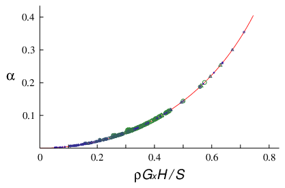
Steady solutions obtained by the time-dependent calculation during the forcing, approximately for $T_{*}/2<t<(3/4)T_{*}$, are checked against the analytical solution in Fig. 4. The curve shows $\max_{\zeta}{\alpha}$ given by Eq. (51) as a function of $\rho G_{x}H/S$. The symbols, consisting of 122 circles ($T_{*}=100\tau_{0}$) and 110 triangles ($T_{*}=200\tau_{0}$), indicate the numerical values of $\max_{\zeta}{\alpha}$ calculated within the range $\sigma_{\text{Y}}<\rho G_{x}H<0.72\,S$, $0.05\,S\leq\sigma_{\text{Y}}\leq 0.30\,S$, and $0.20\,\ell_{0}\leq H\leq 8.0\,\ell_{0}$. The size (and the color) of each symbol indicates the magnitude of $\sigma_{\text{Y}}/S$. Fig. 4 demonstrates that the value of steady $\alpha$ is independent of $\sigma_{\text{Y}}$, once $\rho G_{x}H$ exceeds it. For $T_{*}=100\tau_{0}$, there were several cases for which $\alpha$ did not attain its steady value (with the criterion $\Delta{\alpha}/|\alpha|=0.02$); these cases are eliminated from Fig. 4 for clarity. Such exceptional cases did not occur for $T_{*}=200\tau_{0}$.

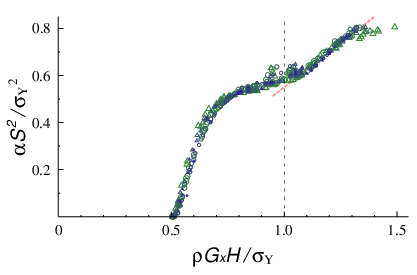
As an explanation of the Nakahara effect, it is essential to show that some of $\alpha$ remains in the paste even after the flow is stopped, instead of decaying away. Fig. 5 shows the numerical values of $\max_{\zeta}{\alpha}$ remaining steady (not to decay any more) after the flow is stopped. Here not $\alpha$ itself, but $\alpha S^{2}/\sigma_{\text{Y}}^{2}$ is plotted against $\rho G_{x}H/\sigma_{\text{Y}}$ for $\rho G_{x}H>\sigma_{\text{Y}}/2$ (the ranges of $\sigma_{\text{Y}}/S$ is the same as in Fig. 4, and that of $H/\ell_{0}$ is $0.05\,\ell_{0}\leq H\leq 8.0\,\ell_{0}$). The values of residual $\alpha$ for $\sigma_{\text{Y}}<\rho G_{x}H<1.3\,\sigma_{\text{Y}}$ is fitted by

In contrast to the steady value of $\alpha$ in the flow subject to the driving force, the residual value of $\alpha$ in Eq. (53) is strongly dependent on $\sigma_{\text{Y}}$. In particular, if $\rho G_{x}H/\sigma_{\text{Y}}$ is kept constant, Eq. (53) states that the residual value of $\alpha$ is scaled by $(\sigma_{\text{Y}}/S)^{2}$. This result seems understandable if we assume that, during the decay of $\alpha$ and $\tilde{\sigma}={\sigma_{xz}}/S$, the first equal sign in Eq. (50) remains valid, until $\sigma_{xz}$ reaches the threshold value $\sigma_{\text{Y}}$. This gives a rough estimation of the residual $\alpha\simeq 0.5\,(\sigma_{\text{Y}}/S)^{2}$. Unfortunately, theoretical clarification of Eq. (53) in regard to its dependence on $\rho G_{x}H/\sigma_{\text{Y}}$ is not currently available.

References

- [1] M. C. Miguel and M. Rubi, Jamming, Yielding, and Irreversible Deformation in Condensed Matter (Springer-Verlag, 2006), ISBN 3540300287.
- [2] A. Nakahara and Y. Matsuo, Bussei Kenkyû (Kyoto) 81, 184 (2003), (in Japanese).
- [3] A. Nakahara and Y. Matsuo, J. Phys. Soc. Japan 74, 1362 (2005), eprint cond-mat/0501447v2.
- [4] A. Nakahara and Y. Matsuo, J. Stat. Mech. (2006a), P07016.
- [5] A. Nakahara and Y. Matsuo, Phys. Rev. E 74, 045102(R) (2006b).
- [6] H. Kawazoe, K. Kanemura, and Ooshida Takeshi, (under preparation).
- [7] L. D. Landau and E. M. Lifshitz, Fluid Mechanics, vol. 6 of Theoretical Physics (Butterworth-Heinemann, 1987).
- [8] H. Schlichting and K. Gersten, Boundary Layer Theory (Springer-Verlag, 2000), 8th ed., ISBN 3-540-66270-7.
- [9] D. D. Joseph, Fluid Dynamics of Viscoelastic Liquids (Springer-Verlag, 1990).
- [10] Y. Miyamoto, K. Fukao, H. Yamao, and K. Sekimoto, Phys. Rev. Letter 88, 225504 (2002), eprint cond-mat/0111005.
- [11] K. Kruse, J. F. Joanny, F. Jülicher, J. Prost, and K. Sekimoto, Phys. Rev. Letter 92, 078101 (2004).
- [12] K. Kruse, J. F. Joanny, F. Jülicher, J. Prost, and K. Sekimoto, Eur. Phys. J. E 16, 5 (2005).
- [13] Ooshida Takeshi and K. Sekimoto, Phys. Rev. Letter 95, 108301 (2005).
- [14] R. Hill, The Mathematical Theory of Plasticity (Oxford University Press, 1950).
- [15] H. Hencky, Zeits. Ang. Math. Mech. 4, 323 (1924).
- [16] A. Bennett, Lagrangian fluid dynamics (Cambridge University Press, 2006), ISBN 0-521-85310-9.
- [17] J. E. Marsden and T. J. Hughes, Mathematical Foundations of Elasticity (Dover Publications, 1994), ISBN 0-486-67865-2, publised originally by Prentice-Hall, 1983.
- [18] M. Nakahara, Geometry, Topology, And Physics (Institute of Physics Publishing, 1990), ISBN 0-85274-095-6.
- [19] E. H. Lee, ASME J. Appl. Mech. 36, 1 (1969).
- [20] V. A. Lubarda and E. H. Lee, ASME J. Appl. Mech. 48, 35 (1981).
- [21] E. C. Bingham, Fluidity and plasticity (McGraw-Hill, New York, 1922).
- [22] C. C. Mei and M. Yuhi, J. Fluid Mech. 431, 135 (2001).
- [23] J. Duran, Sands, Powders, and Grains; An Introduction to the Physics of Granular Materials (Springer-Verlag, New York, 2000), ISBN 0-387-98656-1, translated by Axel Reisinger.
- [24] W. H. Press, B. P. Flannery, S. A. Teukolsky, and W. T. Vetterling, Numerical Recipes in C (Cambridge University Press, 1988).
- [25] I. S. Aranson and L. S. Tsimring, Reviews of Modern Physics 78, 641 (2006).
- [26] K. Sekimoto, J. Non-Newtonian Fluid Mech. 46, 219 (1993).
- [27] J. M. Carlson and A. A. Batista, Phys. Rev. E 53, 4153 (1996).
- [28] R. M. Nedderman, Statics and Kinematics of Granular Materials (Cambridge University Press, 1992), ISBN 978-0521404358.
- [29] K. Kamrin and M. Z. Bazant, Phys. Rev. E 75, 041301 (2007).
- [30] K. Sekimoto, J. Non-Newtonian Fluid Mech. 39, 107 (1991).
- [31] T. Ohzono and M. Shimomura, Phys. Rev. E 72, 025203(R) (2005).
- [32] L. D. Landau and E. M. Lifshitz, Theory of Elasticity, vol. 7 of Theoretical Physics (1986).
- [33] P. M. Chaikin and T. C. Lubensky, Principles of condensed matter physics (Cambridge University Press, 1995).
- [34] D. McLean, Mechanical properties of metals (Wiley, 1962).
- [35] K. Miyazaki and D. R. Reichman, Phys. Rev. E 66, 050501(R) (2002).
- [36] M. Fuchs and M. E. Cates, Phys. Rev. Letter 89, 248304 (2002).
- [37] M. Otsuki and S. Sasa, J. Stat. Mech. (2006), L10004.
- [38] U. Frisch, Turbulence: the legacy of A.N. Kolmogorov (Cambridge University Press, 1995), ISBN 0521457130.
- [39] R. H. Kraichnan, Physics of Fluids 8, 575 (1965).
- [40] Y. Kaneda, J. Fluid Mech. 107, 131 (1981).
- [41] S. Kida and S. Goto, J. Fluid Mech. 345, 307 (1997).
- [42] M. Otsuki, Phys. Rev. E 72, 046115 (2005).
- [43] V. Ya. Shkadov, Izv. Akad. Nauk. SSSR, Mekh. Zhid. i Gaza 1, 43 (1967).
- [44] C. Ruyer-Quil and P. Manneville, Eur. Phys. J. B 6, 277 (1998).
- [45] H.-C. Chang and E. Demekhin, Complex Wave Dynamics on Thin Films (Elsevier, 2002).
- [46] A. J. C. de Saint-Venant, C. R. Acad. Sci. Paris 73, 147 (1871).
- [47] Y. Forterre and O. Pouliquen, J. Fluid Mech. 486, 21 (2003).
- [48] R. B. Bird, R. C. Armstrong, and O. Hassager, Dynamics of polymeric liquids, vol. 1 (Wiley, 1987), 2nd ed., ISBN 047180245X.