Double heavy-quarkonium production from electron-positron annihilation in the Bethe-Salpeter formalism

It is well known that there is a significant discrepancy between the experimental measurements [1, 2] and the NRQCD predictions [3, 4] for the process $e^{+}e^{-}\to J/\psi\,\eta_{c}$ at energy $\sqrt{s}\approx 10.6$ GeV. To reduce the discrepancy many efforts have been made. For example, as discussed in Ref. [5], corrections from pure electromagnetic interactions are introduced into the non-relativistic QCD (NRQCD) factorization formalism; the next-to-leading-order contributions of strong interaction are taken into account in Refs. [6, 7]; in Ref. [8], the authors take into account corrections to the $J/\psi$ leptonic decay width and the scale dependence of the leading-order prediction; etc.

Indeed, NRQCD should work well while dealing with the processes where heavy flavors are involved, especially in this concerned reaction where only heavy flavors exist. In the scenario of NRQCD an expansion is carried out with respect to powers of the relative three-velocity $v$ which reflects the relativistic effects. Even though, in this reaction, the relativistic effects obviously are smaller than in the processes dominated by light flavors, they still may cause sizable contributions. Later works confirm this viewpoint. One needs, therefore, to incorporate the relativistic corrections into the theoretical calculations in an appropriate way. There are various ways to take into account the relativistic corrections. Ebert et al. carefully studied the corrections from relativistic effects [9] and indicated that with the relativistic effects being properly handled, a prediction for the cross section which is consistent with the present experimental measurement can be obtained.

Moreover, the factorization scheme should work in this case, because the production of $J/\psi+\eta_{c}$ from $e^{+}e^{-}$ via electromagnetic interaction can be regarded as a reversed Drell-Yan process where the factorization is proved. Thus one can factorize the hard and soft processes and then a convolution integration over the two parts results in the final amplitude. Therefore, one only needs to consider the relativistic corrections appearing in the soft part, i.e. in the hadronization process because the hard part is carried out in the framework of quantum field theory which is completely in the relativistic covariant form.

To understand the experimental results, many authors have proposed various projects to improve the theoretical framework in addition to NRQCD. For example, this problem was discussed with the method of perturbative QCD (pQCD) . In Ref. [10], the corrections of higher-twist wave functions were included in pQCD and the light-front quark model.

Discussions given in Refs. [6, 7, 11, 12] suggest that to reduce the large discrepancy between the experimental results and the theoretical predictions based on NRQCD for the exclusive process with the final state which is composed of two charmonia, large next-to-leading-order (NLO) corrections may appear (the ‘NLO’ contribution is about 1.8 to 2.1 times of the leading-order one). Including this large NLO contributions, their results are close to the lower bound set by the Babar and Belle collaborations for the double-charmonia production. The authors also indicate that including the relativistic corrections can further enhance the estimated value.

We would rather incline to believe that because of the validity of the factorization, perturbative calculation is suitable and, therefore, in our calculation we will ignore the contribution of the next-to-leading order corrections. Then one should expect that a larger correction may come from the soft part, i.e. the relativistic effect may be significant.

As mentioned before, Ebert et al. considered such effects [9]. Alternatively, in this work, for properly incorporating relativistic effects, we try to evaluate this exclusive process in the Bethe-Salpeter (BS) formalism [13]. The BS equation is in principle established in the framework of relativistic quantum field theory, therefore, it is supposed to include all relativistic effects. Of course, to solve this equation in practice, one needs to adopt some approximations such as the instantaneous approximation where part of the relativistic effects are lost. However, in many cases, such loss is not serious. Indeed, the BS formalism is suitable for studying the binding systems composed of two heavy charm and anti-charm quarks (or bottom flavors). The transition amplitudes can be obtained, in a natural way, to be an overlap integration of BS wave functions (see e.g. Ref. [14]). In order to simplify the calculation, we will further impose the heavy quark limit [15, 16, 17], i.e. all the $1/m_{Q}$ corrections are neglected in the calculation in this paper. Under this limit, our result shows that, at the leading order of $\alpha_{s}$, the theoretical prediction is comparable with the experimental result [1, 2]. We attribute this mainly to the inclusion of relativistic effects in our formalism. We will come back to give more discussion on this point in the last section.

The remainder of this paper is organized as follows. In Sec. II, we will study the BS equations for the vector and pseudo-scalar quarkoniums. In Sec. III, we will calculate the cross section of the process $e^{+}e^{-}\to J/\psi\,\eta_{c}$ in the BS formalism. In this section, we will also give the prediction for the much smaller cross section of the exclusive process with double bottomonium production, $e^{+}e^{-}\to\Upsilon(1S)\eta_{b}$. Sec. IV is reserved for our conclusions and discussions.

The BS wave function for a meson which is composed of a quark and an anti-quark is defined as

where $P$ is the momentum of the meson, $\psi_{\alpha}^{i}(x_{1})$ and $\overline{\psi}_{\beta}^{j}(x_{2})$ are the field operators of the quark and anti-quark, respectively, $\alpha,\beta$ are Dirac spinor indices, and $i,j$ denote the color indices. In momentum space the BS equation for the wave function $\chi_{{}_{P}}^{\,}(x_{1},x_{2})_{\alpha\beta}$ can be written as (see Refs. [18, 19] for example)

where $p,k$ represent the relative momenta between the quark and anti-quark, $m_{1}(p_{1})$ and $m_{2}(p_{2})$ are the masses (momenta) of the quark and anti-quark, respectively, and $V_{P}(p,k)$ is the kernel. The spinor indices are suppressed for simplicity. For the heavy quarkonium $Q\overline{Q}$ ($Q=c,b$) studied in this paper, we have $m_{1}=m_{2}=m_{Q}$ and then $p_{1}=P/2+p$ and $p_{2}=-P/2+p$.

To simplify the calculation we will take the heavy quark limit throughout this paper. In this limit, the propagators of the heavy quark and heavy anti-quark ($S(p_{1})$ and $S(p_{2})$, respectively) can be simplified in the following way [20]:

where we have defined the binding energy $E_{0}=M-2m_{Q}$, $v=P/M$ is the ‘four-velocity’ of the meson, $M$ is the mass of the meson and $p_{\!{}_{\ell}}=v\cdot p$. With this simplification, the BS equation (2) becomes

From this expression, one can easily see that the BS wave function $\chi_{{}_{P}}^{\,}$ satisfies ${\not\!v}\chi_{{}_{P}}^{\,}=\chi_{{}_{P}}^{\,}$ and $\chi_{{}_{P}}^{\,}{\not\!v}=-\chi_{{}_{P}}^{\,}$. Then, in the heavy quark limit, similar to the case for the diquark system studied in Ref. [21], we have the following very simple parameterizations for the BS wave functions of vector and pseudoscalar $Q\overline{Q}$ mesons (which are denoted by the subscripts ”$a$” and ”$b$”, respectively):

where $\varepsilon^{(s)}$ is the polarization vector of the vector quarkonium which is orthogonal to the velocity, $\varepsilon^{(s)}\cdot v=0$, $f_{a}$ and $f_{b}$ are scalar functions of the relative momentum $p$.

In this work, following the standard procedure for solving the BS equation we impose the instantaneous approximation onto the kernel as $V_{P}(p,k)=V({\bf p},{\bf k})$. Taking the concrete steps given in Ref. [18], we can obtain this kernel by a Fourier transformation of the Cornell potential which contains a linear piece and a Coulomb-type piece, $-iV(r)=I\otimes IV_{s}(r)+\gamma^{\mu}\otimes\gamma_{\mu}\,V_{v}(r)$, where $V_{s}(r)=\lambda r+V_{0}$ and $V_{v}(r)=-\frac{4}{3}\frac{\alpha_{s}}{r}$. To avoid any infrared divergence, a convergent factor $e^{-\beta r}$ is introduced into the potential,

After the Fourier transformation, the kernel in momentum space reads [18]: $-iV({\bf q})=I\otimes IV_{s}({\bf q})+\gamma^{\mu}\otimes\gamma_{\mu}\,V_{v}({\bf q})$, where

and the effective coupling constant is given by $\alpha_{s}({\bf q})=4\pi/9\log{(a+\frac{{\bf q}^{2}}{\Lambda^{2}_{QCD}})}$ with $a$ being a parameter which freezes the running coupling constant at low energy.

With this kernel, the BS equation (5) is written as

where ${\bf q}={\bf p}-{\bf k}$. Substituting the BS wave functions (6) and (7) into Eq. (10) we get the following component equations for vector and pseudo-scalar quarkonia:

For later convenience, here we also write out the BS equation for the conjugate wave function,

To solve the BS equation (11), for convenience, we can choose a coordinate frame in which the binding system is static. The BS wave functions in this frame are given in Eqs. (6) (7), where $f_{a}(p)$ and $f_{b}(p)$ are Lorentz scalar functions. Then the longitudinal component $p_{\!{}_{\ell}}=p^{0}$. After carrying out the integrations over $p^{0}$ and $k^{0}$ on both sides of the BS equation along some proper contour, Eq. (11) becomes ¹¹ 1 In pratical calculation, to obtain the reasonable BS wave functions, we will replace $E_{0}$ by $M_{a(b)}-2\sqrt{{\bf k}^{2}+m_{Q}^{2}}$ in the following BS equation. This replacement is equivalent to regaining some part of $1/m_{Q}$ effects in the calculation.

where we have defined the instantaneous wave functions by $\widetilde{f}_{a(b)}({\bf p})=\int{dp^{0}\over 2\pi}f_{a(b)}(p)$.

Now we turn to discuss the exclusive process in the electron-positron collisions with the final state of two heavy quarkonia. The relevant Feynman diagrams for the process $e^{+}e^{-}\to J/\psi\,\eta_{c}$ are depicted in Fig. 1.

Since the s-channel gluon turns into $c\bar{c}$ in this process, hence the gluon is hard and the energy scale for this process is large. Therefore, the perturbative calculation in QCD to lowest order of $\alpha_{s}$ expansion is expected to be sufficient. We will not consider the contributions from diagrams of higher-order in $\alpha_{s}$. Furthermore, we do not consider any higher order corrections from the pure electromagnetic interactions, which should be small and were discussed in Ref. [5].

One of the amplitudes in Fig.1 can be written as

where $C=4/3$ is the color factor, $\sqrt{s}$ is the total energy in the center-of-mass frame, and $e_{Q}$ is the electric charge of the quark $Q$. The conjugation of the BS wave function is defined by $\overline{\chi}_{{}_{P}}^{\,}\equiv\gamma^{0}(\chi_{{}_{P}}^{\,})^{\dagger}\gamma^{0}$. The momenta of the quark and anti-quark within the final state are $q^{\prime}_{1}=\frac{1}{2}P_{a}+q_{a}$ , $q_{3}=\frac{1}{2}P_{a}-q_{a}$ , $q_{4}=\frac{1}{2}P_{b}+q_{b}$ , $q_{2}=\frac{1}{2}P_{b}-q_{b}$ , and the momenta in the gluon and the quark propagators are given by

respectively. Since an integration is needed to obtain the amplitude (19) and since the propagators of the quark and the gluon depend on the relative momenta $q_{a}$ and $q_{b}$ one can expect that the calculation is very complicated. To simplify the calculation, we assume that the propagators of the quark and the gluon are independent of relative momenta $q_{a}$ and $q_{b}$ (see, e.g. Ref. [21]). This simplification is appropriate since the masses of heavy quarks are large compared with the relative momenta, which are of order $\alpha_{s}m_{Q}$. Then the momenta $q_{1}$ and $k$ of the propagators are large compared with the relative momenta $q_{a}$ and $q_{b}$. One may expect that, in the heavy quark limit, the calculation without taking into account the relative momenta should be exact. ²² 2 The energy scale $\mu$ is of the same order of $m_{Q}$ and then, in the heavy quark limit, $\alpha_{s}(\mu)\sim 1/\log(m_{Q}/\Lambda_{\rm QCD})\to 0$.

With the above approximation in mind, the momenta $k$ and $q_{1}$ can be written as: $k\approx(P_{a}+P_{b})/2$, $q_{1}\approx P_{a}+P_{b}/2$ which lead to $k^{2}\approx s/4$, $q_{1}^{2}\approx s/2+M_{a}^{2}/2-M_{b}^{2}/4\approx s/2+m_{c}^{2}$. Furthermore, we will make use of the approximation $M_{J/\psi}\approx M_{\eta_{c}}\approx 2m_{c}$ in the calculation throughout this paper. Then the amplitude (19) can be written as

From the component expressions of the BS wave functions (6) and (7), we can see $\overline{\chi}_{{}_{P_{a}}}^{\,(s)}={\not\!\varepsilon}^{(s)}(1+{\not\!v_{a}})M_{a}f_{a}$ and $\overline{\chi}_{{}_{P_{b}}}^{\,}=\gamma_{5}(1+{\not\!v_{b}})M_{b}f_{b}$. ³³ 3 We have rotated the phase of the wave function to make $f_{a}$ and $f_{b}$ be real. Substituting the BS wave functions into the trace in the above amplitude, one achieves

where $\alpha_{s}=g_{s}^{2}/4\pi$, $\alpha_{\rm em}=e^{2}/4\pi$, $\psi_{a}$ and $\psi_{b}$ are two numbers defined by the integrations over $f_{a}$ and $f_{b}$, respectively,

The total amplitude for the process $e^{+}e^{-}\to J/\psi\,\eta_{c}$ can be obtained by summing over all the amplitudes of the diagrams shown in Fig. 1.

The unpolarized total cross section (see e.g. Ref. [22]) is obtained by summing over various $J/\psi$ spin-states and averaging over those of the initial state $e^{+}e^{-}$,

where the masses of the electron and positron are ignored in the calculation. The explicit expression for the total amplitude $|\mathcal{M}_{\rm total}|^{2}$, which is the sum of all diagrams shown in Fig. 1, is written as

where $t=(p_{1}-P_{a})^{2}$ and $u=(p_{1}-P_{b})^{2}$ are the Mandelstam’s variables.

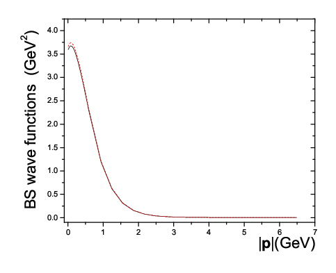
Then we have

Consequently, the total cross section is obtained as

If we vary $m_{c}$ and $\alpha_{s}$ within $10\%$ we can get an errors $\pm 1.6fb$.

In this paper, we study the exclusive processes of $e^{+}e^{-}$ annihilating into two quarkonia in terms of the BS formalism. We find that, in the heavy quark limit, the cross section is $\sigma[e^{+}e^{-}\to J/\psi\,\eta_{c}]=22.3$ fb, which is compatible with the Babar’s data, $\sigma[e^{+}e^{-}\to J/\psi\,\eta_{c}]\geq 17.6\pm 2.8\pm 2.1$ fb [2], and the Belle’s data, $\sigma[e^{+}e^{-}\to J/\psi\,\eta_{c}]\geq 25.6\pm 2.8\pm 3.4$ fb [1]. Because the BS formalism is established based on the relativistic quantum field theory, one has a strong reason to believe that some (perhaps not all) relativistic effects are automatically included in the calculations. The missing part may come from the instantaneous approximation which is necessary for solving the BS equation. Since the approximation is proved to be reasonable in theoretical calculations for other similar processes, we may be convinced that the missing part is not significant. Thus we expect that the non-leading-order contributions, from extra $1/m_{Q}$ which is indeed a relativistic effect, and $\alpha_{s}$ corrections, should be small. Our result is different from those given in Refs. [6, 7, 11, 12] in the NRQCD framework, where the leading-order contribution is too small to be comparable with the experimental data. In order to reduce the discrepancy between the experimental data and the theoretical predictions based on NRQCD, large non-leading-order contributions (including $\alpha_{s}$ or/and relativistic correction(s)) are required in the NRQCD framework and the value of the total non-leading-order correction is nearly twice of the leading-order one.

We also calculate the cross section for the exclusive process with two bottomonia as the final state, $\sigma[e^{+}e^{-}\to\Upsilon(1S)\eta_{b}]=(0.16\,\hbox{-}\,0.06)$ fb corresponding to the range of the total energy $\sqrt{s}=(25\,\hbox{-}\,30)$ GeV. Since $m_{b}\gg m_{c}$, the non-leading-order contributions, including effects of higher orders in $1/m_{b}$ and $\alpha_{s}(2m_{b})$ expansions, should be much smaller than those in the charmonium case. Therefore, we expect that the calculation in the bottomonium case is much more precise than that in the charmonium case. Even though such processes cannot be measured at present due to the constraint of the available energy range at the B-factories, the planned ILC will be a powerful facility to testify this result.

Due to the obvious advantage of the BS formalism for dealing with the processes where heavy flavors are involved, we may hope that the obtained results are close to reality.

It will be interesting to study the non-leading-order contributions in the formalism used in this paper and check whether our expectation about the non-leading-order contributions is right. This task is beyond the scope of this paper and will be discussed elsewhere.