EFFICIENT SPACETIME MESHING WITH NONLOCAL CONE CONSTRAINTS
Abstract
Spacetime Discontinuous Galerkin (DG) methods are used to solve hyperbolic PDEs describing wavelike physical phenomena. When the PDEs are nonlinear, the speed of propagation of the phenomena, called the wavespeed, at any point in the spacetime domain is computed as part of the solution. We give an advancing front algorithm to construct a simplicial mesh of the spacetime domain suitable for DG solutions. Given a simplicial mesh of a bounded linear or planar space domain , we incrementally construct a mesh of the spacetime domain such that the solution can be computed in constant time per element. We add a patch of spacetime elements to the mesh at every step. The boundary of every patch is causal which means that the elements in the patch can be solved immediately and that the patches in the mesh are partially ordered by dependence. The elements in a single patch are coupled because they share implicit faces; however, the number of elements in each patch is bounded. The main contribution of this paper is sufficient constraints on the progress in time made by the algorithm at each step which guarantee that a new patch with causal boundary can be added to the mesh at every step even when the wavespeed is increasing discontinuously. Our algorithm adapts to the local gradation of the space mesh as well as the wavespeed that most constrains progress at each step. Previous algorithms have been restricted at each step by the maximum wavespeed throughout the entire spacetime domain.
ABSTRACT
Keywords: mesh generation, unstructured meshes, advancing front, partial differential equations, discontinuous Galerkin, nonlinear hyperbolic PDE
1 Introduction
Simulation problems in mechanics consider the behavior of an object or region of space over time. Scientists and engineers use conservation laws and hyperbolic partial differential equations (PDEs) to model transient, wavelike phenomena propagating over time through the domain of interest. Example applications are numerous, including, for instance, the equations of elastodynamics in seismic analysis and the Euler equations for compressible gas dynamics. Closed-form solutions are typically unavailable for these problems, so analysts usually resort to numerical approximations.
Finite element methods (FEM) are popular options for solving this class of problems. In the standard semi-discrete approach, a finite element mesh discretizes space to generate a system of ordinary differential equations in time that is then solved by a time-marching integration scheme. Most semi-discrete methods impose a uniform time step size over the entire spatial domain, i.e., the time step does not adapt to the local gradation of the space mesh. Therefore, the resulting spacetime mesh consists of many more elements than required by physical causality. Hence, algorithms that use a nonuniform time step size can substantially improve computational efficiency.
Spacetime discontinuous Galerkin (DG) methods have been proposed by Richter [8], Lowrie et al. [7], and Yin et al. [11] for solving systems of nonlinear hyperbolic partial differential equations. Like traditional finite element methods, spacetime DG methods use basis polynomials to approximate the solution within each element; however, unlike traditional FEM methods, these basis polynomials have local support restricted to each element and the basis polynomials of adjacent elements do not have to agree on their common intersection. This approach eliminates artificial coupling between adjacent elements when the mesh satisfies certain causality constraints. (For further background on general discontinuous Galerkin methods, we refer the reader to Cockburn, Karniadakis, and Shu [3].)
Üngör and Sheffer [10] and Erickson et al. [4] developed the first algorithm, called ‘TentPitcher’, to build graded spacetime meshes over arbitrary simplicially meshed spatial domains, suitable for spacetime DG solutions. Unlike most traditional approaches, the TentPitcher algorithm does not impose a fixed global time step on the mesh, or even a local time step on small regions of the mesh. Rather, it produces a fully unstructured simplicial spacetime mesh, where the duration of each spacetime element depends on the local feature size and quality of the underlying space mesh.
Efficient spacetime meshing relies on the notion of the domain of influence and the domain of dependence of an event. Imagine dropping a pebble into a pond—circular waves propagate outwards from the point of impact. The frontier of expanding waves sweeps out a cone in spacetime called the domain of influence of the event. The radius of the domain of influence at any time is the radius of the circular disc consisting of all points on the surface where the initial wave has arrived. The domains of influence and dependence can be approximated by right circular cones with common apex (Figure 1). The symmetric double cone representing the domains of influence and dependence at points in spacetime can be described by a scalar field where , the wavespeed at , specifies how quickly the radius of domains of influence and dependence of grows as a function of time. Smaller values of , i.e., steeper cones, correspond to slower wavespeeds. The wavespeed at a point in spacetime is, in general, part of the solution of the PDE at that point. The slope of the cones of influence and dependence of , denoted by , is the reciprocal of the wavespeed—larger slopes mean steeper cones and therefore slower wavespeeds, and smaller slopes mean shallower cones and faster wavespeeds.
Given a simplicial mesh of some bounded domain , the Tent Pitcher algorithm incrementally constructs a simplicial mesh of the spacetime domain using an advancing front method. The spacetime domain is the subset , a subset of Euclidean space one dimension higher. The algorithm progresses by adding simplices to the evolving mesh in small patches by moving a vertex of the front forward in time. The inflow and outflow boundaries of each patch (Figure 2) are causal by construction, i.e., each boundary facet separates the cone of influence from the cone of dependence of any point on (Figure 1). Equivalently, for every point on we have . If the outflow boundaries of a patch are causal, every point in the patch depends only on other points in the patch or points of inflow elements adjacent to the inflow boundaries of the patch. Therefore, the solution within the patch can be computed as soon as the patch is created, given only the inflow data from adjacent inflow elements. The elements within a patch are causally dependent on each other and must be solved as a coupled system. Provided the space mesh has constant degree, each patch contains only a constant number of elements and can therefore be solved in constant time. Therefore, the computation time required to compute the numerical solution is linear in the number of spacetime elements. Patches with no causal relationship can be solved independently. To minimize undesirable numerical dissipation and the number of patches, we would like the boundary facets of each patch to be as close as possible to the causality constraint without violating it.
The causality constraint limits the progress in time at each step, i.e., the height of each tentpole is constrained. For spatial domains of dimension , it is not trivial to guarantee that the advancing front algorithm can always make progress. We require that for any target time value the algorithm will compute a mesh of the spacetime volume and the solution everywhere in this volume in finitely many steps. The target time is not known a priori because it depends on the evolving physics. The original Tent Pitcher algorithm proposed by Üngör and Sheffer [10] applied to one- and two-dimensional space domains. The algorithm could guarantee progress only if the input triangulation contained only angles less than 90 degrees and if the wavespeed did not increase or increased smoothly. Erickson et al. [4] extended Tent Pitcher to arbitrary spatial domains in any dimensions by imposing additional constraints, called progress constraints. The progress constraint applied to a single simplex on the front limits the amount of progress in time when some vertex of the simplex is pitched. The progress constraint is a function of the shape of the simplex. The geometric constraints that limit the height of each tentpole are called cone constraints.
All the results so far have applied to the case where the wavespeed at a given point is either constant, decreasing, or increasing smoothly as a Lipschitz function. (See Alper Üngör’s PhD thesis [9] for the details.) When the wavespeed changes, the previous algorithms take the fastest that the wavespeed can ever be and use that as a conservative upper bound on the wavespeed at any time. One would like an algorithm that adapts to increasing wavespeeds so that fewer spacetime elements, and therefore less computation time, are required to mesh a given volume.
In this paper, we give an advancing front algorithm to construct a spacetime mesh over an arbitrary linear or planar space mesh (). Our algorithm extends TentPitcher to the case when the wavespeed can be an arbitrary scalar field over the spacetime domain. In particular, our algorithm guarantees finite positive progress at each step even when the wavespeed at a given point increases discontinuously and unpredictably over time.
The main contributions of this paper are twofold. We give a novel characterization of fronts that are always guaranteed to progress, which we call progressive fronts, and give a lower bound on the progress guarantee at each step which depends only on the local size of the mesh and the wavespeed that most constrains the duration of the current patch. The minimum progress guarantee at any step is a positive quantity bounded away from zero, so the front is guaranteed to progress past any target time in a finite number of steps. The second contribution of this paper is to give geometric constraints on the front at any step that guarantee that the front can progress in the next step and so on inductively at every step. The geometric constraints are simple to express and to compute. Intuitively, the geometric constraints that apply at any given iteration of the algorithm are predicted by looking ahead at the next iteration of the algorithm. We also give an efficient algorithm to maximize the progress at every step subject to these constraints. The novelty of our characterization of progressive fronts and of our algorithm is that we resolve the following conundrum. The progress of the front at each step is limited by the progress constraint that must be satisfied by the next front at step . However, we do not know what is the next front unless we know how much progress is possible at step .
The paper by Erickson et al. [4] contains an error in the statement of the causality constraint when obtuse triangles are involved; therefore, their proof of correctness is incomplete because it omits the obtuse angle case. While their proof can be fixed, we prefer our new algorithm, which is provably correct even when the wavespeed is constant or does not increase. Our new progress constraints are potentially weaker than those of Erickson et al. [4].
Our algorithm is the first algorithm to build spacetime meshes over arbitrary planar triangulated spatial domains suitable for solving nonlinear hyperbolic PDEs, where the wavespeed at any point in spacetime depends on the solution and cannot be computed in advance. Moreover, the solution can change discontinuously, for instance when a shock propagates through the domain.

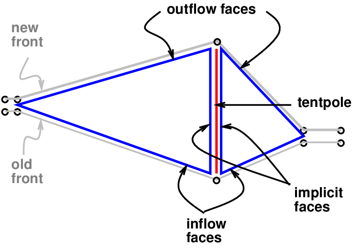
The input to our advancing front algorithm is a simplicially meshed bounded domain where and the initial conditions of a nonlinear hyperbolic PDE. The space mesh describes the situation at time equal to zero, specifically, the slope at every point in at time zero. We allow more general initial conditions but we will postpone a description of those conditions until later sections. Our meshing algorithm is an advancing front procedure which alternately constructs a new patch of elements and invokes a spacetime DG finite element method to compute the solution within that patch. At every iteration, the front is the graph of a continuous piecewise linear time function . The front is linear within every simplex of and for every point . The front is a terrain whose facets correspond to simplices in the underlying space mesh. Each facet of the front coincides with the outflow face of a patch in the past and the inflow face of a patch in the future. We say that a front is causal if every simplex of the front is causal. To advance the front , the algorithm chooses an arbitrary vertex from the front and lifts it to a new point where and for every other vertex we have . The spacetime volume between the new front and the old front is called a tent. The tent is meshed with simplices sharing the edge called the tentpole. The height of the tentpole is the duration . Consider a planar space mesh . For each triangle incident on , the tetrahedron belongs to the patch. The outflow face and the inflow face are causal boundaries. The triangles and are implicit faces. Since the implicit faces are vertical they are not causal boundaries and so elements within the patch are coupled. The elements below the front whose outflow faces intersect any of the inflow faces of the new patch are inflow elements. We pass the newly constructed patch along with all its inflow elements to a DG solver. The DG solver returns as part of the solution the slope at every point on every outflow face of the patch. The new front and the output of the DG solver are the input to the next iteration of the algorithm.
Since we are interested in causal fronts only, henceforth it is implicit that every front considered is causal.
We assume that the slope at any point is bounded by the minimum and the maximum slopes anywhere in the cone of dependence of . Hence, given a front and a point in the future, the slope at is no smaller than the slope at for every point on the front such that is in the cone of influence of .
It can be computationally very expensive to determine the shallowest cone of influence that contains a given point . In particular, the shallowest cone of influence containing may correspond to a nonlocal point , one arbitrarily distant from . To compute this nonlocal cone constraint efficiently, we use a standard hierarchical decomposition, called a bounding cone hierarchy, of the space domain. The elements in the hierarchy correspond to subsets of the space domain. For each element of the hierarchy, we compute the minimum slope within the corresponding subset of the space domain. The smallest element in the hierarchy is a single simplex. In order to determine the strictest cone constraint that applies locally, we traverse the hierarchy until we determine the simplex with minimum slope whose cone of influence contains . In practice, we expect that our algorithm has to examine only a small subset of the hierarchy. In the worst case, the algorithm has to examine every simplex of the front but in that case the algorithm will be at most a constant factor slower than one that does not use a bounding cone hierarchy. When a patch is solved, the bounding cones are updated with the new slopes by traversing a path from a leaf to the root of the hierarchy. This hierarchical approximation technique has been applied very successfully to numerous simulation problems, such as the Barnes-Hut divide-and-conquer method [2] for -body simulations, as well as to collision detection in computer graphics and robot motion planning [6] and for indexing multi-dimensional data in geographic information systems [5].
1.1 Notation
We use lowercase letters like , , to denote points in space and uppercase letters like , , to denote points in spacetime. A front is a piecewise linear function . For a simplex (of any dimensions) of , let denote the time function restricted to and extended to the affine hull of ; in other words, is a linear function that coincides with for every point of . Let denote the front after the th step of the algorithm; is the initial front. For every , the front is a terrain whose facets are the simplices of . In other words, is a piecewise linear function such that for every simplex of , the functions and coincide at the vertices of .
For a time function we denote the gradient of by . A local minimum of the front is a vertex such that for every vertex that is a neighbor of . When the current front is clear from the context, for every point we use to denote the corresponding point on the front, i.e., .
For a point in spacetime, we use to denote the reciprocal of the wavespeed at . Let denote and denote . We assume that . For a simplex in spacetime, we use to denote the minimum of over all points in .
We say that a front is obtained by advancing a vertex of by if and for every other vertex we have . For any front , vertex , and real , let denote the front obtained from by advancing by .
1.2 Problem statement
The input to our problem is the initial front and the initial conditions of the PDE. We want an advancing front algorithm such that for every there exists a finite integer such that the front after the th iteration of the algorithm satisfies .
We say that a front is valid if there exists a positive real bounded away from zero such that for every there exists a sequence of fronts , , , , where , each front in the sequence obtained from the previous front by advancing some vertex by . What makes the definition of a valid front nontrivial is the requirement that all fronts be causal. The main difficulty in characterizing valid fronts arises when the wavespeed at a given point in the space domain increases discontinuously and unpredictably over time.
Our solution We define progressive fronts and prove that if a front is progressive then it is valid. We give an algorithm that given any progressive front constructs a next front such that is progressive. The volume between and is partitioned into simplices. The next front is obtained by lifting a local minimum of by a positive amount bounded away from zero. The algorithm can easily be parallelized to solve several patches asynchronously by lifting any independent set of vertices in parallel. Whenever the algorithm chooses to lift a local minimum, it is guaranteed to be able to lift it by at least which is a function of the input and bounded away from zero.
2 One-dimensional space domains
We begin by describing our algorithm to construct spacetime meshes over one-dimensional space domains. Even this simple case captures all but one aspect of the complexity of guaranteeing causality when wavespeeds are changing.
The space domain is a closed interval of the real line. The input space mesh is a subdivision of this interval into segments. Let denote the set of vertices of the space mesh . The initial front corresponds to for every vertex of the space mesh, but more generally, any (causal) front can be the initial front. Let denote the minimum length of any segment in the space mesh. Let denote the minimum slope over every point in the spacetime domain . Let denote .
In iteration of our advancing front algorithm (), we advance a single vertex , where is a local minimum of the current front , to get the new front , i.e., . More generally, we can advance any vertex or an independent set of vertices, not necessarily local minima, forward in time. The value of is bounded from above by the requirement that be causal.
Let be an arbitrary segment of the front . Without loss of generality, assume . Then, is causal if and only if the gradient of the time function restricted to is at most the slope , i.e., if and only if
| (1) |
Theorem 1.
Let be a front and let be an arbitrary local minimum of . Then, for every the front is causal.
Proof.
Only the segments of the front incident on advance along with . Consider an arbitrary segment incident on . Let and denote and respectively. We have because is a local minimum, , and . Therefore, the segment is causal. Since this is true of an arbitrary segment on the front , we have proved that that the front is causal. ∎
Theorem 2.
For any , if the front is causal then is valid.
Proof.
Consider step of the algorithm. By Theorem 1 the front such that is causal. Therefore, we have shown that if is causal then there is a front such that is causal. Note that . By induction on , and because is finite and is bounded, there exists a finite such that the front satisfies
for any real . Since is causal
Therefore, and so is valid. ∎
2.1 Being greedy at every step
 |
 |
 |
 |
 |
 |
 |
 |
 |
 |
 |
 |
 |
 |
 |
 |
We would like to maximize the progress at each step in a greedy fashion, i.e., given a front we would like to maximize where subject to the constraint that is causal. By Theorem 2, we can have . However, it may be possible to make further progress by setting higher, especially if each segment incident on each satisfies progress constraint [] for some at the end of the previous iteration.
For a fixed segment incident on let denote is causal where . To maximizing the progress at step , we would like to compute . The segment is causal if and only if the slope of is less than or equal to the slope of the cone of influence from every point on the front that intersects . A cone of influence intersects if and only if the cone intersects the tentpole . In general, a cone of influence from arbitrarily far away can intersect the tentpole at . See Figure 3. This is not the case when the wavespeed everywhere is the same. Therefore, in general, could be determined by a cone of influence of a point arbitrarily distant from .
Partition the front into two subsets of points: (i) points in the star of (“local” points), and (ii) points everywhere else on the front (“remote” points). Corresponding to each subset we have two disjoint subsets of cones of influence— and respectively. Each subset of cones limits the new time value of and so the final time value is the smaller of the two values for each of and taken separately.
Consider the subset . Let denote the smallest slope among all cones of influence in The segment is causal only if its slope is less than or equal to . Let be the maximum time value of for which the slope of is less than or equal to . The maximum exists because the set of feasible values is closed and therefore compact. To compute we substitute in the condition for causality of (Equation 1).
Next consider the subset . The front is strictly below every cone in because is causal. The segment is causal only if it is also strictly below every cone in . Given a cone , intersects if and only if intersects the tentpole . Let denote the smallest time value for which the tentpole where intersects exactly one cone in . The segment is causal only if . Note that the upper bound on imposed by remote cones is a strict inequality.
Therefore, the progress at step is limited because . To maximize the progress at the current step, we choose equal to minus the machine precision , or , whichever is larger.
Computing exactly
Computing is equivalent to answering a ray shooting query in the arrangement of the cones in . We use a bounding cone hierarchy obtained from a hierarchical decomposition of the space domain to efficiently answer the ray shooting query. The hierarchical decomposition of the space domain induces a corresponding hierarchical decomposition of every front. For each element of this hierarchy, we store a right circular cone that bounds the cone of influence of every point of the corresponding subset of the front. To answer the ray shooting query, we traverse the cone hierarchy from top to bottom starting at the root. At every stage, we store a subset of bounding cones such that every cone in is contained in some cone in the subset . The cones in are stored in a priority queue in non-decreasing order of the time value at which the vertical ray at intersects each cone. Initially, consists solely of the cone at the root of the hierarchy. At every stage, if the cone in that has the earliest intersection does not come from a leaf in the hierarchy then we replace it in the priority queue with its children. Continuing in this fashion, we eventually determine the single facet of the front such that the cone of influence from some point on this facet is intersected first by the vertical ray at . The time coordinate of the point of intersection is , the answer to the ray shooting query.
If the hierarchy is balanced its depth is where is the number of simplices in the space mesh. In 1DTime, we observed empirically that on average only a few nodes in the cone hierarchy were examined by this algorithm to determine the most constraining cone of influence.
Approximating
Since we know a range of values that contains , we can approximate up to any desired numerical accuracy by performing a binary search in this interval. At every iteration, we speculatively lift to the midpoint of the current search interval. Let be the speculative top of the tentpole at . We query the cones of influence in to determine the minimum slope among all cones that intersect . If the maximum slope of the outflow faces incident on is less than then we can continue searching in the top half of the current interval; otherwise, the binary search continues in the bottom half of the current interval. The search terminates when the search interval is smaller than our desired accuracy. A bounding cone hierarchy helps in the same manner as before to determine the minimum slope among all cones in that intersect .
Theorem 3.
Given a simplicial mesh of a bounded real interval where is the minimum length of a simplex of and is the minimum slope anywhere in our algorithm constructs a simplicial mesh of consisting of at most spacetime elements for every real .
Proof.
We have shown that every causal front in 1DTime is valid. In higher dimensions, additional progress constraints are necessary.
3 Planar space domains
In this section, we describe our algorithm for , i.e., for a triangulated planar space domain .
For planar domains, we encounter nontrivial progress constraints that are necessary to guarantee sufficient progress at each step, i.e., to guarantee that the height of the tentpole constructed at every step is positive and bounded away from zero. In the absence of such constraints, it was shown by Üngör and Sheffer [10], and by Erickson et al. [4] that if the space mesh contains an obtuse or a right triangle then Tent Pitcher will eventually construct a front such that no further progress is possible while maintaining causality. Erickson et al. [4] derived additional progress constraints that were sufficient to guarantee progress, even in the presence of obtuse angles, however only by assuming the minimum slope occurs everywhere in spacetime. In this section, we show how to relax these progress constraints so that they adapt to the slope of the most constraining cone of influence at every step. Our progress constraint is a function of the slope encountered locally in the next step of the algorithm, which may be substantially less constraining than the globally minimum slope.
Fix a real parameter . The space domain is a triangulation of a bounded subset of the plane . Let denote the minimum width of any triangle of the space mesh. Let denote the minimum over every point in the spacetime domain . Let denote .
Definition 1 (Progress constraint ).
Let be an arbitrary triangle of a front . Without loss of generality, assume . We say that the triangle satisfies progress constraint if and only if
where . Note that .
Suppose the lowest vertex is being advanced. As long as is the lowest vertex of , the progress constraint limits but is unchanged by lifting . When , the new lowest vertex is , so the progress constraint limits . (We can interpret the progress constraint inductively as a causality constraint on the -dimensional facet opposite where the relevant slope is .)
Definition 2 (Progressive).
Let be a front and let be a given triangle. Without loss of generality, assume . We say that the triangle is progressive if and only if both of the following conditions are satisfied by where for every :
- 1.
is causal, and
- 2.
satisfies progress constraint where .
We say that a front is progressive if every triangle on the front is progressive. Note that every progressive triangle or front is also causal.
3.1 A new advancing front algorithm
We are now ready to describe iteration of our advancing front algorithm for . Advance a single vertex by a positive amount, where is any local minimum of the current front , to get the new front such that for every triangle incident on the corresponding triangle on the new front is progressive. In the parallel setting, advance any independent set of local minima forward in time, each subject to the above constraint. The value of is constrained from above separately for each of the simplices incident on . The final value chosen by the algorithm must satisfy the constraints for each such triangle. Therefore, it is sufficient to consider each triangle incident on separately while deriving the causality and progress constraints that apply while pitching .
Next, we derive simple formulæ for the causality and progress constraints for a given triangle when is being pitched. Let and denote and respectively.
Let denote the unit vector normal to such that . Let be the unit vector parallel to such that . Then, form a basis for the vector space . Let denote the unit vector normal to such that . Let be the unit vector parallel to such that . Then, form another basis for the vector space .
The gradient vector can be written as
where
Lifting does not change the gradient of the time function restricted to the opposite edge, so , i.e., . Since is the lowest vertex of , we have .
Also,
where
The vectors and are related by a rotation around the origin by angle . Since we have and . Hence,
| (2) |
Deriving the causality constraint
Let be the orthogonal projection of onto line . Since lifting does not change the time function restricted to , we have . The scalar product can be written as
Since is the lowest vertex of and since is progressive, we have . Therefore, if and only if
| (3) |
Deriving the progress constraint
Let denote where and . By Equation 2, the triangle satisfies the progress constraint if and only if
Therefore, the progress constraint is
| (4) |
3.2 Proof of correctness
In this section, we prove the correctness of our algorithm, i.e., that every front constructed by the algorithm is valid.
 |
 |
 |
| (a) | (b) | (c) |
Theorem 4.
If a front is progressive, then for any local minimum vertex and for every the front is causal.
Proof.
Since only the triangles of the front incident on advance along with , we can restrict our attention to an arbitrary triangle incident on . Let and denote and respectively. Let be the orthogonal projection of onto line .
Consider the causality constraint (Equation 3). We will consider two cases separately: (i) , and (ii) .
Case 1: See Figure 4(b)–(c). In this case, we have
because and . Since we have . Therefore,
which is precisely the causality constraint of Equation 3. The last inequality follows because is progressive, hence .
Case 2: See Figure 4(a). Let . Since , we have
| (5) |
Using Equation 5, the causality constraint (Equation 3) can be rewritten as
| (6) |
Since is progressive, we have . Substituting this upper bound on into Equation 6, we obtain the following constraint:
| (7) |
which implies the causality constraint of Equation 6. Now,
Since , Equation 7 is satisfied if
or equivalently
We have
We have and . Since , we have . Therefore, Equation 7 is satisfied. ∎
Theorem 5.
If a front is progressive, then for any local minimum vertex and for every the front is progressive.
Proof.
Since only the triangles of the front incident on advance along with , we can restrict our attention to an arbitrary triangle incident on . Let and denote and respectively. Let be the orthogonal projection of onto line . Let denote where and .
We separate the analysis into three cases depending on which, if any, of the angles and of is obtuse.
Case 1: Both and are non-obtuse. See Figure 4(b). In this case, we have and . Let . Hence, and . Also, .
Therefore, the progress constraint of Equation 4 can be rewritten as follows:
| (8) |
We have
Since , we have ; also, ; hence,
Therefore, the progress constraint of Equation 8 is satisfied.
Case 2: is obtuse. See Figure 4(a). In this case, we have and . Let . Hence, and .
Let . Since , we have
Therefore, the progress constraint of Equation 4 can be rewritten as follows:
| (9) |
We have
Since , we have ; also, ; hence,
Therefore, the progress constraint of Equation 9 is satisfied. The last inequality follows because .
Case 3: is obtuse. See Figure 4(c). In this case, we have and . Let . Hence, and .
Theorem 6.
For any , if the front is progressive then is valid.
The proof is almost identical to that of Theorem 2.
3.3 Being greedy
We would like to maximize the progress at each step in a greedy fashion, i.e., given a front we would like to maximize where subject to the constraint that is causal. For a fixed triangle incident on let denote : is causal and progressive, where and . To maximizing the progress at step , we would like to compute . Similar to the 1DTime case, partition the set of cones of influence from points on the front into local and remote subsets. Let denote the smallest slope among all local cones of influence. The triangle is causal only if its slope is less than or equal to . Let be the maximum time value of for which the slope of is less than or equal to . The maximum exists because the set of allowed values of where is closed and therefore compact. To compute we substitute in the condition for causality of .
Unlike the 1DTime case, it is not clear that can be computed by ray shooting queries. In 2DTime, we need an oracle to determine which among several right circular cones is intersected first by a triangle when the vertex of is lifted to while also lifting to . However, just as for the 1DTime case, we can approximate up to any given numerical accuracy by performing a binary search in the interval which we know contains . Therefore, the eventual height of the tentpole is at least where is the desired numerical accuracy.
We thus have the following theorem.
Theorem 7.
Given a triangulation of a bounded planar space domain where is the minimum width of a simplex of and is the minimum slope anywhere in , for every such that our algorithm constructs a simplicial mesh of consisting of at most spacetime elements for every real .
4 Conclusion
We have shown how to extend the Tent Pitcher algorithm for planar and linear spatial domains to the case of changing wavespeeds. Our expressions for the causality and progress constraints that apply at each step make explicit the dependence on the slope of the cone of influence most constraining the progress at that step. This dependence is not explicit in the formulæ of Erickson et al. because they assume without loss of generality that the slope is everywhere in spacetime. For the constant wavespeed case, the algorithm in this paper is an alternative to the algorithm due to Erickson et al. with potentially weaker progress constraints. We can view the algorithm of Erickson et al. as looking one step ahead in the sense that the progress constraint at step guarantees that the front constructed in step is causal. Our algorithm can be viewed as looking one step even further—our progress constraint at step guarantees that the front constructed in step is causal. In a relatively straightforward manner, we can generalize this idea to looking at step to the front in step where is a horizon parameter that can be chosen adaptively by the algorithm. It needs to be investigated whether the extra complexity of the algorithm for is justified by a more efficient meshing algorithm overall.
We have preliminary experimental results in 1DTime and a prototype with simulated physics in 2DTime; more substantial empirical study is required and we expect to report results of such a study soon. One of the objectives of the study will be to explore different heuristics to choose which local minimum vertex to pitch at every step. Some heuristics, such as pitching the local minimum with the minimum slope (highest wavespeed), perform better than others. We have an extension to the current algorithm that allows pitching at any vertex, not necessarily a local minimum. However, the extended algorithm is more complicated and it is not clear if the expected gains will be worth the extra computation time.
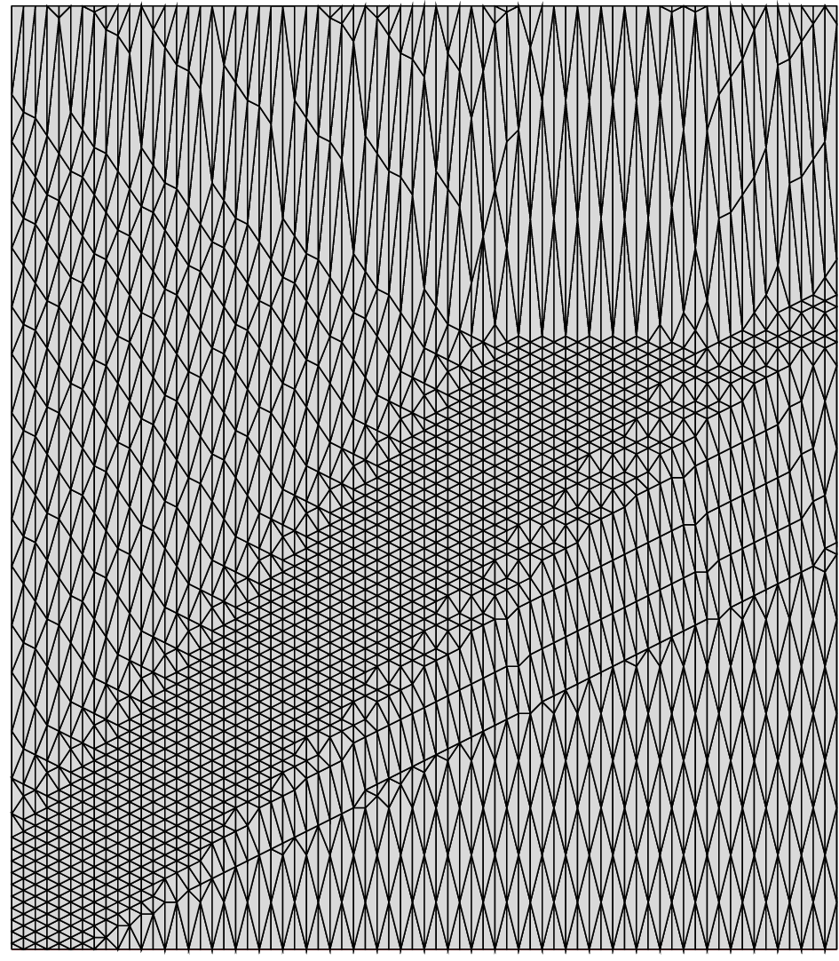
Figures 5 and 6 illustrate spacetime meshes constructed by our prototype implementation over 1D and 2D space meshes respectively. The 1DTime spacetime mesh was constructed by pitching an independent set of local minima in non-increasing order of wavespeed. In other words, the algorithm preferred to pitch local minima adjacent to points on the front where the wavespeed was maximum (slope was minimum). The 2DTime mesh was constructed by pitching a global minimum at every step. In either example, many more spacetime elements would be required to mesh the same volume if the height of every tentpole were constrained by the globally minimum slope.

In higher dimensions, we have a theorem identical to Theorem 7 when every dihedral angle of every simplex is non-obtuse. We anticipate soon an analogous theorem for arbitrary dimensional space domains in the presence of obtuse angles.
Our algorithm can be modified to handle asymmetric cones, such as due to wave propagation through anisotropic media. In the presence of anisotropy, the most limiting cone constraint can be nonlocal.
In a recent paper, Abedi et al. [1] extend TentPitcher to support another kind of adaptivity, where the size of the spacetime elements is adapted to a posteriori estimates of the numerical error. Abedi et al. apply hierarchical refinement and coarsening of the underlying one- or two-dimensional space mesh to adapt the spatial size of future spacetime elements. They extend the progress constraints of Erickson et al. to anticipate future refinement and coarsening both of which change the shape of the elements on the front. The outstanding problem that we plan to consider next is to combine adaptivity to changing wavespeeds with refinement and coarsening for the case of planar space domains. It is quite straightforward to combine the progress constraints in this paper with those of Abedi et al. to support refinement in the presence of changing wavespeeds. Coarsening can be done safely if each triangle after coarsening satisfies progress constraint []. When coarsening is possible only under such strict constraints, we need to carefully prioritize each coarsening step so that the front is only as refined as necessary and not much more.
Our research group is also implementing a parallel version of Tent Pitcher to run on multiple processors. The nonlocal nature of the constraints pose significant challenges in the parallel setting.
In many problems, the geometry of the space domain changes over time. There may also be internal boundaries between different parts of the domain, e.g., separating two distinct materials with different physical properties, and these internal boundaries may evolve over time. We would like to handle moving boundaries both internal and external.
Acknowledgments
The author would like to thank the other members of the CPSD spacetime meshing group, especially Jeff Erickson, Yong Fan, Robert Haber, Mark Hills, and Jayandran Palaniappan. Thanks also to the anonymous referee, whose comments were especially useful.
References
- [1] Abedi R., Chung S.H., Erickson J., Fan Y., Garland M., Guoy D., Haber R., Sullivan J.M., Thite S., Zhou Y. “Spacetime Meshing with Adaptive Refinement and Coarsening.” Proc. 20th Symp. Computational Geometry, pp. 300–309. June 2004
- [2] Barnes J.E., Hut P. “A Hierarchical Force Calculation Algorithm.” Nature, vol. 324, no. 4, 446–449, December 1986
- [3] Cockburn B., Karniadakis G., Shu C. Discontinuous Galerkin methods: theory, computation and applications, vol. 11 of Lecture Notes in Computational Science and Engineering. Springer, 2000
- [4] Erickson J., Guoy D., Sullivan J.M., Üngör A. “Building Space-Time Meshes over Arbitrary Spatial Domains.” Proc. 11th Int’l. Meshing Roundtable, pp. 391–402. 2002
- [5] Guttman A. “A Dynamic Index Structure for Spatial Searching.” Proc. ACM SIGMOD Conf. Principles Database Systems, pp. 47–57. 1984
- [6] Lin M., Manocha D., Cohen J., Gottschalk S. Algorithms for Robotics Motion and Manipulation, chap. Collision Detection: Algorithms and Applications, pp. 129–142. A.K. Peters, 1996
- [7] Lowrie R.B., Roe P.L., van Leer B. “Space-Time Methods for Hyperbolic Conservation Laws.” Barriers and Challenges in Computational Fluid Dynamics, vol. 6 of ICASE/LaRC Interdisciplinary Series in Science and Engineering, pp. 79–98. Kluwer, 1998
- [8] Richter G.R. “An explicit finite element method for the wave equation.” Applied Numerical Mathematics, vol. 16, 65–80, 1994
- [9] Üngör A. Parallel Delaunay Refinement and Space-Time Meshing. Ph.D. thesis, University of Illinois at Urbana-Champaign, October 2002
- [10] Üngör A., Sheffer A. “Tent-Pitcher: A Meshing Algorithm for Space-Time Discontinuous Galerkin Methods.” Proc. 9th Int’l. Meshing Roundtable, pp. 111–122. 2000
- [11] Yin L., Acharya A., Sobh N., Haber R., Tortorelli D.A. “A Space-time discontinuous Galerkin method for elastodynamic analysis.” B. Cockburn, G. Karniadakis, C. Shu, editors, Lecture Notes in Computational Science and Engineering, vol. 11, pp. 459–464. Springer, 2000