A novel canard-based mechanism for mixed-mode oscillations in a neuronal model
Abstract
We analyze a biophysical model of a neuron from the entorhinal cortex that includes persistent sodium and slow potassium as non-standard currents using reduction of dimension and dynamical systems techniques to determine the mechanisms for the generation of mixed-mode oscillations. We have found that the standard spiking currents (sodium and potassium) play a critical role in the analysis of the interspike interval. To study the mixed-mode oscillations, the six dimensional model has been reduced to a three dimensional model for the subthreshold regime. Additional transformations and a truncation have led to a simplified model system with three timescales that retains many properties of the original equations, and we employ this system to elucidate the underlying structure and explain a novel mechanism for the generation of mixed-mode oscillations based on the canard phenomenon. In particular, we prove the existence of a special solution, a singular primary canard, that serves as a transition between mixed-mode oscillations and spiking in the singular limit by employing appropriate rescalings, center manifold reductions, and energy arguments. Additionally, we conjecture that the singular canard solution is the limit of a family of canards and provide numerical evidence for the conjecture.
In this paper we investigate a specific biophysical model of a neuron, not previously analyzed, using techniques from dynamical systems theory. We discover the presence of mixed-mode oscillations (MMOs), alternating sequences of large amplitude (neuronal spikes) and small amplitude (subthreshold) oscillations, in the model. To explain the dynamical mechanisms responsible for the MMOs, we apply reduction of dimensions techniques to reduce the original model to a simplified model system with three timescales. Our analysis of this system leads to a novel mechanism for the generation of MMOs that is based on the presence of canard solutions that act as a transition between MMOs and spiking. The theory that we develop may be applied to systems from various contexts that exhibit mixed-mode oscillations and have the same underlying dynamical structure.
I Introduction
Mixed-mode oscillations (MMOs) refer to oscillatory behavior in which a number (L) of large amplitude oscillations is followed by a number (s) of small amplitude oscillations, differing in an order of magnitude, to form a complex pattern () of oscillations of varying amplitudes. MMOs were first noticed in the Belousov-Zhabotinsky reaction [1], and have been subsequently witnessed in experiments and models of numerous chemical [2, 3, 4, 5] and biological [6, 7, 8] systems. Recently there has been work on MMOs in models of neurons [9, 10, 11, 12, 13, 14]. In the context of neural dynamics, large oscillations correspond to firing of action potentials while small oscillations correspond to subthreshold oscillations (STO).
We have discovered MMOs in a biophysical model of a neuron in the entorhinal cortex (EC) introduced by Acker et al.[15]. The EC is thought to play a prominent role in memory formation through its reciprocal interactions with the hippocampus and participation in the generation of the theta rhythm (4-12 Hz) [16, 17, 18, 19]. Pyramidal neurons in layer V of the entorhinal cortex have been found to possess electrophysiological characteristics very similar to those seen in layer II stellate cells of the entorhinal cortex [20, 21], including their propensity to produce intrinsic subthreshold oscillations at theta frequencies. In layer V pyramidal cells these subthreshold oscillations are thought to arise from an interplay between a persistent sodium current and a slow potassium current [8, 7], while in layer II stellate cells, they are thought to arise from an interplay between a persistent sodium current and a hyperpolarization activated inward current () [22, 23, 12].
The model from Acker et al.[15] that we employ includes these currents and captures some dynamical aspects of the generation of STOs in layer V pyramidal cells. After a numerical investigation of the dynamics of the full model that displays the interaction of the persistent sodium and slow potassium currents to form STOs, we modify it by replacing the persistent sodium current by a tonic applied current. This can be interpreted as the modeling of an electrophysiological experiment designed to investigate the effects of blocking the persistent sodium current. The modified model displays MMOs, and the main focus of this work is to understand their nature. In order to simplify the analysis of the model, we perform a reduction of dimensions analysis [12, 24] to reduce the 6-d system into a 3-d system.
Among the proposed mechanisms for MMOs are break-up of an invariant torus [25], break up/loss of stability of a Shilnikov homoclinic orbit [26, 2] and subcritical Hopf bifurcation combined with a suitable return mechanism [27, 28]. Well known in the context systems with multiple time scales is the canard mechanism, introduced (to the best of our knowledge) by Milik and Szmolyan [3]. It is based on the presence of canards, which are defined as solutions that originate in a stable slow manifold and continue to an unstable slow manifold while passing through a thin region of non-hyperbolic behavior, which we refer to as the fold region. Primary canard solutions, that neither perform small amplitude oscillations nor spike, can act as dynamic boundaries between regions of small oscillations and spiking. Canard solutions have been analyzed in three dimensions using non-standard analysis by Benoit [29] and using techniques of geometric singular perturbation theory in combination with blow-up techniques by Szmolyan and Wechselberger [30, 31]. A general mechanism of MMOs based on the existence of canards has been postulated in [32]. There is a variety of different examples which, with some modifications, fit into the context of this general mechanism [31, 10, 3, 9, 11, 12, 13, 33, 14].
Our model fits into the context of a system with multiple timescales; we will show that the occurrence of MMOs in our model is related to the presence of canards. However, while in most of the other examples of canard mechanism small oscillations are due to rotations about a canard solution called the weak canard [32], in our case, during the stage of small oscillations, some of the trajectories follow closely the unstable manifold of an equilibrium of oscillatory type, very close to a Hopf bifurcation. In this aspect our system is similar to the systems studied in [2, 27, 28]. Consequently our model provides a novel mechanism for MMOs, one in which both canards and dynamics near a saddle-focus equilibrium play an important role.
We designed a three time scale model system that accurately reproduces most of the features of the neuronal model, and a significant part of this work is devoted to the analysis of the three time scale model equation. Most of the work, at least to some degree, relies on numerics. We show that canards can exist, but we conjecture they occur on parameter intervals of exponentially small width (, where is the ratio of the two slowest timescales). This is similar to the case of two dimensional canard explosion (known also as the canard phenomenon), where a small oscillation grows through a sequence of canard cycles to a relaxation oscillation as the control parameter moves through an interval of exponentially small width [34, 35, 36]. In contrast, in the two slow/one fast variable systems studied by Szmolyan, Wechselberger and others, canards occur in a robust manner, i.e., on open parameter intervals of size independent of the singular parameter. We also discover the role of canards in our system: we show (relying to some degree on numerics) that the transition from MMOs to pure spiking must correspond to a canard solution. We compute a canard numerically and compare the relevant parameter value to the parameter value of the transition from MMOs to spiking, finding that the two values are almost equal. We also calculate analytically the approximation of the numerically computed canard.
An outline of the paper is the following. In section II, we introduce the model and display the dynamical properties and bifurcation structure of the original Acker et al. model through simulations of the full system. We also perform a reduction of dimensions analysis to reduce the 6-d system to a 3-d system with three time scales in the subthreshold regime. In section III, we introduce the modification of replacing the persistent sodium current with a tonic applied current, and we analyze the mechanism for the MMOs observed in the modified model. We begin with a phase space description of the MMO activity through simulations. Next we propose a three time scale model problem, by adding an additional slower time scale to the model of Szmolyan and Wechselberger [30], and transform our system into this form. The three time scale model has a Hopf bifurcation and some of the dynamics in MMO sequences follows closely the unstable manifold of the unstable equilibrium, which reproduces well the behavior of the neuronal model. In our analysis of the MMOs in the three time scale model, a fundamental observation is that during the approach to the fold region the trajectories are attracted to a single trajectory, a 1-d (super) slow manifold contained in the attracting branch of a folded 2-d slow manifold. To investigate the flow near the fold curve, we perform an (singular perturbation parameter) dependent rescaling which blows up the flow near the fold curve. We define singular canards as solutions of this system satisfying certain asymptotic properties and find explicitly a singular canard that is a polynomial vector function of the independent variable. By employing appropriate rescalings, center manifold reductions, and energy arguments, we prove that a continuous family of canard solutions must converge, as , to a singular canard. Consequently, we prove that if a transition from MMO to spiking occurs along a continuous curve then must be a value for which a singular canard exists. We conjecture that the mentioned polynomial solution is the only existing singular canard and provide numerical evidence for this conjecture. We conclude with a discussion of related and future work in section IV.
II The model
II.1 Model equations
To investigate STOs and MMOs in EC layer V pyramidal cells, we consider a biophysical model introduced by Acker et al. [15] that includes two currents (persistent sodium () and slow, non-inactivating potassium () ) whose interaction is known to be responsible for the generation of STOs in these cells [8, 7]. In addition, the model contains the standard Hodgkin-Huxley currents [37]: transient sodium (), delayed rectifier potassium (), and leak (). The current balance equation for the model is given by
| (1) | |||||
where C is the membrane capacitance (), is the membrane potential (mV), is the applied bias current (), is conductance (), is the reversal potential (mV), and the time is in . Also, we define , , , , . The values of the parameters can be found in the Appendix. The dynamics of each of the gating variables and is described by a first order equation of the form
| (2) |
where represents the gating variable, represents the voltage-dependent time constant, and represents the voltage dependent steady state values of the gating variable. We will see that the and play an important role in the generation of subthreshold oscillations. The activation and inactivation curves for the gating variables are shown in Figure 1 while the voltage dependent timescales are shown in Figure 2.
II.2 Simulations of the full system
Simulations of the full system (1)-(2) show that the model fits into the category of class 2 neural excitability [38]. Using the applied current as a bifurcation parameter, the system undergoes a subcritical Hopf bifurcation as is increased as seen by Figure 3. Thus, as is increased, the cell switches between three different regimes . In the first regime (), there is a single stable rest state which is converged to through damped subthreshold oscillations. In the second regime (), there is bi-stability of the rest state and periodically spiking solutions, which are separated by unstable, small amplitude oscillations generated through a subcritical Hopf bifurcation (See Figure 4). The spiking solutions start with a minimal frequency of about 5Hz while the damped subthreshold oscillations have a frequency of about 10Hz. Also, the replacement of the slow potassium current with a tonic drive results in the absence of subthreshold oscillations (as in [8]) while the replacement of the persistent sodium current with a tonic drive will be discussed in section III. We note that the damped subthreshold oscillations involve the interplay of the slow potassium current and the persistent sodium current as seen in Figure 5. At the transition between the first and second regimes, we observe dynamics reminiscent of a 2-d canard phenomenon in which the trajectory shown follows a repelling unstable manifold. The third regime () consists of stable, periodic firing.
II.3 Reduction of Dimensions
We show that during the interspike interval, which corresponds to the subthreshold voltage regime, we can reduce the system to a 3-dimensional system (3). By analyzing the voltage dependent timescales seen in Figure 2, we see that . Thus, we seem to have three timescales with and evolving very quickly and evolving very slowly. Thus, letting and yields a reasonable approximation. By considering Figure 1 and 2, we see that when is hyperpolarized, evolves much faster to its steady state value (its time scale is 4 times smaller) than . Also, we note that . Thus, quickly approaches its steady state value , and then it can track it closely since changes very slowly during the interspike interval. Thus, we replace with and retain . Hence, we can reduce the system to one for which only and are dynamic variables.
To investigate the importance of the spiking currents (sodium and potassium), we also perform a bifurcation analysis. When is removed, the system exhibits a supercritical Hopf bifurcation in which sustained, stable subthreshold oscillations appear. (See Figure 6.) This change in the bifurcation criticality due to removal shows that the transient sodium current plays an important role in the interspike interval. With removed, the bifurcation structure is retained, but there is a significant shift in the Hopf bifurcation point (from to ). By retaining the equation, and replacing and with their steady state activation and inactivation functions and , respectively, we obtain the reduced 3d system
| (3) | |||||
where has been replaced by its constant value, . We note that the bifurcation diagram for this system (see Figure 7) is very similar to that of the full system.
Typically, the spiking currents are not included in the biophysical description of the subthreshold regime as in generalized integrate-and-fire models, which are constructed by biophysically describing the subthreshold regime using non-spiking currents and adding artificial spikes [39, 12]. This system provides an example where neglecting the spiking currents in the biophysical description of the subthreshold regime leads to a qualitative change in the cell’s dynamics, i.e. and must be included in this reduced system since our model is sensitive to small changes in the sodium and potassium currents during the latter part of the interspike interval before the spike. In some cases it has been shown that these currents play no critical role in the subthreshold regime [12].
III Analysis of mixed-mode oscillations
III.1 Simulations and outline of the results
We have discovered that in the full system (1-2) and in the reduced system (3) the replacement of the persistent sodium current with a tonic excitatory drive leads to mixed-mode oscillations in which a large amplitude spike is followed by a number of small amplitude subthreshold oscillations (see Figure 8). We note that this modified version of (3), with the persistent sodium current removed, exhibits a more complex bifurcation structure than (3) itself as seen in Figure 9. The system exhibits a single equilibrium which loses stability through a subcritical Hopf bifurcation at . For , the system exhibits continuous spiking. For between and , the system displays MMOs of type . For between and , the system displays MMOs with multiple STOs per spike, and the number of STOs per spike is a decreasing function of . Finally, for between and , the system exhibits sustained subthreshold oscillations.
Our goal is to analyze the mechanisms for this behavior in (3) with . We begin with a geometric interpretation of the MMOs using simulations of (3). We note that the v-nullsurface is a 2-d surface , and for fixed n, is a cubic shaped curve. Also, we note that (3) possesses a single fixed point, denoted by , which is near the fold curve of the v-nullsurface. The linearization about yields a large negative eigenvalue and a pair of complex eigenvalues with positive real part, and the ratio of the real eigenvalue to the real part of the complex eigenvalue is about -30. Thus, possesses a 1-d stable manifold and a 2-d unstable manifold. Numerical simulations show that a MMO trajectory travels down near the left sheet of the v-nullsurface (slow manifold) and subsequently passes near the fold, where it gets attracted to the 2-d unstable manifold of the fixed point . See Figure 10. The 1-d stable eigenspace of is plotted in red in the figures, and the plane displayed in the figures is the unstable eigenspace of . The trajectory approaches the unstable manifold of , which we denote by , along the stable manifold of . Then the trajectory spirals out from near along and continues to transversally pierce the v-nullsurface (the loss of alignment with the fast nullsurface during the passage through the fold region is typical for folded node or folded saddle node type dynamics), until it becomes tangent to the v-nullsurface. At this point, the trajectory leaves and gets attracted to the right sheet of the v-nullsurface since it enters a region in which is strongly repelling from the left sheet. Then, there is a return mechanism (spiking regime) that brings the trajectories back to the left sheet of the v-nullsurface. We note that the feature of a passage near the unstable manifold of a saddle focus equilibrium followed by a reinjection mechanism is reminiscent of Shilnikov’s example [40] as well as of the examples where MMOs occur through a subcritical Hopf bifurcation [27, 28] (see section IV for a detailed discussion).
In the remaining part of this work much of the focus will be on the following model system
| (4) | ||||
where is small and is a control parameter. System (4) shares many of the features of (3) but is a lot simpler. The initial part of our analysis is to establish two basic geometric features of the flow:
- 1.
There exists an equilibrium of oscillatory type, which loses stability through a Hopf bifurcation for close to .
- 2.
The critical manifold is a surface with two fold lines. There exists a 2D attracting slow manifold close to one of the sheets of this surface, and within this slow manifold there is a 1D super-slow manifold, approximating the curve , .
We will show that all the MMO trajectories must pass very close to the super-slow manifold. Consequently, the distance between the continuation of the super-slow manifold to the fold region and the stable manifold of the equilibrium is of great importance for the nature of the MMOs. If this distance is small, then the trajectory must follow for a long time the flow along the 2D unstable manifold of the equilibrium, making many rotations about the equilibrium. As this distance increases, the role of the unstable manifold of the equilibrium diminishes.
In this work we have focused on the transition from MMOs to spiking. This occurs in the parameter regime where the continuation of the super-slow manifold, and thus the MMO trajectories, are relatively far from the equilibrium. We have been able to show, with the help of some numerics, that the transition from MMOs to spiking occurs through a canard, and that families of canard solutions converge to singular canards, which are special solutions of a suitable limiting system. We have also found a parameter value for which a special solution exists. We conjecture, based on numerical evidence, that this parameter value is unique.
III.2 Derivation of the model system
In order to investigate MMOs in system (3), we transform it to a three timescale toy model of the form
| (5) | |||||
with and . To this end, we begin by first treating (3) as a slow-fast system with two timescales in order to obtain a folded singularity, which we will use as the origin for our model system in order to study small amplitude oscillations near the fold curve of the 2-d folded v-nullsurface of (3). For an exposition on folded singularities, see [30, 31].
Two timescales are uncovered by dividing the equation of (3) by the maximum conductance and setting we obtain
| (6) | |||||
where for , and and . We note that the conductances in the equation are bounded by 1 and the magnitudes of the and equations are bounded by 1 since and . Thus, evolves on a faster time scale then or . Momentarily, we neglect the fact that and vary on different timescales.
By setting , we obtain the reduced system which is a 2-d dynamical system on the critical manifold . Based on the work of [30, 31], we wish to show that is a non-degenerate folded surface in the neighborhood of a folded equilibrium point with . In order to compute , we begin by solving for and obtain . Next, we solve for as a function of and find that is a constant, which we denote by , along the fold curve (since and are linear in and ). Also, we denote by . Thus, the fold curve is parametrized by , . Also, we differentiate with respect to to obtain . Thus, the reduced 2-d system on the critical manifold can be denoted by
| (7) | |||||
where is replaced by . Through a solution dependent time rescaling we obtain the desingularized reduced system
| (8) | |||||
We numerically solve for with and to obtain . Finally, . We note that is a fixed point of (7) and (8). We linearize (8) about this fixed point and find that in our parameter regime both eigenvalues are negative, resulting in a folded node equilibrium. We note that the quotient of these eigenvalues predicts the maximum number of subthreshold oscillations per spike [30, 31] for sufficiently small. However, this prediction is incorrect (underestimate) for this system since there are three timescales, resulting in a that is not sufficiently small in the two timescale formulation.
We now shift the folded node point to the origin in (6) with the transformation , , and to obtain
| (9) | |||||
Next, we rectify the fold curve to the axis. We note that the fold curve is parametrized by . where . Thus, we make the substitution , , and to obtain
| (10) | |||||
We note that .
Then we let , , and where and to obtain
.
| (11) | |||||
To simplify the equation we let , , and to obtain
| (12) | |||||
Next, we rescale time with , let and , and truncate higher order terms to obtain
| (13) | |||||
Finally, if we let , then we obtain
| (14) | |||||
where , , and . This system is equivalent to (5). For example, if in (3), the parameters are approximated by: , and . Also, we consider , which provides an appropriate return mechanism. A more general assumption that we make to guarantee the desired functioning of the toy model is
| (15) |
III.3 Slow manifolds of the model system
Equation (5) has a two dimensional critical manifold defined as the set of equilibria of (5) with set to . We denote this manifold by and note that it is defined by the equation . Let denote the unique value of for which the function has a maximum. Let
where and denote attracting and repelling, respectively. By Fenichel theory [41], away from the fold lines and , , system (5) with has locally invariant manifolds and that are close to and . While the existence of and is standard and not surprising, we also argue that there exists a one-dimensional super-slow manifold (it can be chosen to be contained in ), denoted by , that attracts all the dynamics on . (See Figure 11.) For this reason it is convenient to rescale (5) to the slow time scale, which gives (4). Setting , we obtain two constraints:
This gives a one dimensional curve defined by:
| (16) | ||||
which we denote by . Note that assumption (15) guarantees that the flow on is towards the fold.
Linearizing (4) about we obtain the matrix
Ignoring the terms in we obtain
It is easy to verify that this matrix, apart from an eigenvalue , has eigenvalues and , which are both negative for . It follows that the dominant eigenvalues of are
There is also a third eigenvalue, which is , but we are interested only in the two leading ones. By a slight modification of Fenichel theory we can prove that (5) has a one dimensional attracting locally invariant manifold, which we denote by . All the trajectories which make a relaxation loop (spike) must become exponentially close to it before they enter the fold region. Thus, there is a single trajectory that needs to be tracked through the fold region to determine the existence of MMOs/small amplitude dynamics and this trajectory can be arbitrarily chosen as long as its initial condition is not too close to the fold. We illustrate this scenario in Figure 12 in which we display along with a spiking solution for that tracks quite closely as well as a MMO solution for the larger value of .
III.4 The microscope: a rescaling of the model system
In order to understand the flow of (5) in the fold region, we introduce a rescaling which blows up a rectangle of size to the size of in each of the directions. This trick has been widely used in the study of canard problems and was given the name ’microscope’ by Benoit, Diener and others who investigated canard explosion and related problems by means of non-standard analysis [42, 29, 43]. In the case of (5), the ’microscope’ rescaling is as follows:
Remark 1
In Proposition 1 we will prove that MMOs cannot exist if is too large. This implies that MMOs exist for only.
After rescaling the variables we obtain the following system:
| (17) | ||||
By setting we obtain:
| (18) | ||||
Remark 2
A similar normal form arises in the study of folded node [29], [30]. The difference is in the equation, where the terms and do not appear. However these two terms alter the dynamics dramatically, so that the results on the folded node normal form cannot be easily applied in the context of (18). We have some partial results in the direction of reducing the study of the dynamics of (18) to facts about the dynamics of the normal form of folded node, but the arguments are very technical and it does not seem worthwhile to present these results in this paper.
The system (18) has a unique equilibrium given by
The linearization at the equilibrium is given as follows:
with . We assume that , which implies that the determinant is always negative. Clearly the only way for the matrix to be non-hyperbolic is if there is a pure imaginary eigenvalue. Let denote the characteristic polynomial of and note that can be written in the form . The condition for to have a purely imaginary eigenvalue is . We evaluate the coefficients and get
We define the function by the formula
Clearly the roots of give purely imaginary eigenvalues. Evaluating we get
Now has two roots, given by
For example, if and (corresponding to ), the two roots are and . The first corresponds to the Hopf bifurcation point while the second is an extraneous solution.
III.5 Special solution
System (18) has special solutions that are algebraic as , i.e. solutions that tend to no faster than a polynomial function of . In this section we will prove that for each value of there exists exactly one such solution (up to time rescaling). The importance of special solutions will become clear in Section III.6 where we will show that the continuation of the manifold to the region of validity of the ’microscope coordinates’ is close to the special solution of (18) corresponding to the same value of .
In order to understand the flow of (18) near infinity, including special solutions, we make the following transformation:
| (19) |
The transformation yields the following system:
| (20) | ||||
Through an appropriate (solution dependent) time rescaling we can eliminate a factor of in (20):
| (21) | ||||
Solutions of (21), suitably reparametrized, become solutions of (20), except of course for the solutions for which . Equation (21) has two lines of equilibria, given by
| (22) |
These lines of equilibria were artificially introduced by the time rescaling which led from (20) to (21). The reason for making the transformation was to remove the singularity created by the term . The resulting system (21) can be analyzed using dynamical systems theory. Namely, we can understand the flow near the line of equilibria, thus obtaining insight into the structure of solutions of (20). We focus on the line of equilibria with since it corresponds to the attracting direction. Observe that there exists a center manifold containing the line of equilibria. We denote this center manifold by . Note also that points on satisfy the constraint by center manifold theory [44]. Substituting into (21), we obtain
| (23) | ||||
Now we can introduce the ”inverse” of the time rescaling which lead from (20) to (21), by reducing a factor of . Thus we are back to the original time coordinate. The resulting system is
| (24) | ||||
System (24) has an equilibrium at , which has one stable direction and one center direction. The branch of the center manifold existing for , which we denote by , is unique. Equation (24) restricted to has the form
| (25) |
and gives a solution of (20) and thus of (18) which is algebraic in backwards in time. All other solutions of (20) grow at least exponentially as . We will denote the special solution in the coordinates by .
We now look for a special solution of (18) which is a polynomial vector function in . Suppose that is a polynomial solution and note that it can only exist if and are linear in and is quadratic in . We can write
Using the first equation in (18), we obtain
Substitution into the second equation in (18) results in
Finally, the third equation in (18) gives
from which we get the conditions
Solving we get
It follows that a polynomial solution exists for with
Note that transformation (19) takes solutions with algebraic behavior as to solutions with algebraic behavior as . Consequently, by uniqueness of , . We denote the value of corresponding to by .
Remark 3
We could repeat the construction of the beginning of this section to obtain special solutions which are algebraic as . For each there exists exactly one such solution. Typically the special solutions for do not match with the special solutions for . The number is an exceptional value of for which the two kinds of special solutions are equal; the corresponding solution is . In Section III.10 we will present numerical evidence that is the limit of a family of canard solutions.
III.6 Continuation of into the fold region
In Section III.3 we proved that all trajectories on are attracted to a one dimensional manifold . Naturally and its flow continuation play a crucial role in the organization of the dynamics of (5). In this section, we show that any solution with initial condition on , when it passes through the region of validity of the coordinates, must be close to the special solution .
As in Section III.5, we use the coordinate transformation (19), but we apply it to equation (17) here. This yields
| (26) | ||||
Subsequently, we apply the time rescaling resulting in the removal of the factor :
| (27) | ||||
Notice that setting in (26) (resp. (27)) gives (20) (resp. (21)).
We now note that
where are the coordinates introduced in (19). Consider a point close to the fold region and let be the corresponding point in the coordinates. By (16), is close to the curve . We fix small, which corresponds to the assumption that is close to the fold region. Observe that is close to . We investigate the solution of (27) with initial condition .
Consider the following system of equations:
| (28) | ||||
Note that (28) has a constant of motion , and that (27) is a reduction of (28) to the invariant hypersurface .
We now argue in a similar way as in section III.5:
- •
there exists a center manifold satisfying the constraint . We denote this manifold by because, even though it is three dimensional in the context of (28), it is two dimensional in the variables , i.e. once the reduction has been implemented. The manifold can be viewed as a center manifold of the 2D surface of equilibria defined by and .
- •
restricted to we can rescale the time and find a 2D center manifold, denoted by , which is a natural generalization of to the case. That is, center manifold theory guarantees the existence of functions such that is defined by the equations
(29) and is defined by the equations
(30) (Recall that corresponds to the special solution.) The flow on is given by
(31) and the level curves of the function are invariant. (This system is the analogue of (25) in the case.)
We define two sections of the flow of (28):
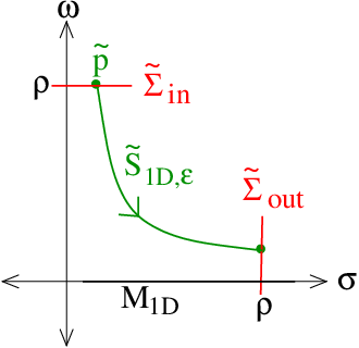
where is the constant used in the definition of the point . (See Figure 13.) We are interested in describing the transition by the flow of (28) from to . We state a few important properties of (28):
- 1.
The manifold is strongly attracting. To see this, recall that is an attracting center manifold of the line of equilibria defined by , .
- 2.
The manifold is also attracting, since it is an attracting center manifold in the context of the system obtained by restricting (28) to and cancelling a factor of (similar construction as leading from (23) to (24)). The attraction rate is weaker, but since the solutions on move fairly slowly, solutions with initial conditions off in are very close to in .
- 3.
Consider a trajectory of (28) starting in . Since is contained in the invariant hypersurface , it follows that it must approach the intersection of with the attracting manifold . Since this is a one dimensional curve containing no singularities, it must be a trajectory. Hence it follows that approaches a specific trajectory on .
- 4.
By the definition of and due to the constraint we have , which, together with (30) implies that the distance between and is . Let be defined by the requirement . It follows that converges to as .
It follows from points 1. and 2. that the transition map from to , defined by the flow of (27), mapping a neighborhood of to a neighborhood of , is a strong contraction. We can conclude this because the restriction of the flow of (28) using the constraint to the flow of (27) amounts to factoring out the neutral direction.
Remark 4
The manifold as we defined it (center manifold of the surface of equilibria given by and for (28)) is not unique. We add a requirement that equals in the section . This way is the continuation of in the coordinates. Recall that is strongly attracting, which means that it inherits the stability property of . The procedure of extending slow manifolds into the flow region is described in detail in [34].
III.7 The manifolds and
In the preceding section we constructed and analyzed the manifold as the continuation of in the coordinates. In this section we carry out an analogous procedure, namely we find a manifold that extends the unstable slow manifold backward in time. Note that (28) has a equilibria given by the conditions and . Let be a center manifold of this surface of equilibria. This manifold satisfies the condition
| (32) |
The manifold is foliated by two dimensional surfaces , defining invariant submanifolds of (27).
We now substitute the constraint (32) into the subsystem of (28) and cancel a factor of , analogously to the derivation of (23) from (21). We obtain:
| (33) | ||||
The system (33) has an attracting two dimensional invariant manifold given by condition (32) and
The manifold defines one dimensional submanifolds of (28) via the constraint . The manifold , as defined, is not unique. We add the requirement that is equal to in the section (see Remark 4). A very important feature of is that is contracting forwards in time, which means that if the manifold is continued backwards in time, the direction is rapidly expanding. In the limit there exist manifolds and of (21) that are analogous to and .
III.8 A bound for the MMO behavior
As mentioned in Section III.4, MMOs cannot exist if is too large. In other words, the region of the the existence of MMOs in the parameter must be in size. Here we state and prove the relevant result.
Proposition 1
There exists and such that for and no MMOs can exist.
Proof By the analysis of Section III.6, we know that solutions originating in , transformed to the variables , satisfy and . By assumption (15), we have for sufficiently small and . By possibly decreasing the bound on , we can make sure that is satisfied even when we increase (see (28)). We transform to the variables at , where is very small and possibly depends on . The corresponding value of is . We carry out the remainder of the argument for system (18), leaving the generalization to (17) to the reader.
We choose a constant satisfying so that we can make a “tube” around the parabolic cylinder , with the top and the bottom given by and so that the solutions can exit the tube only through the bottom. We define as sides of the tube the parabolic cylinders , where is a small constant, and leave the tube unbounded in the direction. For the moment we restrict attention to the part of the trajectory for which (and ). We now prove that if and are sufficiently large, the trajectories cannot exit the tube through the sides. Note that due to in (18), we obtain on with in both cases. If is sufficiently large, the sides of the tube are almost vertical, and the component of the vector field restricted to the sides of the tube is almost horizontal and must be pointing towards the interior of the tube. It follows that trajectories can only exit through the bottom, as claimed. By increasing we can guarantee that when the trajectory reaches the bottom of the tube.
Now note that will remain non-negative. Also, as long as remains non-positive, must decrease and (since ). However, cannot reach as long as is positive. Also, since we must have . Hence, . It is now easy to estimate that the time T need for to reach satisfies
By taking sufficiently large we can guarantee that by the time reaches , must become at least . By increasing we can also make arbitrarily large. Since will not decrease, it follows that must become at least equal to before starts increasing. It is well known that for any initial condition with , , and sufficiently large the solution must enter a relaxation loop [34]. Hence, no STO (which requires to increase and to decrease) can exist.
III.9 Canard solutions and the boundaries of MMO behavior
In this section we discuss the role of canards in transitions between different MMO regimes. We explain in more detail what we mean by MMOs and canards and discuss how transitions between different MMO regimes can occur. We identify one type of the possible transitions as occurring through a canard and present numerical evidence showing that the final transition to spiking must be of this type. Finally we discuss the limit of canards in the variables and show that they correspond to singular canards that are special solutions of (18). An explicit example of such a special solution is the algebraic solution found is Section III.5. We conjecture that the value corresponding to is the limit of the values where the transition between MMOs and spiking occurs.
We begin by giving a more precise meaning to MMOs and canards. Let be the interior of the cube , where is some fixed small number. Consider a trajectory originating near outside of V (with the initial value of ). We say that has rotation type if has non-degenerate maxima and minima during the passage of the trajectory through . A trajectory originating in is a th secondary canard if has non-degenerate maxima and minima during the passage through and subsequently continues into . A primary canard is a trajectory that passes through with monotonically increasing () and subsequently continues into .
Before we discuss MMOs and their transitions, we point out a difference between (14) and the folded node problem [29, 30, 31]. Recall the one dimensional invariant manifold contained in . It was shown in Section III.3 that all trajectories on are attracted to . We define an canard as a trajectory originating in and continuing to . Note that an canard corresponds to an intersection of a 1D invariant manifold and 2D invariant manifold . If such an intersection is transverse with respect to the variation of (i.e. in the 4D extended phase space including ), then crosses from one to the other side of . If we knew that all the intersections were transverse, we could conclude that canards exist only for isolated values of . Suppose that is a canard solution that is not an canard (the initial condition is not contained in ). Since , during its passage along , becomes exponentially close to , it follows that the (minimal) separation between and must be exponentially small. Consequently, if we knew that the distance between and as a function of were not identically equal to 0 and varied at least algebraically in , we could conclude that canard trajectories can only exist on exponentially small (), ) intervals of the parameter . By contrast, in the folded node problem, canards exist robustly (for all the values of the control parameter) [29, 30, 31].
We now consider transitions between different types of MMOs. We will restrict attention to MMO periodic orbits of type , i.e. small loops followed by a spike. More precisely, we consider MMO periodic orbits with rotation type (see the definition above). If we change then the rotation type can change in two ways:
- (a)
-
Either a large loop can decrease in size and become fully contained in , or a loop contained in can grow and be no longer contained in .
- (b)
-
For some intermediate value of , has a degenerate critical point corresponding to the collapse of a small loop.
The following result shows that if a certain non-degeneracy condition holds, then all the transitions are of type (a). Moreover, they correspond to transitions through a canard.
Proposition 2
Suppose there exist two MMO periodic orbits with rotation type and , respectively, for two different values of , denoted by and , respectively. Recall the special solution and assume that for any has only non-degenerate critical points. Then, provided that is sufficiently small, the transition between the two MMOs is through a canard.
Proof Let and denote the MMO with rotation type and , respectively. Suppose we vary from to . Given a trajectory of (5), note that a critical point of corresponds to a crossing with the nullsurface . At such a critical point we have , so that a degenerate critical point can only occur if . If the solution crosses the nullsurface outside of and close to , then the solution must have followed for a significant amount of time so that . Thus , by Proposition 1. Hence, for sufficiently small, the critical point must be non-degenerate. Now we consider a crossing of the x-nullsurface inside of V. Any such crossing point must also be non-degenerate, due to the assumption on (by compactness and smooth dependence on initial conditions, the intersections of with must also be non-degenerate). For outside of a bounded region we switch to the coordinates and observe that, in order to reach the nullsurface, the trajectory would have to follow , and therefore be attracted to , so that would have to hold (see Section III.7), making impossible since . We have proved that all the crossing points with the nullsurface must be non-degenerate. It follows that the only way a transition from to can occur is if a point of intersection of the trajectory with the nullsurface traces the entire nullsurface until one of the small loops develops to a spike.
Although we believe that all the intersections of with the nullcline (for system (18) are transverse, we have only partial results in this direction, and we feel that they are not suitable for this article and will be presented in future work. Here we state the following conjecture.
Conjecture 1
The least for which (for system (18)) corresponds to a transverse intersection.
As support for this conjecture we have plotted the value of at the first intersection point of with the surface in Figure 14.
Remark 5
The following result concerns the limit of canards in the context of (17). We say that the special solution (18) is a singular canard if it continues to .
Theorem 1
Proof Recall that in Section III.6 we showed that the continuation of to the fold region must be close to the special solution . As shown in Section III.7, equation (26) has a 2-d repelling invariant manifold , which is a continuation of to the fold region (backward in time). In the limit we obtain a two dimensional invariant manifold of (20), which we denote by . A canard solution, as it passes through the fold region, must become exponentially close to , and then connect to , before going on to . In the limit we get a connection from to . The value corresponding to an limit of a transition from MMOs to spiking has to be one for which such a connection exists. Note that the validity of this argument relies on the convergence of the continuation of to the special solution in the variables . The relevant convergence result was established in Section III.6.
Remark 6
The defining property of a singular canard, namely continuing to , is non-generic and is likely to occur for isolated values of (provided that a suitable transversality condition holds). We know one example, with , corresponding to the polynomial vector solution . We conjecture that is the limit of the locus of the transition from MMO to spiking. This conjecture will be presented in more detail at the beginning of the next section.
III.10 Transition from MMO to spiking – numerical results
We propose that is the unique singular canard and that it persists as a regular canard, that is a connection between and . Consequently, we conjecture the following:
Conjecture 2
There exists a function such that for system (5) has a primary canard. The transition from MMOs to spiking occurs within an exponentially small (, ) interval of about . Moreover,
We investigate this conjecture numerically by first considering the transition threshold between MMOs and pure spiking in system (17) by computing solution trajectories for decreasing values of and near The simulations show that for decreasing values of , the transition between MMOs and pure spiking occurs for decreasing values of and suggest that as as seen in Figure 15.
In addition, we have found an approximate primary canard numerically. As noted above, such a solution must become exponentially close to the attracting manifold as it passes through the fold region and then connect to the repelling manifold before going on to . We exhibit this numerically using the Poincare section option of XPPAUT (Ermentrout02) for . That is, we choose an initial condition with on the singular primary canard and integrate until reaching the Poincare section . See Figure 16. This solution is expected to become exponentially close to . Next, we approximate by choosing a range of initial conditions varying in with , , and near and integrating backwards in time up to the Poincare section at to form a family of curves which form an approximation of . As shown in Figure 16, an approximate connection between these manifolds is obtained for . The approximate primary canard solution that corresponds to the intersection of these two manifolds and shows the characteristic long term (O(1)) following of a repelling manifold is also displayed in Figure 17.
Additionally, numerical simulations with varying levels of show a transition between MMOs and spiking near the value of for the approximate primary canard as seen by the MMO solution trajectory for and the spiking solution for in Figure 17. Thus, our numerical simulations support the validity of the persistence of the primary canard as stated in Conjecture 2.
There are many other interesting issues to analyze in this model including the transition from small amplitude dynamics to MMOs and the rotation properties of MMOs. For example, one could try to obtain an approximation for the number of subthreshold oscillations per spike for a given value of . We discuss such issues in the Discussion, but a detailed analysis of these issues is beyond the scope of this paper.
IV Discussion
In this work, we have analyzed a model introduced by Acker et al.[15] to study synchronization properties of stellate cells in layer II of the entorhinal cortex (EC). We were interested in studying subthreshold oscillations in pyramidal cells of layer V of the EC. Since there was no available model of EC layer V pyramidal cells at the time, and since the two cell types exhibited very similar electrophysiological characteristics, including the presence of persistent sodium and slow potassium currents that are thought to underlie the dynamics of STOs, we chose to employ the Acker model to model STOs in layer V pyramids. We note that layer V pyramidal cells exhibit many other interesting dynamical properties. They participate in high frequency ( Hz) ”ripple” activity associated with hippocampal sharp waves [45] and are a site of initiation and propagation of epileptiform activity[46]. Also, they exhibit graded persistent activity, which is associated with memory processes, in which neurons respond to consecutive stimuli with graded changes in firing frequency that remain stable after each stimulus [47]. In 2006, Fransen et al. introduced a quite detailed multi-compartmental model of layer V pyramidal cells that exhibit the graded persistent activity. In future work, we plan to adapt our analysis of the simpler model considered here to this more realistic model, and analyze the dynamics of the graded persistent activity.
We began our work with a numerical investigation of the dynamical properties and bifurcation structure of the full model and displayed the role of the persistent sodium and slow potassium currents in the generation of subthreshold oscillations. In order to analyze the 6-d system, we performed a reduction of dimension analysis to reduce the system to a 3-d system. We note that a more thorough reduction of dimensions analysis of a similar model of a layer II stellate cells with an h-current and persistent sodium current was performed by Rotstein et al. [12], and a computational tool for reducing systems possessing multiple scales has also been developed [24]. Rotstein et al. have also analyzed MMOs present in that model [13].
Just as experimental neuroscientists often modulate or block various currents in order to learn about their role by observing the effects of their absence, we investigated the effect of modulating various currents in our model. Upon removing or reducing to a very low level the persistent sodium current and replacing it with a tonic excitatory input, we witnessed very interesting dynamical phenomena including MMOs and seemingly chaotic firing patterns. (Future work includes the investigation of whether our analysis and the dynamical mechanism involved carry over to the case where a small persistent sodium current is retained.) This experiment is unable to be performed presently in the lab since there are no known drugs which are able to selectively block persistent sodium current without blocking the standard sodium current, and we felt it would be interesting to investigate this regime, especially due to the rich dynamical behavior present. The main focus of this work is to explain the dynamical mechanisms responsible for the mixed-mode oscillations.
We have discovered and analyzed a novel dynamical mechanism for the generation of MMOs, involving the canard phenomenon as well as the dynamics near a saddle focus equilibrium, as in the Shilnikov scenario [48] or the subcritical Hopf scenario [27, 28]. The techniques we employed to analyze the MMOs involve standard techniques from dynamical systems theory such as geometric singular perturbation theory [49, 50, 34] and center manifold theory [44]. For a summary of the analysis, see the last paragraph of section I.
A main accomplishment of this work is an analytical expression for the parameter at which the transition between MMOs and spiking occurs in the singular limit and a characterization of the corresponding singular primary canard solution responsible for the transition. Moreover, we construct a well developed geometric picture of the dynamics for this new canard-based MMO mechanism since we utilize a great deal of the underlying geometric structure available including slow manifolds, canards, and the saddle-focus equilibrium with its weak unstable manifold. In addition, the use of the folded-node point from the two time scale model to derive our novel three time scale model is new. Also, our analysis, which resulted from the investigation of a neuronal model, is applicable to studying MMOs in other systems from various contexts that have the same underlying dynamical structure, i.e. systems that can be transformed into the form of (5).
Prominent among scenarios for MMOs not involving canards are the Shilnikov scenario [40, 2, 51] and the subcritical Hopf scenario [27, 28]. Both involve a saddle focus equilibrium with a two dimensional unstable manifold and a return mechanism of ’soft reinjection’, which basically means that the return mechanism is given by a typical orientation preserving diffeomorphism. Our model system (5) has a saddle focus equilibrium with a weak unstable manifold, but in addition it has a multiple time scale structure, folded critical manifolds, and a singularity similar to a folded node. One of the consequences is that the return mechanism is not soft, but has a definite structure determined by the slow manifolds. Moreover, as we have demonstrated in the paper, the multiple time scale structure influences subthreshold oscillations by means of canard solutions.
It follows from our analysis that all the orbits leaving the vicinity of the saddle focus equilibrium will be attracted to the super-stable slow manifold, which returns to the vicinity of the equilibrium. Thus the system can be viewed as close to a homoclinic bifurcation. In this paper we have concentrated on the aspects of the problem related to the canard mechanism, but we feel that the methods employed to study homoclinic bifurcations, and especially the passage near a saddle point, may be applicable and useful for a more detailed investigation of our problem. We intend to explore the homoclinic-like features of the problem in future work.
In future work, we also intend to analyze the rotational properties of the solutions of (5). For a solution originating in or nearby, we define its rotation number to be the number of small loops it makes while passing through the fold region, which we define as a sufficiently large ball centered at the origin in the coordinates . Note that due to the strong attraction of , all the solutions entering the fold region will have the same rotation number, unless the system is very close to a canard. Here we mean a primary canard or a secondary canard, as secondary canards correspond to boundary curves, in the parameter space, between parameter regions for which solutions have different rotation numbers. We conjecture that for a fixed , there is a sequence of values, corresponding to secondary canards with increasing and to transitions corresponding to an increment by in the rotational number, ending with a region corresponding to the maximal number of rotations beyond which only small amplitude dynamics exists. Also, we have not analyzed the transition from small amplitude dynamics to MMOs. We know from simulations that small amplitude chaos is present, and we conjecture that it is related to the loss of normal hyperbolicity of the unstable manifold of the saddle-focus equilibrium, which must occur sufficiently far away from the equilibrium. Also, we believe that it is related to the Shilnikov scenario involving incomplete homoclinicity.
Another interesting question is how to estimate the rotation number for given values of and . Unfortunately, we do not foresee that an analytic formula can be obtained, in contrast to related cases in which there are two timescales [30]. A conjecture very strongly supported by the numerics is that the rotations happen almost exclusively during the slow drift of the solutions along the unstable manifold of of the saddle focus equilibrium. We also believe that the flow along this unstable manifold is close to its linear approximation. Once the solutions come to a region where and/or are sufficiently large, the unstable manifold loses normal hyperbolicity and the multiple time scale nature of the system takes over, thus ending the rotational phase of the solution. However, in order to produce an approximate formula for the number of rotations, one would need to know the distance from the continuation of to the stable manifold of the saddle focus equilibrium, measured in a specified section such as the hyperplane , as well as the distance between the equilibrium and the region where normal hyperbolicity is lost. One would also need the information on the eigenvalues and the eigenvectors of the saddle focus equilibrium. No analytic version of the formula can be expected since it seems quite unlikely to obtain an analytic formula for either the continuation of all the way to the section or the stable manifold of the saddle focus equilibrium, but a numerical formula seems achievable.
Note that even in the case of [30], only a formula asymptotic in is available, and in fact the formula of Szmolyan and Wechselberger is the approximation. In our case, we can consider an asymptotic formula based on the linear approximation of the flow along the unstable manifold, and in the approximation this would mean that would be used instead of the continuation of . However, again no analytic formula can be expected as no analytic expression for is available, except for the special case where . A possibility would be to obtain an asymptotic expression using center manifold theory, along the ideas of Section III.5, and we plan to pursue this idea in future work.
V Appendix
V.1 Model equations
The full model for the layer V pyramidal cell is given by
| (34) | |||||
The default parameters for the system are: , , , ,
, , , , and .
The graphs of the voltage dependent activation and inactivation functions as well as the voltage dependent time constants are given in Figures 1 and 2, and
their equations are the following:
where
and
.
where
and
.
where
and
.
.
.
The equations for the voltage dependent time constant for is:
.
VI Figures




Acknowledgements.
The authors are deeply indebted to Nancy Kopell for her numerous contributions to the paper. The authors would also like to thank Nicola Popović, Martin Wechselberger, and the reviewers for fruitful discussions. The research of MK was supported in part by NSF grant DMS-0406608. The research of JJ was supported in part by a YSU Research Professorship.References
- [1] A.M Zhabotinsky. Periodic kinetics of oxidation of malonic acid in solution. Biofizika, 9:306–311, 1964.
- [2] M.T.M. Koper. Bifurcations of mixed-mode oscillations in a three-variable autonomous van der pol-duffing model with a cross-shaped phase diagram. Physica D, 80:72–94, 1995.
- [3] A. Milik, P. Szmolyan, H. Loffelmann, and E. Groller. Geometry of mixed-mode oscillations in the 3d-autocatalator. Int. J. Bif. Chaos, 8:505–519, 1998.
- [4] I. R. Epstein and K. Showalter. Nonlinear chemical dynamics: oscillations, patterns and chaos. J. Phys. Chem., 100:13132–13147, 1996.
- [5] H. G. Rotstein and R. Kuske. Localized and asynchronous patterns via canards in coupled calcium oscillators. Physica D, 215:46–61, 2006.
- [6] T.R. Chay, Y.S. Fan, and Y.S. Lee. Bursting, spiking, chaos, fractals, and universality in biological rhythms. Int. J. Bifurc. Chaos, 5:595, 1995.
- [7] C.T. Dickson, Magistretti J., Shalinsky M., Hamam M., and Alonso A. Oscillatory activity in entorhinal neurons and circuits. Annals New York Academy of Sciences, 911:127 – 150, 2000.
- [8] M. Yoshida and Alonso A. Cell-type specific modulation of intrinsic firing properties and subthreshold membrane oscillations by the m(kv7)-current in neurons of the entorhinal cortex. J. Neurophysiol., accepted.
- [9] G. Medvedev and J. Cisternas. Multimodal regimes in a compartmental model of the dopamine neuron. Physica D, 194:333–356, 2004.
- [10] J. Drover, J. Rubin, J . Su, and B. Ermentrout. Analysis of a canard mechanism by with excitatory synaptic coupling can synchronize neurons at low firing frequencies. SIAM J. Appl. Math, 65:69 – 92, 2004.
- [11] J. Rubin and M. Wechselberger. The selection of mixed-mode oscillations in a Hodgkin-Huxley model with multiple timescales. Chaos, 2007.
- [12] H. G. Rotstein, J.A. Oppermann, T.and White, and N. Kopell. The dynamic structure underlying subthreshold activity and the onset of spikes in a model of medial entorhinal cortex stellate cells. J. Comput Neurosci., 21(3):271–92, 2006.
- [13] H.G. Rotstein, M. Wechselberger, and N. Kopell. Canard induced mixed-mode oscillations in a medial entorhinal cortex layer ii stellate cell model. submitted.
- [14] M. Krupa, N. Popović, H.G. Rotstein, and N. Kopell. Mixed-mode oscillations in a three time-scale model for the dopaminergic neuron. Chaos, 2007.
- [15] C.D. Acker, N. Kopell, and J.A. White. Synchronization of strongly coupled excitatory neurons: Relating network behavior to biophysics. J. Comput. Neurosci., 15:71 – 90, 2003.
- [16] A. Alonso and E. Garcia-Austt. Neuronal sources of the theta rhythm in the entorhinal cortex of the rat. i. laminar distribution of theta filed potentials. Expl Brain Res., 67:493–501, 1987.
- [17] S.J. Mitchell and Ranck J. B. Jr. Generation of the theta rhythm in medial entorhinal cortex of freely moving rats. Brain Res., 189:49 –66, 1980.
- [18] J. Winson. Loss of hippocampal theta rhythm results in spatial memory deficit in the rat. Science, 201:160–163, 1978.
- [19] G. Buzsáki. Two-stage model of memory trace formation: a role for ’noisy’ brain states. Neuroscience, 31:551–570, 1989.
- [20] D. Schmitz, T. Gloveli, J. Behr, T. Dugladze, and U. Heinemann. Subthreshold membrane potential oscillations in neurons of deep layers of the entorhinal cortex. Neuroscience, 85(4):999–1004, 1998.
- [21] N. Agrawal, B.N. Hamam, J. Magistretti, A. Alonso, and D.S. Ragsdale. Persistent sodium channel activity mediates subthreshold membrane potential oscillations and low-threshold spikes in rat entorhinal cortex layer v neurons. Neuroscience, 102(1):53–64, 2001.
- [22] C. T. Dickson, J. Magistretti, M. H Shalinsky, E. Fransén, M. Hasselmo, and A. A. Alonso. Properties and role of in the pacing of subthreshold oscillation in entorhinal cortex layer ii neurons. J. Neurophysiol., 83:2562–2579, 2000.
- [23] R. M. Klink and A Alonso. Ionic mechanisms for the subthreshold oscillations and differential electroresponsiveness of medial entorhinal cortex layer ii neurons. J. Neurophysiol., 70:128–143, 1993.
- [24] R. Clewley, H. G. Rotstein, and N. Kopell. A computational tool for the reduction of nonlinear ode systems possessing multiple scales. Multiscale Model. Simul., 4:732–759, 2005.
- [25] R. Larter and C.G. Steinmetz. Chaos via mixed mode oscillations. Phil. Trans. R. Soc. London, A337:241–298, 1991.
- [26] A. Arnéado, F. Argoul, J. Elezgaray, and P. Richetti. Homoclinic chaos in chemical systems. Physica D, 62:134–168, 1993.
- [27] J. Guckenheimer, R. Harris-Warrick, A. Peck, and A. Willms. Bifurcation, bursting, and spike frequency adaptation. Journal of Computational Neuroscience, 4:257–277, 1997.
- [28] J. Guckenheimer and A. Willms. Asymptotic analysis of subcritical Hopf-homoclinic bifurcation. Physica D, 139:195–216, 2000.
- [29] E Benoit. Canards et enlacements. Publ. Inst. Hautes Etudes Sci., 72:63–91, 1990.
- [30] P. Szmolyan and M. Wechselberger. Canards in . JDE, 177(2):419–453, 2001.
- [31] M. Wechselberger. Existence and bifurcation of canards in in the case of a folded node. SIAM J. Appl. Dyn. Sys., 4:101–139, 2005.
- [32] M. Brons, M. Krupa, and M. Wechselberger. Mixed mode oscillations due to the generalized canard phenomenon. Fields Institute Communications, 49:39–63, 2006.
- [33] M. Krupa, N. Popović, and N. Kopell. Mixed-mode oscillations in three time-scale systems: a prototypical example. preprint, 2007.
- [34] M. Krupa and P. Szmolyan. Extending geometric singular perturbation theory to non-hyperbolic points–fold and canard points in two dimensions. SIAM J. Math. Anal., 33(2):286–314, 2001.
- [35] F. Dumortier and R. Roussarie. Canard cycles and center manifolds. Memoirs of the AMS, 121 (577), 1996.
- [36] W. Eckhaus. Relaxation oscillations including a standard chase on french ducks, in asymptotic analysis ii. Springer Lecture Notes in Mathematics, 985:449–494, 1983.
- [37] A.L. Hodgkin and A.F. Huxley. A quantitative description of membrane current and its application to conduction and excitation in a nerve. Journal of Physiology, 117:165–181, 1952.
- [38] E. Izhikevich. Dynamical Systems in Neuroscience: The geometry of excitability and bursting. MIT Press (Cambridge, Massachusetts), 2006.
- [39] M.J.E. Richardson, N. Brunel, and V.Hakim. From subthreshold to firing rate resonance. J. Neurophysiol, 89:2538–2554, 2003.
- [40] L.P. Shilnikov. A case of the existence of a denumerable set of periodic motions. Sov. Math. Dokl., 6, 1965.
- [41] N. Fenichel. Persistence and smoothness of invariant manifolds for flows. Indiana Univ. Mathematics Journal, 21:193–226, 1971.
- [42] E. Benoit, J. F. Callot, F Dienner, and M. Dienner. Chasse au canard. Collectanea Mathematica, 31-32 (1-3):37–119, 1981.
- [43] M. Diener. Regularizing microscopes and rivers. SIAM J. Appl. Math., 25:148–173, 1994.
- [44] J. Carr. Applications of centre manifold theory. Springer-Verlag, 1981.
- [45] J. J. Chrobak and G. Buzsáki. Selective activation of deep layer (v-vi) retrohippocampal cortical neurons during hippocampal sharp waves in the behaving rat. J. Neurosci., 14:6160–6170, 1994.
- [46] R.S.G. Jones and J.D.C. Lambert. Synchronous discharges in the rat entorhinal cortex in vitro: site of initiation and the role of excitatory amino acid receptors. Neuroscience, 34:657–670, 1990.
- [47] A.V. Egorov, B.N. Hamam, E. Fransen, M.E. Hasselmo, and A.A. Alonso. Graded persistent activity in entorhinal cortex neurons. Nature, 420:173–178, 2002.
- [48] M.T.M. Koper and P. Gaspard. The modeling of mixed-mode and chaotic oscillations in electrochemical systems. J. Chem. Phys, 96:7797–7813, 1992.
- [49] N. Fenichel. Geometric singular perturbation theory. J. Diff. Eq., 31:53–98, 1979.
- [50] C.K.R.T Jones. Geometric singular perturbation theory, in Dynamical Systems, volume 1609. Springer Lecture Notes in Mathematics, 1995.
- [51] Rajesh S. and G. Ananthakrishna. Incomplete approach to homoclinicity in a model with bent-slow geometry. Physica D, 140:193–212, 2000.