Collective modes in asymmetric ultracold Fermi systems
Abstract
We derive the long-wavelength effective action for the collective modes in systems of fermions interacting via a short-range -wave attraction, featuring unequal chemical potentials for the two fermionic species (asymmetric systems). As a consequence of the attractive interaction, fermions form a condensate that spontaneously breaks the symmetry associated with total number conservation. Therefore at sufficiently small temperatures and asymmetries, the system is a superfluid. We reproduce previous results for the stability conditions of the system as a function of the four-fermion coupling and asymmetry. We obtain these results analyzing the coefficients of the low energy effective Lagrangian of the modes describing fluctuations in the magnitude (Higgs mode) and in the phase (Nambu-Goldstone, or Anderson-Bogoliubov, mode) of the difermion condensate. We find that for certain values of parameters, the mass of the Higgs mode decreases with increasing mismatch between the chemical potentials of the two populations, if we keep the scattering length and the gap parameter constant. Furthermore, we find that the energy cost for creating a position dependent fluctuation of the condensate is constant in the gapped region and increases in the gapless region. These two features may lead to experimentally detectable effects. As an example, we argue that if the superfluid is put in rotation, the square of the radius of the outer core of a vortex should sharply increase on increasing the asymmetry, when we pass through the relevant region in the gapless superfluid phase. Finally, by gauging the global symmetry, we relate the coefficients of the effective Lagrangian of the Nambu-Goldstone mode with the screening masses of the gauge field.
Keywords:
Fermi gases, vortices, BCS-BEC crossover1 Introduction
Experiments with trapped cold atomic gases have driven a renewed interest in fermionic pairing [1, 2]. In particular, much effort has been devoted to understanding the superfluid phases of imbalanced fermionic gases, featuring unequal number of particles of the distinct fermionic species that pair [3, 4, 5, 6, 7, 8, 9, 10, 11, 12, 13, 14, 15, 16, 17, 18, 19, 20, 21, 22, 23, 24].
The system consists of fermions of two different species, and , which correspond to two hyperfine states of a fermionic atom like . These fermions have opposite spin and the interaction between them can be tuned by employing a Feshbach resonance [25]. The strength of the interaction is given in terms of the -wave scattering length between the two species.
For zero imbalance, the system properties are qualitatively well understood using mean field theory [26]. In weak coupling the system lives in a weakly coupled BCS state and crosses over to a strongly coupled BEC state through the resonance region. While the extreme BCS and BEC regimes are also in good quantitative control in mean field theory, close to resonance (the unitarity region) a quantitative understanding of the phases comes mainly from Monte-Carlo calculations [11]. (For other approaches see [27, 29, 28].) This is because close to resonance the scattering length is much larger than the inter-particle distance and there is no small parameter in the Lagrangian to expand in. Therefore fluctuations may change the mean field results substantially.
In standard BCS superfluids the chemical potentials of the two fermionic species are equal. An imbalance in the number of and is implemented by taking the chemical potentials for the two species, and respectively, to be different. (We will name our species in a way that .) If the chemical potential difference, is much smaller than the magnitude of the gap parameter , the splitting cannot disrupt BCS superfluidity because the superfluid state with equal number densities is energetically favored in comparison with a normal state with a fermionic imbalance. On the other hand, as pointed out in [3], in the weak coupling regime, BCS superfluidity cannot persist for large values of . Indeed, there exists an upper limit for (the so-called Chandrasekhar-Clogston limit), beyond which the homogeneous superfluid state is no longer energetically favored over the normal phase.
For imbalanced systems, a qualitatively complete picture of the phase diagram has not been established yet. Proposed possibilities are phase-separation [7], breached pair superfluidity [4, 8, 9, 10], deformed Fermi sea pairing [6] and non-homogeneous or LOFF pairing [5]. (See [30] and [31] for reviews.)
The phase diagram of the system at as a function of the scattering length and the chemical potential difference has been explored in the mean field approximation in [23, 13, 16, 32]. The authors find that on the BCS side of the resonance there are no stable homogeneous superfluid phases that have gapless Fermi surfaces. On the BEC side of the resonance, there are stable gapless superfluid phases, which can exhibit a net polarization. At resonance, mean field theory suggests a first order phase transition from the superfluid to the normal phase as is increased, without any intervening gapless superfluid phase. Consequences of the phase diagram for experiments with trapped atoms were explored in [16, 18]. At resonance if we fill different number of and in the harmonic trap, because the gapped phase can not feature a net polarization, the system phase separates with an unpolarized superfluid in the central region of the trap and a polarized normal fluid at the exterior.
For non-zero imbalance close to the resonance, fluctuations may change the mean field results qualitatively. This has to be contrasted with the zero imbalance case, where fluctuations lead only to a quantitative change of the mean field results. Indeed for non-zero imbalance many features of the phase diagram are not caught by the mean field approximation. The authors of [15] go beyond mean field theory by using results from Monte-Carlo simulations [24] and propose a phase diagram which features a splitting point near resonance at non-zero , where the homogeneous superfluid, a LOFF like inhomogeneous phase, and the gapless superfluid phase coexist. They also find stable gapless fermionic modes with one and two Fermi surfaces, on the BCS side of the resonance. A detailed treatment of fluctuations around the resonance using an expansion in space dimensions at [33, 29] supports this picture. A different approach consists in generalizing the Fermi gas to a model with hyperfine states, performing a systematic loop expansion around the BEC-BCS solution [34, 27]. The phase diagram at unitarity has also been explored using a Superfluid Local Density Approximation (SLDA) [35, 36]. With this method one finds that on increasing from zero at unitarity, there is an intervening window of values for which the LOFF phase is favored over the homogeneous superfluid and the normal phases.
In this paper, we study small fluctuations about the mean field value of the gap parameter for a system with mismatched Fermi surfaces. We consider fluctuations of both in its phase and in its magnitude. Both of these involve a coherent change in the wavefunctions of fermions in many different momentum eigenstates, and are therefore collective modes of the system. In particular, long wavelength fluctuations in the Nambu-Goldstone field are associated with the hydrodynamic mode (or sound mode) in the paired system and can be related to dynamic phenomena like compressions in a trapped atomic gas [38]. By looking at the stability of the energy with respect to these excitations, we can map out the parameter values for which BCS-like pairing is favoured. We also use the expansion of the free energy in the magnitude of to explore the typical length scale of inhmogeneities in the condensate in non-uniform configurations like vortices.
2 Methods and materials
In our quest to understand how fluctuations in the condensate about the mean field value affect the phase diagram of cold atomic gases with unequal number of and fermions, we study the effective Lagrangian density describing these fluctuations. We do this by integrating out the fermions from the system and writing the effective action as a series in powers of the fluctuations and their derivatives [37, 28]. We explicitly calculate the terms up to second order in the fluctuations and their derivatives. We expect that our mean field calculation of these coefficients are under better control away from unitarity [38].
For zero imbalance, the collective modes associated with fluctuations in the phase and the magnitude of the condensate were analyzed over the full BCS-BEC crossover in [39]. In the limit of long wavelengths (or small momenta) the theory is dominated by the Nambu-Goldstone mode associated with the phase fluctuations, travelling with the speed of sound given by . The study by [39] writes the effective Lagrangian to all order in derivatives, but only to the second order in fields. Very recently, in [40] the effective Lagrangian describing interaction terms between the Nambu-Goldstone mode and the Higgs mode were obtained. By integrating out the Higgs mode, the expression of the speed of sound first obtained in [41] was reproduced in [40].
In our study we restrict ourselves to only terms upto the second order in a derivative expansion. We reproduce the results of [39, 40] and extend the analysis to non-zero imbalance. This is a physically interesting case because experiments have been performed for unequal number of and , and a change in the behavior of the collective modes can possibly give us information about novel phases that may arise in these experiments. In particular, we find that the Higgs mode mass shows an intersting behavior in the gapless BEC region as we discuss below. Because of this, we do not integrate out the Higgs mode as done by [40], and keep it in the effective Lagrangian.
Efforts to study the collective modes beyond the mean field approximation, by methods that may be under better control near unitarity, can be found in [15, 27, 42, 43].
The coefficients of the terms in the effective action tell us about the stability of the mean field solutions. The analysis of the stability of various phases in imbalanced Fermi gases has been studied previously in several different works. In [16] the authors looked at the phase diagram in detail, both in the narrow and the broad resonance limits. One important conclusion from their study is that it is important to check that the free energy is a local minimum rather than a local maximum, at the solution of the gap equation. In Ref. [14] it is shown that this criterion is equivalent to the requirement that the number susceptibility is positive. In terms of the coefficients in the effective Lagrangian, it corresponds to the requirement that the mass-squared of the Higgs field be positive, ensuring stability with respect to homogeneous fluctuations. The authors of [16] also derived the Ginzburg-Landau theory in the BEC regime for imbalanced Fermi gases, upto in the fluctuations for the Higgs field about the normal phase (). The motivation for considering a Ginzburg-Landau expansion is that the gap is zero in the normal phase and expected to be small close to the gapless superfluid-normal phase boundary. This Ginzburg-Landau expansion can therefore be used to map the phase boundary between the two phases [16]. Our expression for the quadratic coefficient in a Ginzburg-Landau expansion (shown in C) can not be directly compared to the expression in [16] since this specific expression was given only in the narrow resonance approximation, while we work in the mean field approximation. However, by considering the stability of the Higgs field we conclude that there are locally stable gapless phases in the BEC regime, which go to the normal phase as we increase . This conclusion matches the conclusion by [16]. We also go further by looking at the lowest non-trivial terms in the derivatives of the Higgs field.
Several groups have analyzed stability with respect to space-time dependent (inhomogeneous) fluctuations in the condensate. This can give additional information to the study of local and global instability of homogeneous condensates because a phase could be stable with respect to a homogeneous change in the order parameter, but could be unstable with respect to the formation of inhomogeneous condensates.
More specifically, the instability of gapless states towards the growth of phase modulation of the condensate, the so called current instability, has been studied in [13, 22, 19]. The instability towards a growth of change in the magnitude (which will happen if the Higgs mass is imaginary), the so called Higgs instability, was also studied by the authors of [19]. They showed that the absence of this instability is equivalent to the requirement that the number susceptibility matrix is positive definite [13, 22]. It was also found that the current instability is much less stringent than the Higgs instability. (For the manifestation of the current instability in the context of pairing in quark matter, see [44, 45, 46]. The Higgs instability in the quark matter context has been studied in [47, 48, 49]).
By looking at the constraints on the positivity of the coefficients of the effective action, we reproduce the above mentioned results for stability. In addition, we consider the implication of the requirement that the energy cost of creating a position dependent fluctuation in the magnitude of the condensate (Higgs elasticity) be positive. This criterion has not been analyzed before in the literature, but we find that it gives a weaker condition than current stability.
The main new results in the present paper are related to a study of the Higgs mass and Higgs elasticity as a function of the coupling and the chemical potentials. We find that the Higgs mass is small in the gapless phase in the BEC regime. We also find that in the BEC regime, the Higgs elasticity is constant in the gapped phase and increases in the gapless phase. This has important consequences for any non-homogeneous configuration created in a system tuned to sit in this region. It implies that a cost of creating a gradient in the condensate value is large, and hence the condensate should vary slowly in any such configuration. An inhomogeneous configuration has been considered by [50], who however evaluaed the elasticity of the condensate field at unitarity for vanishing values of the gap, while we consider fluctuations about the mean field solution. Our analysis is also an improvement over the analysis of [51] where the Higgs elasticity is not computed microscopically.
This paper is organized as follows. In Section 3.1, we present our model and review some basic equations of the mean field analysis. In Section 3.2, we study the fluctuations of the difermion condensate, and derive the general expression for the effective action for the fluctuation fields, valid up to second order in the fluctuations. We consider both fluctuations in the magnitude, and in the phase of the difermion condensate. The reader not interested in the calculational details may skip over to Section 3.3, where we present the low energy effective theory for these modes. We show the expressions of the coefficients that appear in the effective Lagrangian for arbitrary values of the temperature. From the sign of these coefficients we obtain stability criteria that we analyze in detail in the case of vanishing temperature. From this analysis we reproduce the conclusion that there exist stable gapless phases in the BEC (strong coupling) regime at non-zero asymmetry. The central results of the paper are discussed in Section 4.1, where we evaluate the mass of the Higgs mode in the strong coupling regime and find that for certain values of the parameters in the gapless region, this mode is light. This implies that the outer core of a vortex in this region will be wider than in the gapped superfluid phase. Furthermore, we find that the elasticity of the Higgs mode sharply increases in the gapless region on increasing the asymmetry. This also means that the radius of vortices will be large in this region. This effect could be experimentally detectable in cold atoms experiments where the mismatch between the two species can be tuned.
In A we show the equivalence between the coefficients in the effective action of the Nambu-Goldstone mode and the screening masses that are obtained by gauging the symmetry. Formally, the equivalence may seem apparent from gauge invariance, but the explicit demonstration of the same is non trivial, and therefore we include the derivation in A. In B we report some details of the calculation of the coefficients appearing in the effective Lagrangian.
3 Calculation
3.1 Model and ansatz
We consider a non-relativistic system consisting of two species of fermions and of equal mass but different chemical potentials and , with being the average of the two chemical potentials and the difference between them. Defining the field , the Lagrangian density describing free fermions can be written as,
| (1) |
where , with the momentum operator . The energy of a free fermion relative to the average chemical potential is conventionally indicated by . We assume that the Feshbach interaction between fermions of different species can be modeled by a point like four Fermi interaction, and the corresponding term in the Lagrangian can be written as
| (2) |
with and where for attractive interaction, the case we are interested in.
The effect of the attractive interaction between fermions is to produce a difermion condensate
| (3) |
where is the two dimensional antisymmetric tensor .
In the mean-field approximation the Lagrangian density can be written as,
| (4) |
where stands for the four component Nambu-Gorkov spinor,
| (5) |
The fluctuations of the condensate will be treated in the next Section. Here we only discuss the homogeneous phase, with const. In this case the excitation spectrum is described by the quasiparticle dispersion laws
| (6) |
The knowledge of the dispersion laws of the system allows one to evaluate the grand-potential, which is given at by the expression,
| (7) |
The integral in this expression is ultraviolet divergent and can be regularized in the usual way [52], by writing in terms of the scattering length according to
| (8) |
For later convenience we introduce the dimensionless coupling constant
| (9) |
where is the Fermi momentum of the system which is defined in terms of the average number density of the two species by the relation . The weak coupling regime, where the BCS approximation holds, corresponds to . This approximation is generally very good for superconductivity in metals. On the other hand, in cold atoms the strength of the interaction can be varied in the vicinity of a Feshbach resonance, where the scattering length strongly depends on the applied magnetic field. Therefore both the weak and strong coupling regimes can be reached in this case.
Knowing the free energy of the system, one can evaluate the gap parameter by solving the equation
| (10) |
Let us note explicitly that we do not write equations for and . We do not work at fixed particle number densities and and therefore we do not impose the equations:
| (11) |
which would be needed in the analysis if and were held fixed [13]. Instead, the values of ’s for given and ’s can be determined by the relations, Eq. (11).
Note also that the effect of the condensate is to spontaneously break the global symmetry corresponding to the conservation of the total fermion number, . Therefore there will be a Nambu-Goldstone mode associated with the spontaneous breaking of this symmetry, and the system will consequently be a superfluid. Clearly if one gauges this symmetry, the spontaneous breaking of the local symmetry leads to the appearance of a mass term for the gauge boson (Meissner mass), and the system becomes a superconductor. In the following analysis we will assume that the symmetry is global, i.e. fermions are not charged, and therefore we will study the dynamics of the associated Nambu-Goldstone boson. In A we will consider the relations between the parameters appearing in the Lagrangian describing the Nambu-Goldstone bosons, and the screening masses of the gauge field.
3.2 Fluctuations
In order to include fluctuations of the condensate, we introduce the field that represents the deviation of the condensate from its mean field value. In the presence of fluctuations, in Eq. (4) is given by
| (12) |
where it is assumed that the fluctuation is much smaller than . In this paper, we will consider only homogeneous condensates, meaning that on the right hand side of Eq. (12) is independent of . In principle one might consider the case where the underlying condensate is dependent, like in the non-homogeneous LOFF phase. However, we will postpone the study of such a case to future work. In order to simplify the analysis, but without lack of generality, we choose the phase of the fermion fields so that the mean field condensate, , is real. The field , on the other hand will have both real and imaginary components.
For a given temperature , the partition function is given by,
| (13) |
where is the Wick rotated action,
| (14) |
and we use the imaginary time formalism where is the imaginary time , and runs from to .
To find the effective action for the field, we integrate out the fermionic field, which can be done because the action is quadratic in . This gives,
| (15) |
with
| (16) |
where symbolizes the trace over Nambu-Gorkov indices and over a complete set of functions over space-time. The factor of before the takes care of the fictitious doubling of degrees of freedom that arose when we introduced the Nambu-Gorkov spinor.
At a formal level, Eq. (16) gives the desired effective action for the fluctuations. However, it is not possible to compute the analytically for arbitrary functions and hence we expand the logarithm in increasing powers of (and ),
| (17) |
where we have defined
and where
| (26) |
with the (Euclidean) four momentum operator. The quantity appearing in the denominator of Eq. (3.2) is given by
| (27) |
where we have also defined .
We thus obtain the effective action as a series expansion
| (28) |
with proportional to the th power of (and ). We shall now analyze the various terms in this expansion individually.
The zeroth order contribution to the action is proportional to the free energy of the system in the absence of fluctuations,
| (29) |
where is the spatial volume of the system and is the free energy at finite temperature. In Eq. (29) and below, we will use a notation where the sum over refers to a sum over (spatial) momentum eigenvalues, , and a sum over which runs over the fermionic Matsubara frequencies , for integer. Bosonic Matsubara frequencies, , will be denoted with .
Extremizing the free energy with respect to we find two stationary points corresponding to the trivial solution , and
| (30) |
In the following we will assume that is non-zero and use Eq. (30) to simplify various expressions.
We now turn to the term of the action in Eq. (28) that is linear in , i.e. . This term is given by,
| (31) | |||||
where and are the Fourier transforms of and and are given by
| (32) |
Employing the gap equation (Eq. (30)), one obtains that . This is clearly a consequence of the fact that we are considering a stationary point of the action. This result also holds if we consider the solution .
The lowest order non-trivial term in the expansion of the action is the one quadratic in
| (33) |
where the sum over means integration over the three-momentum and sum over bosonic Matsubara frequencies.
Using the the gap equation we can simplify the expression above as follows:
| (34) | |||||
where we have defined,
| (35) |
Here , and are even in ; and are even in the time component as well, while is odd in . Therefore we have that , , and with -d momentum . Note that the ultraviolet divergent contributions cancel exactly: , and are all ultraviolet finite.
In order to clarify the expression that we have obtained, it is convenient to separate into its real and imaginary parts,
| (36) |
Thus, the action in Eq. (34) can be written in terms of the and fields, as
| (37) |
The evaluation of the functions , and for arbitrary values of is quite involved [28]. However, if we are interested in the long wavelength fluctuations of the condensate, we can expand the integrals in a power series in and obtain the low energy effective action of the system.
Note that for certain values of and , the system may feature gapless fermionic modes that also contribute to the low energy dynamics of the system [53].
In the following Section we will study the low energy effective Lagrangian of the system discarding the possible contribution of gapless fermions. This will allow to elucidate the role of the fields and .
3.3 Low energy effective Lagrangian
The physical meaning of the real and complex components of the field , namely and , is easy to understand in small fluctuation and long wavelength limit. We will show that in this limit corresponds to the Higgs field and to the Nambu-Goldstone mode.
Moreover in the limit of small it is possible to expand , and in a power series in and to evaluate analytically or numerically each term of the expansion.
Upon making this expansion, we obtain to second order in ,
| (38) |
where the expressions of the coefficients , , , , and are reported in B. As a check of our results we notice that taking in the expressions above, we reproduce the coefficient of the effective Lagrangian obtained in [40]. In particular we notice that for vanishing mismatch one has that , which matches with the result of [40]. However, for such a relation does not hold.
To understand the physical meaning of the various coefficients in the effective action, let us first consider the case where the phase of the condensate, but not its magnitude, fluctuates. That is,
| (39) |
The field represents the Nambu-Goldstone mode associated with the spontaneous symmetry breaking of the total fermion number, . Since there is no term that explicitly breaks this symmetry, the mass of this Nambu-Goldstone boson is exactly zero.
Then the meaning of the coefficients and becomes clear if we notice that to linear order in , Eq. (39) corresponds to and . The low energy Lagrangian density for is therefore,
| (40) |
Therefore is the coefficient appearing in the kinetic energy density of the Nambu-Goldstone mode, and is related to the spatial variation of the Nambu-Goldstone mode. A negative value of or of tells us that the mean field solution of the system is unstable to the growth of phase fluctuations of the condensate. If both and are positive, the system is stable. In our analysis we never find negative values of , but we find regions of the parameter space where is negative.
The speed of sound, or equivalently the speed of the Nambu-Goldstone mode, is the same as the speed of field, , in the weak coupling BCS regime where integrating out the Higgs mode does not change the speed significantly. Therefore we reproduce the well known weak coupling result. It is easy to see that by integrating out the Higgs mode we reproduce the speed of the Nambu-Goldstone mode calculated by [38] and verified by [40]. Actually, from our expressions one can further extend their result to non-zero .
Now consider the case where only the magnitude of the condensate fluctuates, corresponding to the Higgs mode . The low energy Lagrangian density for these fluctuations is,
| (41) |
that for positive values of the coefficients , and is equivalent to the Lagrangian density of a massive bosonic field with mass squared (i.e. the square of the gap in the excitation spectrum) equal to . If the various coefficients are not positive, then the system is unstable. We shall now analyze the three terms appearing in this Lagrangian.
The term corresponds to the mass term and it can be interpreted as the change in the free energy, reported in Eq. (29), caused by changing the magnitude of . Since the mean field value of is chosen so that the free energy is a local extremum, the sign of tells us whether this extremum is a local maximum, for , or a local minimum, for . Therefore in the former case the system is unstable, in the latter it is stable or meta-stable, depending on whether the local minimum is also the absolute minimum of the system or not. It can be shown analytically (and we have also checked numerically) that the curvature of the potential around the stationary point is proportional to . If one of the coefficient or is negative, then the mean field value is unstable with respect to time- or space-dependent fluctuations of the magnitude of the condensate. We find that is always positive, whereas is negative in a certain region of parameter space.
Negative values of and are both related to the growth of spatially non-uniform fluctuations of the condensate but may point to different possibilities for the true ground state of the system. A negative may suggest that the condensate prefers to develop a non-zero phase modulation which carries a current, balanced by a counter-propagating current carried by gapless fermions. A non-zero points to the formation of a spatial modulation in the magnitude of the condensate, which does not carry a current.
The coefficient does not appear in the discussions of the Nambu-Goldstone and Higgs Lagrangians above. mixes the and components. Such mixing between the components of a complex field has been discussed previously for Lagrangians featuring a global symmetry corresponding to phase rotations of the field [54, 55]. In these cases the mixing term can be interpreted as a chemical potential for the conserved charge. Here, the two modes are not on an equal footing and the interpretation of this term may be more involved. We leave further discussion of the mixing between the Nambu-Goldstone and Higgs modes for future work.
Note that in Eq. (38), the small momentum expansion of , and should be done with care. Namely, since in some cases these integrals are divergent, one cannot interchange the order of taking small limit and integration.
3.4 Analysis of stability at .
In the B we have reported the equations for the coefficients , , , and for arbitrary values of the temperature. However, in the present paper we content ourselves with the analysis of the stability for the case of vanishing values of the temperature.
Before considering the general case of arbitrary coupling, it is instructive to consider the limiting case of weak interaction. At weak coupling, the BCS hierarchy of scales, , holds. Therefore one can carry out the momentum integration analytically in a thin shell around the common Fermi surface, .
Of particular interest is to study the phases which feature gapless fermionic excitations. These phases correspond to and are known to be unstable in weak coupling. In this case, the coefficients appearing in the Lagrangian of the Nambu-Goldstone mode are given by
| (42) |
while for the coefficients related to the Higgs mode we obtain
| (43) |
where we have introduced . The mixing term is
| (44) |
The last equation shows that the Nambu-Goldstone and Higgs modes decouple in the weak coupling. Equations (42) and (43) show that both the Nambu-Goldstone and the Higgs fields develop instabilities in this regime, because the coefficients , and are negative. The fact that is negative indicates instability towards a phase with spontaneous generated currents [44, 45, 46, 47] and a negative towards a modulation of the magnitude of the condensate [48, 49]. Negative shows that this gapless phase does not correspond to a local minimum of the energy. However, in the weak coupling case it is known that well before the gapless phase develops, there is a first order phase transition to the normal phase or to a non-homogeneous superfluid phase. Indeed, for the energy of the local minimum corresponding to the non trivial solution of the gap equation is larger than the energy of the unpaired phase. This means that the Higgs and the Nambu-Goldstone modes that we are studying and that eventually become unstable at , correspond to fluctuations around the meta-stable solution for .

From this weak coupling analysis it is clear that in order to obtain a stable gapless state one should study the strong coupling regime realized for larger values of the coupling constant. To analyze the stability of the various superconducting phases, we need to calculate the values of for given values of , and and then ascertain whether the coefficients , , , and are positive. In particular, one of the questions we are interested in from such a study is whether there are regions of parameter space featuring stable phases having gapless excitations on one or two spherical surfaces in momentum space. One way to study this question without solving the gap equation is to eliminate the variable by writing and in units of [22]. Therefore we define,
| (45) |
and the coefficients , , , , and are then functions of and , multiplied by appropriate powers of and to give the correct dimensions. We can then map out the region in the (,) space where the integrals are negative, indicating instabilities.
On the same (,) plane we can identify regions where the system has gapless excitations. Of the two dispersion laws reported in Eq. (6) the one indicated with can become gapless in a certain range of parameters. This dispersion law is given by
| (46) |
and it can have zeros as a function of (or ).
In Fig. 1 we have divided the (, ) plane in three regions corresponding to the different number of gapless surfaces in momentum space and marked such regions with , and . The region marked with corresponds to or with , where the dispersion law has zero gapless modes. Region corresponds to and , where is zero on one spherical surface in momentum space. Finally, the region corresponds to and where is zero for two distinct values of , corresponding to two spherical surfaces in momentum space.
In Ref. [22] an analysis of the stability of the various regions reported in this diagram has been done. In that paper the following requirements have been considered:
- i.
-
The Meissner mass of two fictitious gauge bosons that couple to the fermions and should be real and positive.
- ii.
-
The number susceptibility matrix associated with the two chemical potentials and should be positive definite.
- iii.
-
The free energy of the superconducting state should be lower than the free energy of the unpaired state, meaning that the pressure in the superconducting phase has to be larger than the pressure in the normal phase.
It turns out that the positivity of the Meissner mass leaves some region in the parameter space where the gapless state with two Fermi surfaces is stable. However, requiring the positivity of susceptibilities eliminates all the gapless states with two Fermi surfaces. Considering all the stability criteria above leaves only a narrow strip at , where the gapless state with one Fermi surface is stable.
We conduct a similar study by requiring that the coefficients , , , and are positive. It turns out that and are positive in all parameter space, while the other coefficients are negative in some regions. Since and turn out to be positive in the whole (, ) plane, the requirements of stability can be expressed throught the following criteria:
- 1.
The coefficients and must be positive. This corresponds to have a real speed of sound for the Nambu-Goldstone mode and for the Higgs mode.
- 2.
The coefficient must be positive. This corresponds to requiring that the superfluid state is a local minimum of the free energy.
- 3.
The free energy of the superfluid state should be lower than the free energy of the unpaired state, i.e. , where and refer to the free energies of the superfluid and the normal phases, respectively.
Notice that according to [14] the stability criterion 2 is equivalent to criterion ii. above. The stability criteria 2 and 3 have been used to map out the phase diagram of imbalanced Fermi gases at both zero and non-zero temperatures in Refs. [16, 13, 14, 22, 23]. In these papers it is shown that the most stringent condition, for any values of and , is that the free energy of the superfluid state should be lower than the free energy of the unpaired state, corresponding to criterion 3 above. Here we want to remark that the requirement that the coefficients , and are positive, does still give some information about the system. Consider as an example gapless states that satisfy criteria 1 and 2, but fail 3. In this case the system is in a metastable gapless states that may be realized and studied in experiments.


In Fig. 2 we report the results of our analysis concerning the stability criteria 1, 2 and 3 above. On the left panel we report the results regarding the stability criteria 2 and 3. Criterion 3, corresponding to the requirement that , excludes the shaded region directly above the blue dashed line. Criterion 2, corresponding to the requirement , excludes all the region directly above the dotted green line. A comparison with [22] shows that the requirement that is equivalent to the condition that the number susceptibility of the system should be positive. Therefore there is a sliver of parameter space where the superfluid phase is meta-stable and not absolutely stable. Our findings are in agreement with the results of Ref. [16], where it is found that deep in the BEC region a meta-stable gapless state exists.
While criterion 1, corresponding to the requirement that and are positive, is not as restrictive as criterion 2, it is still interesting because it tells us about the tendency of the system to turn into a non homogeneous phase. On the right panel of Fig. 2 we report the results of the stability analysis concerning the coefficients and . The requirement excludes the shaded region of parameter space directly above the dotted green line and is equivalent to the requirement that the Meissner mass be real [22]. Requiring excludes the region directly above the dot-dashed red line. Therefore, the requirement is more restrictive than the requirement . Hence we find that the additional consideration of the position dependent fluctuations in the Higgs field does not yield a more stringent criterion for stability than the requirement that there be no current instability.
Notice that these criteria do not forbid the existence of states with two gapless surfaces. For reference, the dshed blue curve corresponding to the criterion 3 is also reported in the right panel of Fig. 2. We now look at the implications of the variation of the expansion coefficients as a function of , and , for the variation of the length scale of the modulation of the condensate in vortices.
4 Results and discussion
4.1 Parameters of the Higgs Lagrangian and vortex radius
The requirement that small fluctuations in the magnitude and the phase of the order parameter increase the free energy rather than decrease it, provides a strong constraint on the values that , and can take in asymmetric cold atomic systems. The strongest constraint from these “local criteria” comes from the requirement that the value of be a local minimum of the free energy rather than a local maximum (criterion 2). This condition excludes the possibility that there can be two spherical surfaces in momentum space featuring gapless quasiparticle excitations. A stronger constraint is provided by a global condition that the homogeneous superfluid phase has a lower free energy than the normal phase (criterion 3).

From Fig. 2, one can notice that for , the curves associated with criterion 2 and criterion 3 run very close in the gapless region. Indeed these two curves appear to converge asymptotically, for . We recall that the Higgs mass is zero along curve 2 (dotted line (green online) in Fig. 2). This suggests that the mass of the fluctuations in the magnitude of the condensate is very small along curve 3 (dashed line (blue online) in Fig. 2) in the region , and gets smaller as the two curves come closer. Since the presence of a light Higgs mode may be experimentally detectable, we have explicitly studied the mass of the Higgs field in the region where , as a function of . This region in parameter space is accessible with positive values of the scattering length , and lies on the BEC side of the resonance.
To be concrete, we first solve the gap equation for various scattering lengths and see where we land in the parameter space. The result is shown in Fig. 3. The four dot-dashed lines (purple online) show how varies as a function of for four different values of the dimensionless variable, [22]. Values of correspond to being deep in the BCS regime, while corresponds to being deep in the BEC regime. Since we are interested in the BEC regime we consider, for definiteness, the curve corresponding to . It intersects the curve corresponding to criterion 3 in , at , and the curve corresponding to criterion 2 in , at .

Now consider the value of , which is the mass squared of the Higgs fluctuation of the condensate, as we increase along the curve labeled in Fig. 3. (See Fig. 4.) As can be seen in Fig. 4, for , the superfluid phase is favored over the normal phase and is also locally stable, meaning . As we increase , as long as we are in the gapped phase, the free energy of the superfluid phase is independent of , (although decreases as we increase ) and hence the mass squared of the Higgs is positive and independent of in this region. As we cross into the region featuring one gapless surface, decreases as we move closer to the curve 2. When , corresponding to point in Fig. 3, we have reached the largest value of for which the superfluid phase wins over the normal phase. This gives the smallest value of the Higgs mass in the region where it describes oscillations about the global minimum. We note that drops by a factor of about at from its value at .
Moving along into the metastable region between point and , the Higgs mass square decreases and finally becomes negative when we cross curve 2 at point in Fig. 3, corresponding to .
Note that this calculation is done in a region where mean field methods are expected to be reliable. To illustrate this, we calculate the value of the inverse of the dimensionless expansion parameter, . Large and negative values of correspond to being deep in the BCS regime while large and positive values of correspond to the region deep in the BEC regime. At the point one has , and for larger values of , will be even larger, meaning a more reliable predictions for the mean field method.
The low energy field theory describing a system tuned to be near point , will have a very interesting particle content. It will consist of gapless fermions living on one surface in momentum space, massless fluctuations in the phase of the condensate and massive but very light fluctuations in the magnitude of the condensate. It would be interesting to find some observable that might be experimentally measured in order to probe such a spectrum.
The fact that the mass is particularly small also implies that quantum corrections may significantly alter its value. A renormalization group analysis with these three degrees of freedom can clarify how beyond mean field corrections may shift its value. We leave this for future work.
But even before such a detailed study, we propose a striking consequence of our results. The correlation length , or the typical length scale at which the magnitude of varies in field configurations that arise when the system is excited, is inversely proportional to the mass of the Higgs mode of the system. For example, governs the size of the outer core of a vortex configuration in a superfluid phase. This can be seen more concretely by writing the classical field equations for a condensate of form , where is the ground state value of the condensate and are the cylindrical polar coordinates with the vortex at . (See [38] for reviews and references therein.) The boundary conditions for the field are that should tend to at the center of the core (where the small fluctuation approximation begins to break down) and should tend to as tends to infinity. For a vortex configuration, winds around by a multiple of as we traverse a loop around the vortex. Sufficiently far away from the inner core of the vortex, the spatial derivative of does not contribute significantly to the equation of motion, and the classical field equation for static is,
| (47) |
where
| (48) |
From Eq. (47), it is clear that will decrease from a value close to to a value close to , as we go closer to the inner core of the vortex, over a length scale . The fact that is numerically small close to the point in parameter space (Fig. 3), will manifest itself in an increased size for the outer core of the vortex.
This is admittedly a simplified discussion. For example, to construct an actual vortex solution, it will be important to include the term in the effective action. But the coefficient of this term is dimensionless, and would not introduce any additional length scale in the problem, and hence we expect our basic argument to remain valid in such a detailed study [56].

To see the effect quantitatively, we plot in Fig. (5), the outer vortex radius square, , as a function of a position away from the center of a harmonic trap. We use a standard harmonic trap which models a potential in optical lattices. The trap parameters used are eV, which gives for eV for , a potential with eV-1 . At the center of the trap eV. The splitting eV is constant throughout the trap. , the distance from the center at which at which the effective chemical potential becomes equal to is then eV-1. We scale the distance by this radius. We want to be in the BEC side and choose eV-1. With these parameters, the gap at the center of the trap is eV. The trap parameters are chosen as an illustration of what effects can be seen by choosing a trap which has a substantial volume in a gapless phase.
As we go out from the centre, the effective chemical potential , and therefore decreases and at (corresponding to the vertical green line in Fig. 5) we move into the gapless regime. In the gapless region the radius of the vortex increases monotonically until it formally diverges as we enter into the normal state with no superfluid vortices.
The increase of the radius of the vortex core with increasing mismatch in the gapless region can be qualitatively explained comparing the kinetic energy of a superfluid element close to the superfluid vortex with the “condensation energy" associated with the superfluid phase; the condensation energy being the difference between the free energy in the homogeneous phase and in the normal phase. The definition of the vortex radius is by itself ambiguous, because there is no abrupt transition from the superfluid phase to the normal phase and various definitions have been proposed, see e.g. [57]. However the length scale at which the condensation energy is equal to the kinetic energy should give a qualitatively correct result. In particular we expect that the vortex radius estimated with this methods should increase steeply in the gapless phase. The kinetic energy of a fluid element close to a vortex is given by
| (49) |
where is the local superfluid density, is the mass of the atom and the velocity of superfluid matter near a vortex is given by
| (50) |
with the radial distance from the center of the vortex and the tangent unit vector. As we approach the vortex core the velocity increases and consequently the kinetic energy increase. In principle the velocity and the kinetic energy diverges for , signaling that a certain point, i.e. at a certain value of , a phase transition to the normal phase has to take place.
The condensation energy is given by
| (51) |
where is given by the difference between the free-energy densities of the superfluid phase and of the normal phase. Equating Eq.(49) to Eq.(51) we find that the vortex radius is given by
| (52) |
In the gapped region the energy difference between the superfluid phase and the normal phase is not strongly dependent on , thus is approximately constant. In the gapless phase the condensation energy continuously decreases on increasing asymmetry and tends to zero at the boundary between the gapless and the normal phase. Thus, continuously increases in the gapless phase and at the boundary between the gapless phase and the normal phase diverges.
Notice that this definition of the radius of the vortex core has to be taken with care, because in the normal phase the condensation energy vanishes and Eq. (52) seems to suggest that diverges. However, in the normal phase there is no superfluid motion, consequently there are no superfluid vortices.
The properties of vortices in the gapless region can not be tested in the BCS regime however because there is no stable gapless region in the BCS side. Therefore we look at the BEC regime. Qualitative explanation of why the vortex size increases with the mismatch, Eq. (52), can not be applied to the BEC region with negative chemical potential, . Below we consider another approach.

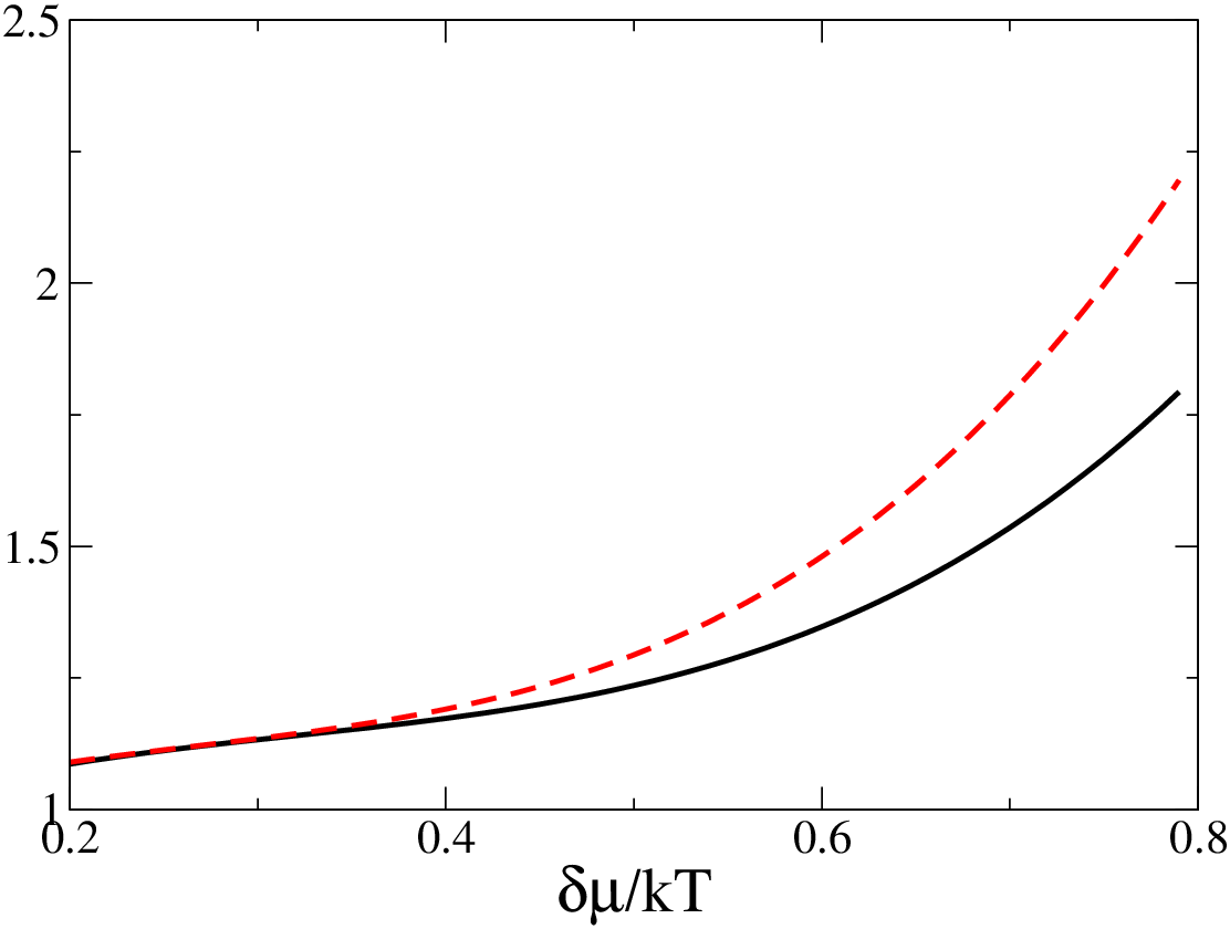
We considered the outer core radius, Eq. (48), which is obtained from an expansion around the nontrivial vacuum state . To further analyze the vortex structure, we obtain the inner core radius which uses an expansion around state, i.e. Ginsburg-Landau expansion. In C we construct the Ginsburg-Landau functional to the fourth order, and derive the equation obeyed by in a vortex configuration using the Time Dependent Ginzburg Landau equation (TDGL) [52],
| (53) |
with the boundary conditions , . The center of the vortex is at , and the expressions for the coefficients are reported in Eq. (100). Notice that the TDGL equations for the vortex configuration are valid for where the gap is vanishing small. Introducing , with a dimensionless variable, we obtain the TDGL equation for the radial part of the condensate configuration
| (54) |
with boundary conditions and , and where the expression for the coefficients , , are reported in Eq. (103). At nonzero , we solve numerically the TDGL equation for various values of . In the left panel of Fig. 6 we report the result of the numerical solution of the condensate and of its derivative for . In the right panel of Fig. 6 we report the value of the vortex radius as a function of . The two curves correspond to two different definitions of the vortex radius. based on a certain value of either the condensate or it’s derivative. Although calculations are done at nonzero , one may assume that the same trend holds for vanishing temperatures.
5 Conclusions
In conclusion, our results show that as we move into the gapless regime, the outer radius of the vortex increases sharply. This rise may be observed in experiments done with cold atomic gases trapped in a magnetic trap.
If the parameters of the trap, namely, the number of particles of the two species, and , and the scattering length, , are tuned such that there is a sufficiently wide region in position space where the atomic system is in the gapless BEC phase, this dramatic effect can be seen. We leave the precise determination of parameters , and for future work, but it will presumably require very flat traps to realize this phenomenon in a wide enough region in the system to be observed cleanly.
The properties of vortices in the gapless region have been studied previously in [58, 59] who have concentrated on the interaction between two vortices in this regime. The vortex core structure in imbalanced superfluids has been studied in [60] who have focused on the occupation number of particles that determine the “visibility" of vortices. The authors of [61] used a Bogoliubov-de Gennes approach to solve for a vortex core state in fermion mixtures with unequal masses. They found that the vortex core is mostly occupied by the light mass fermions and that the core density of the heavy-mass fermions is highly depleted. We believe that their study points towards the gapless phases, however their calculations are more involved. Our study provides motivation to study a new observable, namely the size of the core of a vortex, in the gapless phase.
Finally, we comment about the instability toward the formation of a non homogeneous phase. One can see Fig. 3 that in the strong coupling regime the coefficient is always positive. Indeed, along the curves corresponding to and in Fig. 3 the coefficient is positive and large. This means that there is no instability toward a LOFF-like phase. This is consistent with the results of Ref. [23], where the LOFF phase was found to be favored in the weak coupling regime only. Indeed from Fig. 3 one can see that in the weak coupling limit, the curves corresponding to or pass through the region where is negative and this indicates that it is possible to have a non homogeneous LOFF phase. But to really check the favorability of a LOFF-like phase in this region, in a small calculation, one should expand around the solution with and not . The reason being that the phase transition from (some) LOFF phases to the normal phase is second order and one can study how fluctuations drive the system from the homogeneous normal phase to a non homogeneous phase. We leave such an analysis for future work.
6 Acknowledgement
The authors thank Andreas Schmitt and Sanjay Reddy for their valuable comments on the manuscript. EG and RS thank Michael Forbes, Dam Son, Misha Stephanov, Eugene Demler, Bertrand Halperin, Martin Zwierlein, Leonid Levitov and Carlos Sa de Melo for discussions. RS acknowledges several discussions with Sanjay Reddy. The work of MM has been supported by the Ministerio de Educación y Ciencia (MEC) and CPAN under grants FPA2007-66665 and 2009SGR502. RS is supported by LANS, LLC for the NNSA of the DOE under contract DE-AC52-06NA25396.
Appendix A Relations between the Meissner mass, the Debye mass and the coefficients of the effective action describing the phase fluctuations
We show the equivalence between the screening masses and the coefficients in effective action for the Nambu-Goldstone mode. This equivalence can be anticipated from gauge invariance if we gauge the global symmetry associated with total number conservation [62]. The gauged action is invariant under a local rotation in the phase of the fermion fields , with , accompanied by gauge transformation on the four vector . (We apologize to the reader that we use the same Latin character for the gauge fields as well as for the operator defined in Eq. (26). They can be easily distinguished because gauge fields always appear with a subscript () or in bold font ().) The condensate in Eq. (3) spontaneously breaks this gauge symmetry, and therefore by the Anderson-Higgs mechanism, the gauge field components , acquire a Meissner screening mass. The component of the gauge field is instead Debye screened. (In the gapless regime, there is an additional contribution to the Debye mass from the fermions in the blocking regions, that we do not consider here [47]. Adding this contribution to the pairing contribution that we calculate, gives the net Debye mass square for the system.) In this Section we explicitly show that the screening masses can be related to the coefficients that appear in the effective Lagrangian describing the Nambu-Goldstone bosons.
On gauging the quadratic part of the Nambu-Gorkov action in Eq. (16) we obtain
| (55) |
A gauge transformation is given by , for fermions, leading to for the condensate, and by , for the gauge field. Since the term with is common in all the following expressions, we will stop writing it explicitly from Eq. (A) to Eq. (85) and carry it implicitly, and only write it in the final expression Eq. (86).
First we establish the coefficients in the effective action of Nambu-Goldstone mode, in the absence of any external gauge fields. These are space-time dependent phase rotations of the -field which we parameterize as . The quadratic piece of the Nambu-Gorkov fields has the form,
where and are given by Eq. (3.2). To the relevant order this phase shifts to , with fluctuations being given by . The effective action for is obtained by integrating out the fermions and can be written directly from Eq. (37) by substituting this value of . We obtain,
| (64) |
where .
Next we remove the phase from the condensate by redefining the phases of the fermionic fields. This will give rise to non-zero values of the gauge fields and we evaluate the screening masses of these gauge fields. Redefining and acting with a derivative operator, the quadratic part of the action can be written as
where is given by Eq. (3.2), and is given by
| (73) |
which includes first and second order terms in . This Lagrangian is exactly of the form given by Eq. (55) with and hence the gauge boson masses can be read from the Lagrangian describing the fields.
To show that the masses we obtain this way are the same as the coefficients obtained by treating as the Nambu-Goldstone field (Eq. (64)) we explicitly calculate the second order correction to the action using Eq. (17). We will analyze separately the quadratic term that contain only spatial derivatives of , the term that contain only time derivatives of and the mixed term.
Consider the quadratic spatial component, . Both linear and quadratic terms in contribute to this part of the effective action. Indeed from the expansion of the action we obtain
| (74) |
Note that differential operator in acts on external in- and out-going legs, i.e. produces and , while the other acts inside the loop, producing and . Using the definitions of and (Eq. (26)) the term proportional to on the right hand side of Eq. (74) simplifies to
| (75) |
The second term on the right hand side of Eq. (74) can be simplified by noticing that
| (76) |
Then the second term on the rhs of Eq. (74) is given by
| (77) | |||||
where
Here we have used Eq. (76) to rewrite the combination and to extract extra power of and in the numerator. Combining all the terms together, we get for the spatial component of the effective action
| (78) |
Now we turn to the quadratic term containing only temporal derivatives, i.e. . Only terms quadratic in contribute to this part of the effective action (Eq. (17)),
| (79) |
We can simplify this expression, noticing that one can write
| (80) |
whereupon the right hand side of Eq. (79) can be rewritten as
| (81) |
where,
| (82) |
Then, the term of the effective action containing the temporal derivatives of turns out to be given by
| (83) |
Finally we consider the mixed component, . The only contribution to this part of the action comes from the quadratic term in (Eq. (17)). Therefore,
| (84) |
We use Eq. (76) to simplify the mixed term, and we obtain the following contribution to the effective action
| (85) |
The sum of the three terms, Eq. (78),(83) and (85), gives the effective action for the gauge field
| (86) |
We recognize that by putting in we reproduce the Meissner mass, and by putting , i.e. , we obtain the Debye mass. Comparing Eq. (64) and Eq. (86), we see that coefficients in the effective action for the Nambu-Goldstone mode coincide with the corresponding screening masses as we set out to show.
Appendix B Coefficients of the low energy Lagrangian
The sum over the Matsubara frequencies can be done analytically noticing that if is a function with no poles then one has
| (87) |
for . Upon substituting this result in Eq. (30) one obtains the usual form of the gap equation at non vanishing temperatures:
| (88) |
where for infinite volume, the sum over can be replaced by an integral over three-momentum and where we have defined,
with the Fermi-Dirac distribution function.
After evaluating the Matsubara sums using Eq. (87), we get the following expressions,
| (89) | |||||
where the sum is an integral over the three-momentum and we have indicated with and the quantities and respectively, with and the quantities and respectively, and where .
The expressions of the coefficients , , , , and in Eq.(38) are given by
| (90) |
where refers to the differentiation of with respect to .
To evaluate the integrals we use the following relations. For any function we have,
| (91) | |||||
where , and . In Eq. (91), all algebraic terms featuring appear with a corresponding product of functions, , which we have omitted for clarity. Whenever appear as limits of the integrals, we can simply use the definitions of given above to obtain the correct answer.
We analyze the values of the coefficients at . This can be done by taking the limit in Eq. (90). We obtain the following expressions:
| (92) |
The equation for is more complicated and hence we do not give the detailed final expression which however can be obtained from the following equation:
| (93) | |||||
where,
| (94) |
For completeness we give the expression for which can be evaluated similarly,
| (95) |
Appendix C TDGL equation for the vortex core states
To analyze the vortex core structure we derive the Ginsburg-Landau functional expanding the action
| (96) |
around a state with up to the fourth order in , obtaining
where are defined in Eq. (26). We rewrite the action as
| (97) |
where can be written as
| (98) |
We perform the Matsubara sum, take , the limit and obtain the effective action
| (99) |
where the coefficients are given by
| (100) |
where , is the Fermi distribution, , , , and we take . The equation of motion, , is given by
| (101) |
and in configuration space
| (102) |
with the boundary conditions , . At , we have
| (103) | |||||
where we introduced , and the dimensionless variables , and ; zeros of the quasiparticle energy are at .
Introducing with dimensionless , we obtain the TDGL equation for the vortex core at
| (104) |
with boundary conditions and . The coefficients , , are given in the right hand side of Eq. (103). Coefficients correspond to a superfluid ideal Bose gas discussed by Landau [63], where a vortex filament has macroscopic thickness. Here we are able to study both regimes of BCS and BEC, BCS-BEC transition, as well as the situation with nonzero mismatch, . We solve this second order ODE numerically for different values of .
References
- [1] M. W. Zwierlein, A. Schirotzek, C. H. Schunck, and W. Ketterle, Science 311, 492 (2006) [arXiv:cond-mat/0511197]; M. W. Zwierlein and W. Ketterle, arXiv:cond-mat/0603489; Y.-Il Shin, C. H. Schunck, A. Schirotzek and W. Ketterle, arXiv:0709.3027.
- [2] G. B. Partridge, W. Li, R. I. Kamar, Y.-a. Liao, and R. G. Hulet, Science 311, 503 (2006) [arXiv:cond-mat/0511752].
- [3] B. S. Chandrasekhar, Appl. Phys. Lett. 1, 7 (1962); A. M. Clogston, Phys. Rev. Lett. 9, 266 (1962).
- [4] G. Sarma, Phys. Chem. Solids 24, 1029 (1963).
- [5] P. Fulde and R. A. Ferrell, Phys. Rev. 135, A550 (1964); A. I. Larkin and Y. N. Ovchinnikov, Sov. Phys. JETP 20, 762 (1965).
- [6] H. Muther and A. Sedrakian, Phys. Rev. Lett. 88, 252503 (2002) [arXiv:cond-mat/0202409].
- [7] P. F. Bedaque, H. Caldas and G. Rupak, Phys. Rev. Lett. 91, 247002 (2003) [arXiv:cond-mat/0306694].
- [8] W. V. Liu and F. Wilczek, Phys. Rev. Lett. 90 (2003) 047002 [arXiv:cond-mat/0208052].
- [9] E. Gubankova, W. V. Liu and F. Wilczek, Phys. Rev. Lett. 91 (2003) 032001 [arXiv:hep-ph/0304016].
- [10] M. M. Forbes, E. Gubankova, W. V. Liu and F. Wilczek, Phys. Rev. Lett. 94, 017001 (2005) [arXiv:hep-ph/0405059].
- [11] J. Carlson and S. Reddy, Phys. Rev. Lett. 95, 060401 (2005) [arXiv:cond-mat/0503256].
- [12] P. Castorina, M. Grasso, M. Oertel, M. Urban and D. Zappala, Phys. Rev. A 72 (2005) 025601 [arXiv:cond-mat/0504391].
- [13] C. H. Pao, S.-T. Wu, and S. K. Yip, Phys. Rev. B 73, 132506 (2006) [arXiv:cond-mat/0506437].
- [14] C. H. Pao, S.-T. Wu, and S. K. Yip, [arXiv:cond-mat/0608501].
- [15] D. T. Son and M. A. Stephanov, Phys. Rev. A 74, 013614 (2006) [arXiv:cond-mat/0507586].
- [16] D. E. Sheehy and L. Radzihovsky, Phys. Rev. Lett. 96, 060401 (2006) [arXiv:cond-mat/0508430]; Annals of Physics, 322, 1790, 2007 [arXiv:cond-mat/0607803v2]; Phys. Rev. B 75, 136501 (2007) [arXiv:cond-mat/0608172].
- [17] K. Yang, arXiv:cond-mat/0508484.
- [18] P. Pieri and G. C. Strinati, Phys. Rev. Lett. 96, 150404 (2006), [arXiv:cond-mat/0512354]; J. Kinnunen, L. M. Jensen and P. Torma Phys. Rev. Lett. 96, 110403 (2006) [arXiv:cond-mat/0512556]; W. Yi and L.-M. Duan, Phys. Rev. A 73, 031604(R) (2006) [arXiv:cond-mat/0601006]; F. Chevy, arXiv:cond-mat/0601122; T. N. De Silva, E. J. Mueller, Phys. Rev. A 73, 051602(R) (2006) [arXiv:cond-mat/0601314]; M. Haque and H. T. C. Stoof, Phys. Rev. A 74, 011602 (2006) [arXiv:cond-mat/0601321]; C. H. Pao and S. K. Yip, J. Phys. Condens. Matter 18 5567 (2006) [arXiv:cond-mat/0604530]; M. M. Parish, F. M. Marchetti, A. Lamacraft and B. D. Simons, Phys. Rev. Lett. 98 160402 (2007) [arXiv:cond-mat/0608651]; For a recent review on the properties of trapped fermi gases, and more references, see S. Giorgini, L. P. Pitaevskii and S. Stringari, arXiv:0706.3360v2.
- [19] Q. Chen, J. Stajic, S. Tan and K. Levin, Phys. Rep. 412,1 (2005).
- [20] A. Bulgac, M. M. Forbes and A. Schwenk, arXiv:cond-mat/0602274.
- [21] K. Yang, arXiv:cond-mat/0603190.
- [22] E. Gubankova, A. Schmitt and F. Wilczek, arXiv:cond-mat/0603603.
- [23] M. Mannarelli, G. Nardulli and M. Ruggieri, Phys. Rev. A 74, 033606 (2006) arXiv:cond-mat/0604579.
- [24] J. Carlson and S. Reddy arXiv:cond-mat/0711.0414.
- [25] E. Tiesinga, B. J. Verhaar abd H. T. C. Stoof, Phys. Rev. A 47, 4114 (1993); S. Inouye et al., Nature 392, 151 (1998); P. Courteille et al., Phys. Rev. Lett. 81, 69 (2004); J. L. Roberts et al., Phys. Rev. Lett. 81, 5109 (1998); E. Timmermans, P. Tommasini, M. Hussein and A. Kerman, Phys. Rep. 315, 199 (1999).
- [26] D. M. Eagles, Phys. Rev. 186, 456 (1969); A. J. Leggett in Modern Trends in the theory of condensed matter, edited by A. Pekalski and J. Przystawa (Springer-Verlag, Berlin, 1980).
- [27] M. Y. Veillette, D. E. Sheehy and L. Radzihovsky, Phys. Rev. A 75, 043614 (2007).
- [28] R. B. Diener, R. Sensarma and M. Randeria, arXiv:0709.2653.
- [29] Y. Nishida and D. T. Son, Phys. Rev. Lett. 97, 050403 (2006) [arXiv:cond-mat/0604500]; Y. Nishida and D. T. Son, Phys. Rev. A 75, 063617 (2007), [arXiv:cond-mat/0607835].
- [30] R. Casalbuoni and G. Nardulli, Rev. Mod. Phys. 76, 263 (2004) [arXiv:hep-ph/0305069].
- [31] K. Yang, arXiv:cond-mat/0603190.
- [32] L. He, M. Jin and P. Zhuang, Phys. Rev. B 73, 214527 (2006).
- [33] Z. Nussinov and S. Nussinov, Phys. Rev. A 74, 053622 (2006) [arXiv:cond-mat/0410597].
- [34] P. Nikolic and S. Sachdev, Phys. Rev. A 75, 033608 (2007).
- [35] A. Bulgac and M. M. Forbes, Phys. Rev. A 75, 031605 (2007) [arXiv:cond-mat/0606043].
- [36] A. Bulgac, arXiv:cond-mat/0703526.
- [37] J. R. Engelbrecht, M. Randeria, and C. A. R. Sá de Melo, Phys. Rev. B 55, 15153 (1997).
- [38] F. Dalfovo, S. Giorgini, L. P. Pitaevskii and S. Stringari, Rev. Mod. Phys. 71, 463 (1999).
- [39] R. Combescot, M. Y. Kagan and S. Stringari, Phys. Rev. A 74, 042717 (2006) [arXiv:cond-mat/0607493].
- [40] A. M. J. Schakel, [arxiv:0912.1955].
- [41] M. Marini, F. Pistolesi and G. C. Strinati Eur. Phys. J B1, 151 (1998) [arXiv:cond-mat/9703160].
- [42] G. Rupak and T. Schafer, arXiv:0707.1520 [cond-mat.other].
- [43] A. Kryjevski, arXiv:0712.2093 [nucl-th].
- [44] M. Huang and I. A. Shovkovy, Phys. Rev. D 70, 051501 (2004) [arXiv:hep-ph/0407049]; M. Huang and I. A. Shovkovy, Phys. Rev. D 70, 094030 (2004) [arXiv:hep-ph/0408268]; I. Giannakis and H. C. Ren, Phys. Lett. B 611, 137 (2005) [arXiv:hep-ph/0412015]; M. Alford and Q. h. Wang, J. Phys. G 31, 719 (2005) [arXiv:hep-ph/0501078]; M. Huang, Phys. Rev. D 73, 045007 (2006) [arXiv:hep-ph/0504235]; E. V. Gorbar, M. Hashimoto and V. A. Miransky, Phys. Lett. B 632, 305 (2006) [arXiv:hep-ph/0507303]; E. V. Gorbar, M. Hashimoto, V. A. Miransky and I. A. Shovkovy, Phys. Rev. D 73, 111502 (2006) [arXiv:hep-ph/0602251]; K. Iida and K. Fukushima, Phys. Rev. D 74, 074020 (2006) [arXiv:hep-ph/0603179].
- [45] R. Casalbuoni, R. Gatto, M. Mannarelli, G. Nardulli and M. Ruggieri, Phys. Lett. B 605, 362 (2005) [Erratum-ibid. B 615, 297 (2005)] [arXiv:hep-ph/0410401]; K. Fukushima, Phys. Rev. D 72, 074002 (2005) [arXiv:hep-ph/0506080].
- [46] K. Fukushima, Phys. Rev. D 73, 094016 (2006) [arXiv:hep-ph/0603216].
- [47] R. Gatto and M. Ruggieri, Phys. Rev. D 75, 114004 (2007) [arXiv:hep-ph/0703276].
- [48] I. Giannakis, D. Hou, M. Huang and H. c. Ren, Phys. Rev. D 75, 014015 (2007) [arXiv:hep-ph/0609098].
- [49] I. Giannakis, D. Hou, M. Huang and H. c. Ren, Phys. Rev. D 75, 011501 (2007) [arXiv:hep-ph/0606178].
- [50] T. N. De Silva and E. J. Mueller, Phys. Rev. Lett. 97, 070402 (2006) [arXiv:cond-mat/0604638].
- [51] A. Lamacraft and F. M. Marchetti, Phys. Rev. B 77, 014511 (2008) [arXiv:cond-mat/0701692].
- [52] C. A. R. Sá de Melo, M. Randeria, and J. R. Engelbrecht, Phys. Rev. Lett. 71, 3202 (1993).
- [53] M. Mannarelli, K. Rajagopal and R. Sharma, Phys. Rev. D 76, 074026 (2007) [arXiv:hep-ph/0702021]; M. Mannarelli, K. Rajagopal and R. Sharma, AIP Conf. Proc. 964, 264 (2007) [arXiv:0710.0331 [hep-ph]].
- [54] J. I. Kapusta, Finite Temperature Field Theory (Cambridge University Press, Cambridge, England, 1989).
- [55] M. G. Alford, M. Braby and A. Schmitt, J. Phys. G 35, 025002 (2008) [arXiv:0707.2389 [nucl-th]].
- [56] An expansion of the effective action that includes terms of order has been done in [16]. Since the coefficient of the term vanishes in the gapless region this will probably lead to a vortex core that is even larger than the one we have estimated.
- [57] C. F. Barenghi, R. J. Donelly and W. F. Vinen, Jouranl of Low Temperature Physics, 52, 189 (1983)
- [58] V. M. Stojanovic, W. V. Liu and Y. B. Kim, [arXiv:cond-mat/0611295].
- [59] V. M. Stojanovic, W. V. Liu and Y. B. Kim, Annals of Physics, 323, 989, 2008, [arXiv:0710.2522 [cond-mat]].
- [60] M. Takahashi, T. Mizushima, M. Ichioka, and K. Machida, Phys. Rev. Lett. 97, 180407 (2006).
- [61] M. Iskin, Phys. Rev. A 78, 021604(R) (2008); [arXiv:con-mat/0804.1035]; arXiv:cond-mat/0810.5065.
- [62] D. T. Son and M. A. Stephanov, Phys. Rev. D 61, 074012 (2000) [arXiv:hep-ph/9910491].
- [63] L. D. Landau, E. M. Lifshitz, "Fluid Mechanics" (2nd ed), Chapter 30 “A vortex filament in an almost ideal bose gas", (see original refs. there V. L. Ginzburg and L. P. Pitaevskii (1958); L. P. Pitaevskii (1961); E. P. Gross (1961)).