跳到论文正文
W Papers独立论文阅读器 arXiv:0804.0780 论文正文 计算阅读时间 · 0%
引用这篇论文根据当前论文元数据生成,正式投稿前建议核对。


License: arXiv.org perpetual non-exclusive license
arXiv:0804.0780v2 [math.DS] 04 Apr 2008

Renormalization in the Hénon family, II:
The heteroclinic web

M. Lyubich, M. Martens Address: Stony Brook University and University of Toronto
Date: August 24, 2026
Abstract.

We study highly dissipative Hénon maps

Fc,b:(x,y)↦(c−x2−b​y,x)F_{c,b}:(x,y)\mapsto(c-x^{2}-by,x)

with zero entropy. They form a region Π\Pi in the parameter plane bounded on the left by the curve WW of infinitely renormalizable maps. We prove that Morse-Smale maps are dense in Π\Pi, but there exist infinitely many different topological types of such maps (even away from WW). We also prove that in the infinitely renormalizable case, the average Jacobian bFb_{F} on the attracting Cantor set 𝒪F{\mathcal{O}}_{F} is a topological invariant. These results come from the analysis of the heteroclinic web of the saddle periodic points based on the renormalization theory. Along these lines, we show that the unstable manifolds of the periodic points form a lamination outside 𝒪F{\mathcal{O}}_{F} if and only if there are no heteroclinic tangencies.

Stony Brook IMS Preprint #2008/2 April 2008

1. Introduction

The renormalization theory for the Hénon family began with the works of Collet, Eckman and Koch and Gambaudo, van Strien and Tresser [CEK], [GST]. In this paper we continue our exploration of renormalization of Hénon maps started in [CLM]. As Part I was mostly concerned with geometric properties of the Cantor attractor 𝒪F{\mathcal{O}}_{F}, here we focus on global topological properties of the maps in question that are essentially determined by the structure of the web of the stable/unstable manifolds of saddle periodic points (we call it the “heteroclinic web”). As in Part I, we have encountered here some surprising phenomena.

In the one-dimensional situation, all infinitely renormalizable maps with the same combinatorics are topologically equivalent. It is not anymore the case in the Hénon family; in fact, all infinitely renormalizable Hénon maps near the Feigenbaum point are topologically distinct. More generally, the average Jacobian bFb_{F} of a Hénon-like map is a topological invariant: varying bFb_{F} leads to bifurcations in the heteroclinic web (§9).

Along these lines, we carry out a detailed analysis of the heteroclinic web. In particular, we show that the unstable manifolds form a lamination (outside the attractor 𝒪F{\mathcal{O}}_{F}) if and only if there are no heteroclinic tangencies (§§4,6). We also show that the orbit of the “tip” of 𝒪F{\mathcal{O}}_{F} (a counterpart of the critical value of one-dimensional maps) is topologically distinguished: it is respected by topological conjugacies (§5).

Refer to caption
Figure 1.1. Bifurcation pattern

Infinitely renormalizable maps in question separate the regions with regular (zero entropy) and chaotic (positive entropy) dynamics, [GST]. Because of the Newhouse phenomenon, hyperbolic maps are not dense in the chaotic region. However, it is conceivable that they are dense in the regular region. We confirm this conjecture in a narrow strip to the left of the curve of infinitely renormalizable maps: Morse-Smale maps are dense over there (§10). However, the situation is quite intricate, as there are infinitely many different types of Morse-Smale maps in this region. In particular, a boundary arc of a Morse-Smale component which is not related to the longest periodic orbit is accumulated by infinitely many different Morse-Smale components.

Remark 1.1.

The maps in the region we consider, a narrow strip to the left of the curve of infinitely renormalizable maps, do not have homoclinic intersections. Previous results in [PS] and [C] imply that maps in this region can be C1C^{1} approximated by Morse-Smale maps.

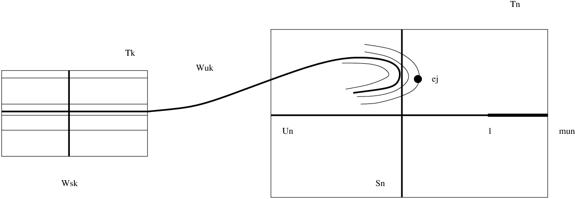
The results of §10 are illustrated in Figure 1.1. It shows an artist’s impression of parts of the bifurcation pattern of a Hénon family in a neighborhood of WW, the curve of infinitely renormalizable maps. The strip ImI_{m} consists of the mm-times renormalizable maps. The bottom Morse-Smale component MmM_{m} is attached to the mm-times renormalizable unimodal maps. The curves 𝒦⋅,⋅{\mathcal{K}}_{\cdot,\cdot} illustrate loci of heteroclinic tangencies.

Acknowledgements

We thank Andre de Carvalho and Charles Tresser for many inspiring Hénon discussions. We also thank all the institutions and foundations that have supported us in the course of this work: Simons Mathematics and Physics Endowment, Fields Institute, NSF, NSERC, University of Toronto.

2. Preliminaries

The precise definitions and proofs of the following statements can be found in part I, see [CLM], of this series on renormalization of Hénon maps.

Let Ωh,Ωv⊂ℂ\Omega^{h},\Omega^{v}\subset\mathbb{C} be neighborhoods of [−1,1]⊂ℝ[-1,1]\subset\mathbb{R} and Ω=Ωh×Ωv\Omega=\Omega^{h}\times\Omega^{v}. Let B=[−1,1]×[−1,1]B=[-1,1]\times[-1,1] and ϵ¯>0\overline{\epsilon}>0. The set ℋΩ​(ϵ¯){\mathcal{H}}_{\Omega}(\overline{\epsilon}) consists of maps F:B→BF:B\to B of the following form.

F⁡(x,y)=(f⁡(x)−ϵ⁡(x,y),x),F(x,y)=(f(x)-\epsilon(x,y),x),

where f:[−1,1]→[−1,1]f:[-1,1]\to[-1,1] is a unimodal map which admits a holomorphic extension to Ωh\Omega^{h} and ϵ:B→ℝ\epsilon:B\to\mathbb{R} admits a holomorphic extension to Ω\Omega and finally, |ϵ|≤ϵ¯|\epsilon|\leq\overline{\epsilon}. The critical point cc of ff is non degenerate, D​f​(c)<0Df(c)<0. A map in ℋΩ​(ϵ¯){\mathcal{H}}_{\Omega}(\overline{\epsilon}) is called a Hénon-like map. Observe that Hénon-like maps map vertical lines to horizontal lines.

A unimodal map f:[−1,1]→[−1,1]f:[-1,1]\to[-1,1] with critical point c∈[−1,1]c\in[-1,1] is renormalizable if f2:[f2​(c),f4​(c)]→[f2​(c),f4​(c)]f^{2}:[f^{2}(c),f^{4}(c)]\to[f^{2}(c),f^{4}(c)] is unimodal and [f2​(c),f4​(c)]∩f⁡([f2​(c),f4​(c)])=∅[f^{2}(c),f^{4}(c)]\cap f([f^{2}(c),f^{4}(c)])=\emptyset. The renormalization of ff is the affine rescaling of f2|([f2​(c),f4​(c)]CLOSEf^{2}|([f^{2}(c),f^{4}(c)], denoted by R​fRf. The domain of R​fRf is again [−1,1][-1,1]. The renormalization operator RR has a unique fixed point f∗:[−1,1]→[−1,1]f_{*}:[-1,1]\to[-1,1]. The introduction of [FMP] presents the history of renormalization of unimodal maps and describes the main results.

The scaling factor of this fixed point f∗f_{*} is

σ=|[f∗2​(c),f∗4​(c)]||[−1,1]|.\sigma=\frac{|[f_{*}^{2}(c),f_{*}^{4}(c)]|}{|[-1,1]|}.

We will also need λ=1/σ=2.6​…\lambda=1/\sigma=2.6\dots.

A Hénon map is renormalizable if there exists a domain D⊂BD\subset B such that F2:D→DF^{2}:D\to D. The construction of the domain DD is inspired by renormalization of unimodal maps. In particular, it is a topological construction. However, for small ϵ¯>0\overline{\epsilon}>0 the actual domain A⊂BA\subset B, used to renormalize as was done in [CLM], has an analytical definition. The precise definition can be found in §3.5 of part I. If the renormalizable Hénon maps is given by F⁡(x,y)=(f⁡(x)−ϵ⁡(x,y))F(x,y)=(f(x)-\epsilon(x,y)) then the domain A⊂BA\subset B, an essentially vertical strip, is bounded by two curves of the form

f⁡(x)−ϵ⁡(x,y)=Const.f(x)-\epsilon(x,y)=\text{Const}.

These curves are graphs over the yy-axis with a slope of the order ϵ¯>0\overline{\epsilon}>0. The domain AA satisfies similar combinatorial properties as the domain of renormalization of a unimodal map:

F⁡(A)∩A=∅,F(A)\cap A=\emptyset,

and

F2​(A)⊂A.F^{2}(A)\subset A.

Unfortunately, the restriction F2|AF^{2}|A is not a Hénon-like map as it does not map vertical lines into horizontal lines. This is the reason why the coordinated change needed to define the renormalization of FF is not an affine map, but it rather has the following form. Let

OPENH⁡(x,y)=(f⁡(x))−ϵ⁡(x,y),y)H(x,y)=(f(x))-\epsilon(x,y),y)

and

G=H∘F2∘H−1.G=H\circ F^{2}\circ H^{-1}.

The map HH preserves horizontal lines and it is designed in such a way that the map GG maps vertical lines into horizontal lines. Moreover, GG is well defined on a rectangle U×[−1,1]U\times[-1,1] of full height. Here U⊂[−1,1]U\subset[-1,1] is an interval of length 2/|s|2/|s| with s<−1s<-1. Let us rescale the domain of GG by the ss-dilation Λ\Lambda, such that the rescaled domain is of the form [−1,1]×V[-1,1]\times V, where V⊂ℝV\subset\mathbb{R} is an interval of length 2/|s|2/|s|. Define the renormalization of FF by

R​F=Λ∘G∘Λ−1.RF=\Lambda\circ G\circ\Lambda^{-1}.

Notice that R​FRF is well defined on the rectangle [−1,1]×V[-1,1]\times V. The coordinate change ϕ=H−1∘Λ−1\phi=H^{-1}\circ{\Lambda}^{-1} maps this rectangle onto the topological rectangle AA of full height.

The set of nn-times renormalizable maps is denoted by ℋΩn​(ϵ¯)⊂ℋΩ​(ϵ¯){\mathcal{H}}^{n}_{\Omega}(\overline{\epsilon})\subset{\mathcal{H}}_{\Omega}(\overline{\epsilon}). If F∈ℋΩn​(ϵ¯)F\in{\mathcal{H}}^{n}_{\Omega}(\overline{\epsilon}) we use the notation

Fn=Rn​F.F_{n}=R^{n}F.

The set of infinitely renormalizable maps is denoted by

ℐΩ​(ϵ¯)=⋂n≥1ℋΩn​(ϵ¯).{\mathcal{I}}_{\Omega}(\overline{\epsilon})=\bigcap_{n\geq 1}{\mathcal{H}}^{n}_{\Omega}(\overline{\epsilon}).

The collection of maps in ℋΩn​(ϵ¯){\mathcal{H}}^{n}_{\Omega}(\overline{\epsilon}) which have a periodic attractor of period 2n2^{n} is denoted by ℐΩn​(ϵ¯){\mathcal{I}}^{n}_{\Omega}(\overline{\epsilon}).

The renormalization operator acting on ℋΩ1​(ϵ¯){\mathcal{H}}^{1}_{\Omega}(\overline{\epsilon}), ϵ¯>0\overline{\epsilon}>0 small enough, has a unique fixed point F∗∈ℐΩ​(ϵ¯)F_{*}\in{\mathcal{I}}_{\Omega}(\overline{\epsilon}). It is the degenerate map

F∗​(x,y)=(f∗​(x),x).F_{*}(x,y)=(f_{*}(x),x).

This renormalization fixed point is hyperbolic and the stable manifold has codimension one. Moreover,

Ws​(F∗)=ℐΩ​(ϵ¯).W^{s}(F_{*})={\mathcal{I}}_{\Omega}(\overline{\epsilon}).

If we want to emphasize that some set, say AA, is associated with a certain map FF we use notation like A⁡(F)A(F).

The coordinate change which conjugates Fk2|A⁡(Fk)F_{k}^{2}|A(F_{k}) to Fk+1F_{k+1} is denoted by

(2.1) ϕvk=(Λk∘Hk)−1:Dom⁡(Fk+1)→A⁡(Fk).\phi^{k}_{v}=(\Lambda_{k}\circ H_{k})^{-1}:\operatorname{Dom}(F_{k+1})\to A(F_{k}).

Here HkH_{k} is the non-affine part of the coordinate change used to define Rk+1​FR^{k+1}F and Λk\Lambda_{k} is the dilation by sk<−1s_{k}<-1. Now, for k<nk<n, let

(2.2) Φkn=ϕvk∘ϕvk+1∘⋯∘ϕvn−1:Dom(Fn)→An−k(Fk),\Phi^{n}_{k}=\phi^{k}_{v}\circ\phi^{k+1}_{v}\circ\cdots\circ\phi^{n-1}_{v}:\operatorname{Dom}(F_{n})\to A_{n-k}(F_{k}),

where

Ak​(F)=Φ0k​(Dom⁡(Fk))∩B.A_{k}(F)=\Phi^{k}_{0}(\operatorname{Dom}(F_{k}))\cap B.

Notice, that each Ak⊂BA_{k}\subset B is of full height and Φ0k\Phi^{k}_{0} conjugates Rk​FR^{k}F to F2k|AkF^{2^{k}}|A_{k}. Furthermore, Ak+1⊂AkA_{k+1}\subset A_{k}.

Let n≥1n\geq 1 and F∈ℋΩn​(ϵ¯)F\in{\mathcal{H}}^{n}_{\Omega}(\overline{\epsilon}). The domain of Rn​FR^{n}F is

Ωn=Ωnh×Ωnv,\Omega_{n}=\Omega^{h}_{n}\times\Omega^{v}_{n},

where [−1,1]⊂Ωnh[-1,1]\subset\Omega^{h}_{n}. Furthermore, Rn​F​(x,y)=(fn​(x)−ϵn​(x,y),x)R^{n}F(x,y)=(f_{n}(x)-\epsilon_{n}(x,y),x).

Lemma 2.1.

Given Ω\Omega and ϵ¯>0\overline{\epsilon}>0 small enough, there exist r>1r>1 and C>0C>0 such that for every F∈ℋΩn​(ϵ¯)F\in{\mathcal{H}}^{n}_{\Omega}(\overline{\epsilon})

diam⁡(Ωn)≤C⋅rn.\operatorname{diam}(\Omega_{n})\leq C\cdot r^{n}.
Proof.

Let k<nk<n. The maps fk|Ωkhf_{k}|\Omega^{h}_{k} stay within a compact family and |ϵk|=O⁡(ϵ¯2k)|\epsilon_{k}|=O(\overline{\epsilon}^{2^{k}}). This is explained in §4 of [CLM]. Hence, the coordinate changes Λk∘Hk\Lambda_{k}\circ H_{k} used to define Rk+1​FR^{k+1}F as a renormalization of Rk​FR^{k}F has a uniform bound on its derivative. The Lemma follows. ∎

Remark 2.1.

For an infinitely renormalizable map F∈ℐΩ​(ϵ¯)F\in{\mathcal{I}}_{\Omega}(\overline{\epsilon}) the diameters of Ωn\Omega_{n} grow exponentially. In particular

diam⁡(Ωnv)≍λn,\operatorname{diam}(\Omega^{v}_{n})\asymp\lambda^{n},

where λ=1/σ=2.6​…\lambda=1/\sigma=2.6\dots and σ\sigma the scaling factor of the unimodal renormalization fixed point. Let Φkk+1:Ωk+1→Ωk\Phi^{k+1}_{k}:\Omega_{k+1}\to\Omega_{k} be the diffeomorphism which conjugates Rk+1​FR^{k+1}F to (Rk​F)2|A⁡(Rk​F)(R^{k}F)^{2}|A(R^{k}F). The inverse of this diffeomorphism was constructed in §3.5 of [CLM]. In fact,

(Φkk+1)−1=Λk∘Hk,(\Phi^{k+1}_{k})^{-1}=\Lambda_{k}\circ H_{k},

where Hk​(x,y)=(fk​(x)−ϵk​(x,y),y)H_{k}(x,y)=(f_{k}(x)-\epsilon_{k}(x,y),y) and Λk\Lambda_{k} is a dilation. The scaling factor sks_{k} of Λk\Lambda_{k} converges exponentially fast: sk→−λs_{k}\to-\lambda. This is shown in Lemma 7.4 of [CLM]. In particular,

diam⁡(Ωk+1v)=|sk|⋅diam⁡(Ωkv).\operatorname{diam}(\Omega^{v}_{k+1})=|s_{k}|\cdot\operatorname{diam}(\Omega^{v}_{k}).

Let

Bvn=Φ0n​(B).B_{v^{n}}=\Phi^{n}_{0}(B).

Notice, for k<nk<n

Bvk+1⊂Bvk.B_{v^{k+1}}\subset B_{v^{k}}.

An infinitely renormalizable Hénon-like map has an invariant Cantor set:

𝒪F=⋂n≥1⋃i=02n−1Fi​(Bvn).{\mathcal{O}}_{F}=\bigcap_{n\geq 1}\bigcup_{i=0}^{2^{n}-1}F^{i}(B_{v^{n}}).

Its geometry was discussed in part I. The dynamics on this Cantor set is conjugate to an adding machine. Its unique invariant measure is denoted by μ\mu. The average Jacobian

bF=exp∫logJacFdμb_{F}=\exp\int\log\operatorname{Jac}Fd\mu

with respect to μ\mu is an important parameter that essentially influences the geometry of 𝒪F{\mathcal{O}}_{F}, see [CLM].

The critical point (and critical value) of a unimodal map plays a crucial role in its dynamics. The counterpart of the critical value for Hénon-like maps is the tip

{τF}=⋂n≥1Bvn.\{\tau_{F}\}=\bigcap_{n\geq 1}B_{v^{n}}.

The convergence Rn​F→F∗R^{n}F\to F_{*} is exponential, F∈ℐΩ​(ϵ¯)F\in{\mathcal{I}}_{\Omega}(\overline{\epsilon}). Theorem 7.9 of [CLM] gives a precise asymptotical form of the convergence. Namely,

(2.3) Rn​F​(x,y)=(fn​(x)−bF2n​a​(x)​y​(1+O⁡(ρn)),x).R^{n}F(x,y)=(f_{n}(x)-b_{F}^{2^{n}}a(x)y(1+O(\rho^{n})),x).

The analytic function a⁡(x)a(x) is universal, independent of FF, and positive, and ρ<1\rho<1. The unimodal part converges exponentially fast: fn→f∗f_{n}\to f_{*}.

We will use the following general notions and notations throughout the text.

A ball in a metric space of radius r>0r>0 and centered at xx is denoted by Br​(x)B_{r}(x). The diameter of a set is denoted by diam​(⋅)\text{diam}(\cdot). Let π1:X×Y→X\pi_{1}:X\times Y\to X and π2:X×Y→Y\pi_{2}:X\times Y\to Y be the projections to resp. the first and second factor.

The graph of a function ϕ:X→Y\phi:X\to Y is denoted by graph​(ϕ)\text{graph}(\phi). The domain of a map FF is denoted by Dom⁡(F)\operatorname{Dom}(F). The image is denoted by Im⁡(F)=F⁡(Dom⁡(F))\operatorname{Im}(F)=F(\operatorname{Dom}(F)).

The tangent space at a point x∈Wx\in W of a smooth curve W⊂ℝ2W\subset\mathbb{R}^{2} is denoted by Tx​WT_{x}W. If two submanifolds M1M_{1} and M2M_{2} (of MM) are tangent at some point we write

M1​−⁣−∩M2.M_{1}\kern 6.99997pt\makebox[0.0pt][c]{\raisebox{3.31528pt}{$--$}}\kern-6.00006pt\cap M_{2}.

If we want to specify a point of tangency x∈M1∩M2x\in M_{1}\cap M_{2} we write

M1−⁣−∩xM2.M_{1}\kern 6.99997pt\makebox[0.0pt][c]{\raisebox{3.31528pt}{$--$}}\kern-6.00006pt\cap_{x}M_{2}.

The forward orbit of a point or set is denoted by Orb​(⋅)=⋃k≥0fk​(⋅)\text{Orb}(\cdot)=\bigcup_{k\geq 0}f^{k}(\cdot). If a point has also a complete backward orbit then the backward and forward orbit together is denoted by ○ℤ(⋅)\text{$\mathchar 525$}_{\mathbb{Z}}(\cdot). The limit set of a point x∈Dom⁡(F)x\in\operatorname{Dom}(F) is denoted by ω⁡(x)\omega(x). If a point x∈Dom⁡(F)x\in\operatorname{Dom}(F) has an infinite backward orbit then the limit set of this backward orbit is denoted by α⁡(x)\alpha(x). The cycle of a periodic point β\beta, γ\gamma etc. will be called 𝜷\beta, 𝜸{\boldsymbol{\gamma}} etc. The set of periodic points of a map FF is denoted by 𝒫F{\mathcal{P}}_{F}. A point x∈Bx\in B is a wandering point for F:B→BF:B\to B if there is a neighborhood x∈Ux\in U such that Fn​(U)∩U=∅F^{n}(U)\cap U=\emptyset, for n≥1n\geq 1. Denote the set of non-wandering points of FF by ΩF\Omega_{F}. Given two points z,z′∈Wu/s​(x)⊂Bz,z^{\prime}\in W^{u/s}(x)\subset B in the same connected component of Wu/s​(x)W^{u/s}(x), then the arc in Wu/s​(x)W^{u/s}(x) which connects zz with z′z^{\prime} is denoted by [z,z′]u/s[z,z^{\prime}]^{u/s}. When end points of such an arc are deleted we will denoted the remaining arc by (z,z′]u/s(z,z^{\prime}]^{u/s}, (z,z′)u/s(z,z^{\prime})^{u/s}, etc.

Q1≍Q2Q_{1}\asymp Q_{2} means that C−1≤Q1/Q2≤CC^{-1}\leq Q_{1}/Q_{2}\leq C, where C>0C>0 is an absolute constant or depending on, say FF.

For the reader’s convenience, more special notations are collected in the Nomenclature.

3. Local stable manifolds

Lemma 3.1.

Let U,U′,V′⊂ΩhU,U^{\prime},V^{\prime}\subset\Omega_{h} with U′¯⊂V′\overline{U^{\prime}}\subset V^{\prime}. Assume, U′⊂ΩvU^{\prime}\subset\Omega^{v}. There exists C>0C>0 such that the following holds. If F∈ℋΩ​(ϵ¯)F\in{\mathcal{H}}_{\Omega}(\overline{\epsilon}), F⁡(x,y)=(f⁡(x)−ϵ⁡(x,y),x)F(x,y)=(f(x)-\epsilon(x,y),x), and f:V′→f⁡(V′)f:V^{\prime}\to f(V^{\prime}) is univalent with

f⁡(U′)⊃U¯f(U^{\prime})\supset\overline{U}

then for every A>0A>0 there exists ϵ¯>0\overline{\epsilon}>0 such that the following holds. If

ϕ:Ωv→U\phi:\Omega^{v}\to U

with

|D​ϕ|≤A⋅ϵ¯|D\phi|\leq A\cdot\overline{\epsilon}

then the preimage F−1​(graph⁡(ϕ))∩(U′×Ωv)F^{-1}(\operatorname{graph}(\phi))\cap(U^{\prime}\times\Omega^{v}) is the graph of some ψ:Ωv→U′\psi:\Omega^{v}\to U^{\prime} with

|D​ψ|≤C⋅ϵ¯.|D\psi|\leq C\cdot\overline{\epsilon}.
Remark 3.1.

The domains Ωh,Ωv\Omega^{h},\Omega^{v} are neighborhoods of [−1,1][-1,1]. In the applications of Lemma 3.1 the domains UU and U′U^{\prime} will be small neighborhoods of points in [−1,1][-1,1]. Although formally we have that U′⊂ΩhU^{\prime}\subset\Omega^{h} we can assume in the applications that U′⊂ΩvU^{\prime}\subset\Omega^{v}.

Proof.

First we will show that for any given y∈Ωvy\in\Omega^{v} there exists a unique x∈U′x\in U^{\prime} and y′∈Ωvy^{\prime}\in\Omega^{v} such that

F⁡(x,y)=(ϕ⁡(y′),y′)∈graph⁡(ϕ).F(x,y)=(\phi(y^{\prime}),y^{\prime})\in\operatorname{graph}(\phi).

Finding such an x∈U′x\in U^{\prime} is equivalent to solving

(3.1) ϕ⁡(x)=f⁡(x)−ϵ⁡(x,y)≡ϕy​(x).\phi(x)=f(x)-\epsilon(x,y)\equiv\phi_{y}(x).

This equation is consistent because, U′⊂Ωv=Dom⁡(ϕ)U^{\prime}\subset\Omega^{v}=\operatorname{Dom}(\phi). Now, ϕ\phi is a strong contraction when ϵ¯\overline{\epsilon} is small, |D​ϕ|≤A⋅ϵ¯|D\phi|\leq A\cdot\overline{\epsilon}. The map f|U′f|U^{\prime} is univalent. So, for ϵ¯\overline{\epsilon} small enough, the map

ϕy:U′→ϕy​(U′)⊃U¯\phi_{y}:U^{\prime}\to\phi_{y}(U^{\prime})\supset\overline{U}

is univalent and

ϕy−1∘ϕ:U′→U′\phi_{y}^{-1}\circ\phi:U^{\prime}\to U^{\prime}

is a well defined contraction. We used again that U′⊂Ωv=Dom⁡(ϕ)U^{\prime}\subset\Omega^{v}=\operatorname{Dom}(\phi). The unique fixed point of this map is the point x∈U′x\in U^{\prime} which solves the equation (3.1). We proved that the set F−1​(graph⁡(ϕ))∩(U′×Ωv)F^{-1}(\operatorname{graph}(\phi))\cap(U^{\prime}\times\Omega^{v}) is the graph of some ψ:Ωv→U′\psi:\Omega^{v}\to U^{\prime}.

Left is to estimate the derivative of ψ\psi. Differentiate ϕ⁡(x)=f⁡(x)−ϵ⁡(x,y)\phi(x)=f(x)-\epsilon(x,y) with respect to yy. This gives the following expression

D​ψ​(y)=−∂ϵ∂y​(x,y)D​ϕ​(x)−D​f​(x)+∂ϵ∂x​(x,y).D\psi(y)=-\frac{\frac{\partial\epsilon}{\partial y}(x,y)}{D\phi(x)-Df(x)+\frac{\partial\epsilon}{\partial x}(x,y)}.

There is a lower bound on |D​f​(x)|≥D>0|Df(x)|\geq D>0, x∈U′x\in U^{\prime}. Furthermore, the partial derivatives of ϵ\epsilon are of the order ϵ¯\overline{\epsilon}. So, for ϵ¯\overline{\epsilon} small enough, we get

|D​ψ​(y)|≤C⋅ϵ¯.|D\psi(y)|\leq C\cdot\overline{\epsilon}.

∎

In the sequel of this section we will fix a F∈ℋΩn​(ϵ¯)F\in{\mathcal{H}}^{n}_{\Omega}(\overline{\epsilon}), n≥1n\geq 1. The domain of Rn​FR^{n}F is

Ωn=Ωnh×Ωnv,\Omega_{n}=\Omega^{h}_{n}\times\Omega^{v}_{n},

where [−1,1]⊂Ωnh[-1,1]\subset\Omega^{h}_{n}. Furthermore, Rn​F​(x,y)=(fn​(x)−ϵn​(x,y),x)R^{n}F(x,y)=(f_{n}(x)-\epsilon_{n}(x,y),x).

Let β^n∈Ωn−1\hat{\beta}_{n}\in\Omega_{n-1} be the saddle point of Rn−1​FR^{n-1}F which is of flip type, it has two negative eigenvalues. The connected component of its stable manifold which contains β^n\hat{\beta}_{n} is denoted by Wlocs​(β^n).W^{s}_{{\mathrm{loc}}}(\hat{\beta}_{n}). This set is called the local stable manifold of β^n\hat{\beta}_{n}.

The point βn^∈Ωn\hat{\beta_{n}}\in\Omega_{n} corresponds to a periodic point of the original map. Namely, βn=Φ0n​(βn^)∈Ω0\beta_{n}=\Phi^{n}_{0}(\hat{\beta_{n}})\in\Omega_{0}. Objects with a hat are in the domain of a renormalization. The corresponding object in the domain of the original map will have no hat.

Lemma 3.2.

For ϵ¯>0\overline{\epsilon}>0 small enough, the local stable manifold of the point β^n\hat{\beta}_{n} is the graph of a function ψ^n:Ωn−1v→Ωn−1h\hat{\psi}_{n}:\Omega^{v}_{n-1}\to\Omega^{h}_{n-1} with

|D​ψ^n|=O⁡(ϵ¯2n−1).|D\hat{\psi}_{n}|=O(\overline{\epsilon}^{2^{n-1}}).
Proof.

The map fn−1f_{n-1} lies in a compact family which is determined by Ω\Omega. This implies that for some δ>0\delta>0 and D>0D>0 we have the following. Let Un′=Un=Bδ​(π1​(β^n))U_{n}^{\prime}=U_{n}=B_{\delta}(\pi_{1}(\hat{\beta}_{n})) and Vn=B2​δ​(π1​(β^n))V_{n}=B_{2\delta}(\pi_{1}(\hat{\beta}_{n})). Then

|D​fn−1​(x)|≥D>1,|Df_{n-1}(x)|\geq D>1,

for x∈Un′x\in U^{\prime}_{n}.

Consider the family of graphs of the following functions:

𝒢K={ϕ:Ωn−1v→Ωn−1h|ϕ(π2(β^n))=π1(β^n),|Dϕ|≤K⋅ϵ¯2n−1}.\mathcal{G}_{K}=\{\phi:\Omega^{v}_{n-1}\to\Omega^{h}_{n-1}|\phi(\pi_{2}(\hat{\beta}_{n}))=\pi_{1}(\hat{\beta}_{n}),|D\phi|\leq K\cdot\overline{\epsilon}^{2^{n-1}}\}.

Notice, for ϕ∈𝒢K\phi\in\mathcal{G}_{K} we have

ϕ⁡(Ωn−1v)⊂Un.\phi(\Omega^{v}_{n-1})\subset U_{n}.

This follows from Lemma 2.1. Namely,

diam⁡(ϕ⁡(Ωn−1v))≤K⋅ϵ¯2n−1⋅diam⁡(Ωn−1v)≤K⋅ϵ¯2n−1⋅C⋅rn<δ.\operatorname{diam}(\phi(\Omega^{v}_{n-1}))\leq K\cdot\overline{\epsilon}^{2^{n-1}}\cdot\operatorname{diam}(\Omega^{v}_{n-1})\leq K\cdot\overline{\epsilon}^{2^{n-1}}\cdot C\cdot r^{n}<\delta.

We can apply Lemma 3.1 which says that, for ϵ¯\overline{\epsilon} small enough, the connected component of (Rn−1​F)−1​(graph⁡(ϕ))(R^{n-1}F)^{-1}(\operatorname{graph}(\phi)) containing β^n\hat{\beta}_{n} is the graph of some function ψ\psi. It also says that if we take K>0K>0 large enough we have ψ∈𝒢K\psi\in\mathcal{G}_{K}. This observation defines the graph transform 𝒯:𝒢K→𝒢K{\mathcal{T}}:\mathcal{G}_{K}\to\mathcal{G}_{K} with

𝒯:ϕ↦ψ.{\mathcal{T}}:\phi\mapsto\psi.

The special form of Hénon-like maps allows us to define the graph transform for (global) graphs of ϕ:Ωn−1v→Ωn−1h\phi:\Omega^{v}_{n-1}\to\Omega^{h}_{n-1}. Because |D​fn−1|≥D>1|Df_{n-1}|\geq D>1, fn−1f_{n-1} is expanding, and |ϵn−1|≤ϵ¯2n−1|\epsilon_{n-1}|\leq\overline{\epsilon}^{2^{n-1}} we can use the usual technique to show that this graph transform contracts the C0C^{0} distance on 𝒢K\mathcal{G}_{K}. The unique fixed point is Wlocs​(β^n)∈𝒢KW^{s}_{\text{loc}}(\hat{\beta}_{n})\in\mathcal{G}_{K}. In particular, it is the graph of a function ψ^n∈𝒢K\hat{\psi}_{n}\in\mathcal{G}_{K}:

|D​ψ^n|≤K⋅ϵ¯2n−1.|D\hat{\psi}_{n}|\leq K\cdot\overline{\epsilon}^{2^{n-1}}.

∎

The map Rn−1​FR^{n-1}F is renormalizable. It has two fixed points: β^n=β1​(Rn−1​F)\hat{\beta}_{n}=\beta_{1}(R^{n-1}F), which is of flip type, and β0​(Rn−1​F)\beta_{0}(R^{n-1}F) which has two positive eigenvalues. Let p^0n∈Wu​(β0​(Rn−1​F))\hat{p}^{n}_{0}\in W^{u}(\beta_{0}(R^{n-1}F)) be such that the curve [β0​(Rn−1​F),p^0n]⊂Wu​(β0​(Rn−1​F))[\beta_{0}(R^{n-1}F),\hat{p}^{n}_{0}]\subset W^{u}(\beta_{0}(R^{n-1}F)) intersects Wlocs​(β^n)W^{s}_{{\mathrm{loc}}}(\hat{\beta}_{n}) only in p^0n\hat{p}^{n}_{0}. Let

p^in=(Rn−1​F)i​(p^0n),i∈ℤ.\hat{p}^{n}_{i}=(R^{n-1}F)^{i}(\hat{p}^{n}_{0}),i\in\mathbb{Z}.

The extended local stable manifold of Rn−1​FR^{n-1}F consists of four curves contained in Ws​(β^n)W^{s}(\hat{\beta}_{n}),

M^n=[p^0n,β^n]s∪(Rn−1​F)−1​([p^0n,β^n]s)∪(Rn−1​F)−2​([p^0n,β^n]s),\hat{M}^{n}=[\hat{p}^{n}_{0},\hat{\beta}_{n}]^{s}\cup(R^{n-1}F)^{-1}([\hat{p}^{n}_{0},\hat{\beta}_{n}]^{s})\cup(R^{n-1}F)^{-2}([\hat{p}^{n}_{0},\hat{\beta}_{n}]^{s}),

where [p^0n,β^n]s⊂Ws​(βn)[\hat{p}^{n}_{0},\hat{\beta}_{n}]^{s}\subset W^{s}(\beta_{n}) is the curve which connects p^0n\hat{p}^{n}_{0} with β^n\hat{\beta}_{n}. Lemma 3.1 and Lemma 3.2 imply:

Lemma 3.3.

If ε¯>0\overline{{\varepsilon}}>0 is small enough then M^n∩(Ωn−1∩ℝ2)\hat{M}^{n}\cap(\Omega_{n-1}\cap\mathbb{R}^{2}) consists of four curves,

  1. (1)

    M^−2n∋p^−2n\hat{M}^{n}_{-2}\ni\hat{p}^{n}_{-2},

  2. (2)

    M^−1n∋p^−1n\hat{M}^{n}_{-1}\ni\hat{p}^{n}_{-1},

  3. (3)

    M^0n=Wlocs​(β^n)∋β^n\hat{M}^{n}_{0}=W^{s}_{{\mathrm{loc}}}(\hat{\beta}_{n})\ni\hat{\beta}_{n},

  4. (4)

    M^1n\hat{M}^{n}_{1}, Wu​(β0​(Rn−1​F))∩M^1n=∅W^{u}(\beta_{0}(R^{n-1}F))\cap\hat{M}^{n}_{1}=\emptyset .

These curves are contained in graphs of functions. These functions, denoted by M^in:Ωn−1v→Ωn−1h\hat{M}^{n}_{i}:\Omega^{v}_{n-1}\rightarrow\Omega^{h}_{n-1}, have the property that graph⁡(M^in)⊂Ws​(β^n)\operatorname{graph}(\hat{M}^{n}_{i})\subset W^{s}(\hat{\beta}_{n}) and

|DM^in|=O(ϵ¯2n−1), i=−2,−1,0,1.|D\hat{M}^{n}_{i}|=O(\overline{\epsilon}^{2^{n-1}}),\text{ }i=-2,-1,0,1.
Remark 3.2.

For maps F∈ℐΩ​(ϵ¯)F\in{\mathcal{I}}_{\Omega}(\overline{\epsilon}) the bounds on the derivatives in the previous Lemma can be replaced by O⁡(bF2n−1)O(b_{F}^{2^{n-1}}), where bFb_{F} is the average Jacobian.

The map Φ0n:Ωn→Ω\Phi^{n}_{0}:\Omega_{n}\to\Omega is the coordinate change which conjugates Rn​FR^{n}F to F2n|AnF^{2^{n}}|A_{n}, see Equation (2.2). Let

βn=Φ0n−1​(β^n)∈Ω,\beta_{n}=\Phi^{n-1}_{0}(\hat{\beta}_{n})\in\Omega,
pin=Φ0n−1​(p^in),i∈ℤ,p^{n}_{i}=\Phi^{n-1}_{0}(\hat{p}^{n}_{i}),i\in\mathbb{Z},
Min=Φ0n−1(M^in),i=−2,−1,0,1,M^{n}_{i}=\Phi^{n-1}_{0}(\hat{M}^{n}_{i}),i=-2,-1,0,1,

and

Mn=Φ0n−1​(M^n).M^{n}=\Phi^{n-1}_{0}(\hat{M}^{n}).

Define the domain D1=D1​(F)⊂BD_{1}=D_{1}(F)\subset B to be the closed disc bounded by two arcs ∂s=∂s(F)⊂Ws(β1(F))\partial^{s}=\partial^{s}(F)\subset W^{s}(\beta_{1}(F)) and ∂u=∂u(F)⊂Wu(β0(F))\partial^{u}=\partial^{u}(F)\subset W^{u}(\beta_{0}(F)) whose boundary points are p0np^{n}_{0} and p1np^{n}_{1}. Let

Dn=Φ0n−1​(D1​(Rn−1​F)).D_{n}=\Phi_{0}^{n-1}(D_{1}(R^{n-1}F)).

Notice,

F2​(D1)⊂D1.F^{2}(D_{1})\subset D_{1}.

So

F2n​(Dn)⊂Dn.F^{2^{n}}(D_{n})\subset D_{n}.

The map F2n|DnF^{2^{n}}|D_{n} is called the preferred nt​hn^{th}-prerenormalization. Finally,

∂Dn=∂ns∪∂un,\partial D_{n}=\partial_{n}^{s}\cup\partial^{u}_{n},

where

∂nu,s=Φ0n−1(∂u,s(Rn−1F)).\partial^{u,s}_{n}=\Phi^{n-1}_{0}(\partial^{u,s}(R^{n-1}F)).

Observe,

{τF}=⋂n≥0Dn,\{\tau_{F}\}=\bigcap_{n\geq 0}D_{n},

which holds because Dn⊂BvnD_{n}\subset B_{v^{n}}.

Refer to caption
Figure 3.1. Extended local stable manifold
Remark 3.3.

The box AnA_{n}, illustrated in Figure 3.1, has unit height and exponential small horizontal width: each horizontal slice is proportional to σ2​n\sigma^{2n}.

Remark 3.4.

The upper index of the points pinp^{n}_{i} and p^in\hat{p}^{n}_{i} will be omitted when no ambiguity is possible. See for example Figure 4.1.

Lemma 3.4.

For every C>0C>0 there exists K>0K>0, independent of N≥1N\geq 1, such that the following holds. Let ϕ^:Ωnv→Ωnh\hat{\phi}:\Omega^{v}_{n}\to\Omega^{h}_{n} with

|D​ϕ^|≤C⋅ϵ¯2n.|D\hat{\phi}|\leq C\cdot\overline{\epsilon}^{2^{n}}.

Then Φ0n​(graph⁡(ϕ^))\Phi^{n}_{0}(\operatorname{graph}(\hat{\phi})) is the graph of some ϕ:Ωv→Ωh\phi:\Omega^{v}\to\Omega^{h} with

|D​ϕ|≤K⋅ϵ¯.|D\phi|\leq K\cdot\overline{\epsilon}.
Proof.

In §2, the preliminaries, we introduced the coordinate change which conjugates Rn​FR^{n}F with F2n|AnF^{2^{n}}|A_{n}. Recall that

Φn0=Φ10∘Φ21∘⋯∘Φnn−1,\Phi^{n}_{0}=\Phi^{1}_{0}\circ\Phi^{2}_{1}\circ\cdots\circ\Phi^{n}_{n-1},

where each Φkk+1\Phi^{k+1}_{k} conjugates Rk+1​FR^{k+1}F to the restriction (Rk​F)2|A⁡(Rk​F)(R^{k}F)^{2}|A(R^{k}F). These conjugations were constructed in such a way that they map horizontal lines into horizontal lines. Each map

π2∘Φkk+1:Ωk+1→Ωkv\pi_{2}\circ\Phi^{k+1}_{k}:\Omega_{k+1}\to\Omega^{v}_{k}

is onto. Moreover, π2∘ϕkk+1​(x,y)\pi_{2}\circ\phi^{k+1}_{k}(x,y) is independent of xx and affine in yy. This implies that Φkn​(graph⁡(ϕ^))\Phi^{n}_{k}(\operatorname{graph}(\hat{\phi})) is the graph of some ϕk:Ωv→Ωh\phi_{k}:\Omega^{v}\to\Omega^{h}. In particular, Φ0n​(graph⁡(ϕ^))\Phi^{n}_{0}(\operatorname{graph}(\hat{\phi})) is the graph of some ϕ:Ωv→Ωh\phi:\Omega^{v}\to\Omega^{h}.

Observe that the graph of ϕk\phi_{k} stays away from x=ckx=c_{k}, ckc_{k} is the critical point of fkf_{k}. In particular, there exists D>0D>0 such that

|D​fk​(x)|≥D|Df_{k}(x)|\geq D

for every (x,y)∈graph⁡(ϕk)(x,y)\in\operatorname{graph}(\phi_{k}).

The coordinate change Φkk+1\Phi^{k+1}_{k} is a composition of two maps, see the preliminaries in §2,

Λk∘Hk≡(Φkk+1)−1,\Lambda_{k}\circ H_{k}\equiv(\Phi^{k+1}_{k})^{-1},

where

Hk​(x,y)=(fk​(x)−ϵk​(x,y),y).H_{k}(x,y)=(f_{k}(x)-\epsilon_{k}(x,y),y).

We will estimate |D​ϕk||D\phi_{k}| inductively. Let Kk>0K_{k}>0 be minimal such that |D​ϕk|≤Kk⋅ϵ¯2k|D\phi_{k}|\leq K_{k}\cdot\overline{\epsilon}^{2^{k}}. In particular, Kn≤CK_{n}\leq C. Assume |D​ϕk+1|≤Kk+1⋅ϵ¯2k+1|D\phi_{k+1}|\leq K_{k+1}\cdot\overline{\epsilon}^{2^{k+1}}. Choose a point (x,y)∈graph⁡(ϕk)(x,y)\in\operatorname{graph}(\phi_{k}) and let Φkk+1​(x′,y′)=(x,y)\Phi^{k+1}_{k}(x^{\prime},y^{\prime})=(x,y) with (x′,y′)∈graph⁡(ϕk+1)(x^{\prime},y^{\prime})\in\operatorname{graph}(\phi_{k+1}). Take a tangent vector (D​ϕk​(y)​z,z)(D\phi_{k}(y)z,z) to the graph of ϕk\phi_{k}. Then

D​Λk∘D​Hk​(x,y)​(D​ϕk​(y)​z,z)=(D​ϕk+1​(y′)​z′,z′).D\Lambda_{k}\circ DH_{k}(x,y)(D\phi_{k}(y)z,z)=(D\phi_{k+1}(y^{\prime})z^{\prime},z^{\prime}).

D​ΛkD\Lambda_{k} is conformal which implies that for some s∈ℝs\in\mathbb{R} we have z′=s⋅zz^{\prime}=s\cdot z. Hence,

(D​fk​(x)−∂ϵk​(x,y)∂x)⋅D​ϕk​(y)−∂ϵk​(x,y)∂y=D​ϕk+1​(y′).(Df_{k}(x)-\frac{\partial\epsilon_{k}(x,y)}{\partial x})\cdot D\phi_{k}(y)-\frac{\partial\epsilon_{k}(x,y)}{\partial y}=D\phi_{k+1}(y^{\prime}).

Using |D​fk​(x)|≥D|Df_{k}(x)|\geq D and the above equation we get, for ϵ¯\overline{\epsilon} small enough, constants A0,A1>0A_{0},A_{1}>0, independent of NN, such that

|D​ϕk|≤A0⋅|D​ϕk+1|+A1⋅ϵ¯2k.|D\phi_{k}|\leq A_{0}\cdot|D\phi_{k+1}|+A_{1}\cdot\overline{\epsilon}^{2^{k}}.

Hence,

Kk≤A0⋅ϵ¯2k⋅Kk+1+A1.K_{k}\leq A_{0}\cdot\overline{\epsilon}^{2^{k}}\cdot K_{k+1}+A_{1}.

This implies that there is a uniform bound K≥KkK\geq K_{k}, k≥1k\geq 1. ∎

Proposition 3.5.

If F∈ℋΩn​(ε¯)F\in{\mathcal{H}}^{n}_{\Omega}(\overline{{\varepsilon}}), with ε¯>0\overline{{\varepsilon}}>0 small enough, then Mn∩BM^{n}\cap B consists of four curves,

  1. (1)

    M−2n∋p−2nM^{n}_{-2}\ni p^{n}_{-2},

  2. (2)

    M−1n∋p−1nM^{n}_{-1}\ni p^{n}_{-1},

  3. (3)

    M0n=Wlocs​(βn)∋βnM^{n}_{0}=W^{s}_{{\mathrm{loc}}}(\beta_{n})\ni\beta_{n},

  4. (4)

    M1nM^{n}_{1}, M1n∩Wu​(βn−1)=∅M^{n}_{1}\cap W^{u}(\beta_{n-1})=\emptyset.

These curves are contained in graphs of functions. These functions, denoted by Min:Ωv→ΩhM^{n}_{i}:\Omega^{v}\rightarrow\Omega^{h}, have the property that graph⁡(Min)⊂Ws​(βn)\operatorname{graph}(M^{n}_{i})\subset W^{s}(\beta_{n}) and satisfy

|DMin|=O(ϵ¯), i=−2,−1,0,1.|DM^{n}_{i}|=O(\overline{\epsilon}),\text{ }i=-2,-1,0,1.

Letting znz_{n} be the intersection point of M1nM^{n}_{1} with the horizontal line through τF\tau_{F}, we have: π1​(zn)>π1​(τF)\pi_{1}(z_{n})>\pi_{1}(\tau_{F}) and

|zn−τF|≍σ2​n.|z_{n}-\tau_{F}|\asymp\sigma^{2n}.
Proof.

The first part of the Proposition follows by applying Lemma 3.3 and Lemma 3.4. The second, which describes the distance from τF\tau_{F} to znz_{n}, is an immediate consequence of the results in §7.2 of [CLM]. ∎

Let Wn⊂BW_{n}\subset B be the real domain bounded by M0nM^{n}_{0} and M1nM^{n}_{1}. The domain WnW_{n} is a topologically defined variation of AnA_{n} (the restriction F2n|AnF^{2^{n}}|A_{n} is conjugate to the nt​hn^{th}-renormalization of FF, see §2). Note,

βn∈Wn\beta_{n}\in W_{n}

and

βn′≡F2n−1​(βn)∈Wn−1.\beta_{n}^{\prime}\equiv F^{2^{n-1}}(\beta_{n})\in W_{n-1}.

The connected component of the stable manifold Ws​(βn′)∩BW^{s}(\beta^{\prime}_{n})\cap B which contains βn′\beta^{\prime}_{n} is called the local stable manifold of βn′\beta^{\prime}_{n}, denoted by Wlocs​(βn′)W^{s}_{{\mathrm{loc}}}(\beta^{\prime}_{n}).

Proposition 3.6.

For ϵ¯>0\overline{\epsilon}>0 small enough the local stable manifold Wlocs​(βn′)W^{s}_{{\mathrm{loc}}}(\beta^{\prime}_{n}) is the graph of a function ϕ:[−1,1]→[−1,1]\phi:[-1,1]\to[-1,1] and

|D​ϕ|=O⁡(ϵ¯).|D\phi|=O(\overline{\epsilon}).
Proof.

The maximal k≤nk\leq n for which Rk​FR^{k}F has a periodic point corresponding to βn′\beta^{\prime}_{n} is k=n−2k=n-2. Namely,

βn′=Φ0n−2​(Rn−2​F​(Φn−2n−1​(β^n))).\beta^{\prime}_{n}=\Phi^{n-2}_{0}(R^{n-2}F(\Phi^{n-1}_{n-2}(\hat{\beta}_{n}))).

Let

G1=Wlocs​(β^n)⊂Dom⁡(Fn−1),G_{1}=W^{s}_{{\mathrm{loc}}}(\hat{\beta}_{n})\subset\operatorname{Dom}(F_{n-1}),
G2=Wlocs​(Φn−2n−1​(β^n))⊂Dom⁡(Fn−2),G_{2}=W^{s}_{{\mathrm{loc}}}(\Phi^{n-1}_{n-2}(\hat{\beta}_{n}))\subset\operatorname{Dom}(F_{n-2}),

and

G3=Wlocs​(Fn−2​(Φn−2n−1​(β^n)))⊂Dom⁡(Fn−2).G_{3}=W^{s}_{{\mathrm{loc}}}(F_{n-2}(\Phi^{n-1}_{n-2}(\hat{\beta}_{n})))\subset\operatorname{Dom}(F_{n-2}).

Observe,

Wlocs​(β^n)=Φ0n−2​(G3).W^{s}_{{\mathrm{loc}}}(\hat{\beta}_{n})=\Phi^{n-2}_{0}(G_{3}).

Lemma 3.3(3) says that G1G_{1} is the graph of a function with small derivative. Then Lemma 3.4 implies that also G2G_{2} is the graph of a function with small derivative. Use Lemma 3.1 to show that G3G_{3} is the graph of a function with small derivative. Finally, we get that Wlocs​(βn′)W^{s}_{{\mathrm{loc}}}(\beta^{\prime}_{n}) is the graph of a function with small angle because of Lemma 3.4. ∎

Consider an infinitely renormalizable F∈ℐΩ​(ϵ¯)F\in{\mathcal{I}}_{\Omega}(\overline{\epsilon}), with ϵ¯>0\overline{\epsilon}>0 small enough. Observe, the tip of FF satisfies

τF∈Wn,\tau_{F}\in W_{n},

for all n≥1n\geq 1. Also, notice that Wn⊂Wn−1W_{n}\subset W_{n-1}. Let

Wlocs​(τF)=⋂n≥1Wn.W^{s}_{{\mathrm{loc}}}(\tau_{F})=\bigcap_{n\geq 1}W_{n}.

This set is called the local stable manifold of the tip.

Proposition 3.7.

For ϵ¯>0\overline{\epsilon}>0 small enough, the local stable manifold Wlocs​(τF)W^{s}_{{\mathrm{loc}}}(\tau_{F}) is the graph of an analytic function ϕ:[−1,1]→[−1,1]\phi:[-1,1]\to[-1,1] and

|D​ϕ|=O⁡(ϵ¯).|D\phi|=O(\overline{\epsilon}).
Proof.

Let ϕn:Ωv→Ωh\phi_{n}:\Omega^{v}\to\Omega^{h} be the function whose graph is M0n=Wlocs​(βn)M^{n}_{0}=W^{s}_{{\mathrm{loc}}}(\beta_{n}). This graph contains the left boundary M0nM^{n}_{0} of WnW_{n}. According to Proposition 3.5 we have a uniform bound on ϕn:Ωv→Ωh\phi_{n}:\Omega^{v}\to\Omega^{h}. Normality implies ϕn→ϕ\phi_{n}\to\phi. The analyticity of ϕ\phi follows. The real slice of the graph of ϕ\phi is Wlocs​(τF)W^{s}_{{\mathrm{loc}}}(\tau_{F}). ∎

The characteristic exponents of the invariant measure on 𝒪F{\mathcal{O}}_{F} are 00 and ln⁡bF\ln b_{F}, see Theorem 6.3 of [CLM]. The next Proposition states that the local stable manifold of the tip is indeed part of its stable manifold. However, we do not know the actual value of the stable exponent at the tip.

Proposition 3.8.

For ϵ¯>0\overline{\epsilon}>0 small enough,

diam⁡(Ft​(Wlocs​(τF)))=O⁡((bF)t),\operatorname{diam}(F^{t}(W^{s}_{{\mathrm{loc}}}(\tau_{F})))=O((\sqrt{b_{F}})^{t}),

t≥0t\geq 0. Also, if v∈TτF​Wlocs​(τF)v\in T_{\tau_{F}}W^{s}_{{\mathrm{loc}}}(\tau_{F}) is a non-zero tangent vector then

lim supt→∞1t​ln⁡|D​Ft​(τF)​v|≤12​ln⁡bF.\limsup_{t\to\infty}\frac{1}{t}\ln|DF^{t}(\tau_{F})v|\leq\frac{1}{2}\ln b_{F}.
Proof.

Choose t≥0t\geq 0 and let n≥0n\geq 0 be maximal such that

2n≤t.2^{n}\leq t.

For t≥0t\geq 0 large we have a precise description of Rn​FR^{n}F, see Theorem 7.9 of [CLM] or equation (2.3). In particular, by using this result, we get

diam⁡(Rn​F​(Wlocs​(τRn​F)))=O⁡(bF2n⋅diam⁡(Ωnv)).\operatorname{diam}(R^{n}F(W^{s}_{{\mathrm{loc}}}(\tau_{R^{n}F})))=O(b_{F}^{2^{n}}\cdot\operatorname{diam}(\Omega^{v}_{n})).

Remark 2.1 gives

OPENdiam⁡(Ωnv))≍1σn.\operatorname{diam}(\Omega^{v}_{n}))\asymp\frac{1}{\sigma^{n}}.

The renormalization microscope described in §5 of [CLM] can be used to construct Ft​(Wlocs​(τF))F^{t}(W^{s}_{{\mathrm{loc}}}(\tau_{F})). Recall,

ϕck=Φkk+1,\phi^{k}_{c}=\Phi^{k+1}_{k},

and

ϕvk=Rk​F∘Φkk+1,\phi^{k}_{v}=R^{k}F\circ\Phi^{k+1}_{k},

with k≥0k\geq 0. The renormalization microscope was made such that there exists a sequence ωk∈{v,c}\omega_{k}\in\{v,c\}, k=1,2,…,nk=1,2,\dots,n, such that

Ft​(Wlocs​(τF))=ϕω11∘ϕω22∘⋯∘ϕωnn​(Rn​F​(Wlocs​(τRn​F))).F^{t}(W^{s}_{{\mathrm{loc}}}(\tau_{F}))=\phi^{1}_{\omega_{1}}\circ\phi^{2}_{\omega_{2}}\circ\dots\circ\phi^{n}_{\omega_{n}}(R^{n}F(W^{s}_{{\mathrm{loc}}}(\tau_{R^{n}F}))).

Lemma 5.1 of [CLM] says that each ϕωk\phi^{k}_{\omega} is a contraction. In fact,

|D⁡(ϕω11∘ϕω22∘⋯∘ϕωnn)|≤C​σn.|D(\phi^{1}_{\omega_{1}}\circ\phi^{2}_{\omega_{2}}\circ\dots\circ\phi^{n}_{\omega_{n}})|\leq C\sigma^{n}.

Hence,

diam⁡(Ft​(Wlocs​(τF)))=O⁡((bF)t),\operatorname{diam}(F^{t}(W^{s}_{{\mathrm{loc}}}(\tau_{F})))=O((\sqrt{b_{F}})^{t}),

where we used that 2n>12​t2^{n}>\frac{1}{2}t. The proof of the infinitesimal version is the same. ∎

4. Laminar structure of the attractor

For a map F:B→ℝ2F:B\rightarrow{\mathbb{R}}^{2}, the set ⋂k≥0Fk​(B)\bigcap_{k\geq 0}F^{k}(B) is called the global attracting set of FF. It is the maximal backward invariant subset of BB. For a discussion on the concept of attractor see [Mi1] and [Mi2].

For an infinitely renormalizable Hénon-like map FF, let

𝒜F=𝒪F∪⋃n≥0Wu​(𝜷n).{\mathcal{A}}_{F}={\mathcal{O}}_{F}\cup\bigcup_{n\geq 0}W^{u}({\mbox{\boldmath$\beta$}}_{n}).

For a map F∈ℋΩn​(ε¯)F\in{\mathcal{H}}^{n}_{\Omega}(\overline{{\varepsilon}}), with ε¯>0\overline{{\varepsilon}}>0 small enough, let B0⊂BB_{0}\subset B be the connected component of B∖Wlocs​(β0)B\setminus W^{s}_{\mathrm{loc}}(\beta_{0}) which contains β1\beta_{1}. The set B¯0\overline{B}_{0} consists of non-escaping points.

Remark 4.1.

The set 𝒜F{\mathcal{A}}_{F} is backward invariant. It is also essentially forward invariant. Notice,

F⁡(𝒜F∩B¯0)=𝒜F∩B¯0.F({\mathcal{A}}_{F}\cap\overline{B}_{0})={\mathcal{A}}_{F}\cap\overline{B}_{0}.

However, 𝒜F∩(B∖B¯0){\mathcal{A}}_{F}\cap(B\setminus\overline{B}_{0}) is a piece of the unstable manifold of β0\beta_{0} which is mapped strictly over itself with some points outside of 𝒜F∩(B∖B¯0){\mathcal{A}}_{F}\cap(B\setminus\overline{B}_{0}).

The following result shows that, in fact, this set 𝒜F{\mathcal{A}}_{F} is the global attracting set:

Theorem 4.1.

Given an infinitely renormalizable Hénon-like map F∈ℐΩ​(ε¯)F\in{\mathcal{I}}_{\Omega}(\overline{{\varepsilon}}) with ε¯>0\overline{{\varepsilon}}>0 small enough, we have:

𝒜F=⋂k≥0Fk​(B)=Wu​(β0)¯.{\mathcal{A}}_{F}=\bigcap_{k\geq 0}F^{k}(B)=\overline{W^{u}(\beta_{0})}.

Furthermore, for every point x∈B0x\in B_{0} either x∈Ws​(𝛃n)x\in W^{s}({\mbox{\boldmath$\beta$}}_{n}) for some n≥0n\geq 0 or ω⁡(x)=𝒪F.\omega(x)={\mathcal{O}}_{F}. The non-wandering set of FF is ΩF=𝒫F∪𝒪F.\Omega_{F}={\mathcal{P}}_{F}\cup{\mathcal{O}}_{F}.

The second part of Theorem 4.1, concerning the limit sets of points and the non-wandering set, was already proved in [GST]. The proof of this Theorem needs some preparation. For a map F∈ℋΩn​(ε¯)F\in{\mathcal{H}}^{n}_{\Omega}(\overline{{\varepsilon}}), with ε¯>0\overline{{\varepsilon}}>0 small enough, define the nt​hn^{th}-trapping region of FF as

Trapn=○(Dn).\operatorname{Trap}_{n}=\text{$\mathchar 525$}(D_{n}).

Note that

(4.1) 𝒪F∪⋃k≥n𝜷n⊂int⁡(Trapn).{\mathcal{O}}_{F}\cup\bigcup_{k\geq n}{\mbox{\boldmath$\beta$}}_{n}\subset\operatorname{int}(\operatorname{Trap}_{n}).
Lemma 4.2.

Let ε¯>0\overline{{\varepsilon}}>0 small enough and F∈ℋΩ​(ε¯)F\in{\mathcal{H}}_{\Omega}(\overline{{\varepsilon}}) be a renormalizable map. For every x∈B0x\in B_{0}, there exists k≥1k\geq 1 such that

Fk​(x)∈D1⊂Trap1.F^{k}(x)\in D_{1}\subset\operatorname{Trap}_{1}.

Let U⊃𝒜FU\supset{\mathcal{A}}_{F} be a neighborhood. Then there exists k0≥1k_{0}\geq 1 such that for k≥k0k\geq k_{0}

Fk​(B0¯)⊂U.F^{k}(\overline{B_{0}})\subset U.
Proof.

Let ε¯>0\overline{{\varepsilon}}>0 be small enough such that Proposition  3.5 applies. Then we can divide the domain B0B_{0} by cutting it using the curves graph⁡(Mi1)\operatorname{graph}(M^{1}_{i}), i=−2,−1,0,1i=-2,-1,0,1, see Figure  3.1. Let

Z1∪Z2∪Z3∪Z4∪Z5=B0∖⋃i=−21graph⁡(Mi1),Z_{1}\cup Z_{2}\cup Z_{3}\cup Z_{4}\cup Z_{5}=B_{0}\setminus\bigcup_{i=-2}^{1}\operatorname{graph}(M^{1}_{i}),

counting the connected components from left to right. In particular D1⊂Z4D_{1}\subset Z_{4}. The curve in Wu​(β0)W^{u}(\beta_{0}) which connects p−11p^{1}_{-1} with p01p^{1}_{0} is denoted by [p−11,p01]u[p^{1}_{-1},p^{1}_{0}]^{u}. Let

Z3+∪Z3−=Z3∖[p−11,p01]u,Z^{+}_{3}\cup Z^{-}_{3}=Z_{3}\setminus[p^{1}_{-1},p^{1}_{0}]^{u},

be the partition by [p−11,p01]u⊂Wu​(β0)[p^{1}_{-1},p^{1}_{0}]^{u}\subset W^{u}(\beta_{0}) of Z3Z_{3} in the connected components. One easily checks the following properties

  1. (1)

    F⁡(Z3+)⊂D1F(Z^{+}_{3})\subset D_{1},

  2. (2)

    F⁡(Z3−)⊂Z4F(Z^{-}_{3})\subset Z_{4},

  3. (3)

    F⁡(Z4)⊂Z3+F(Z_{4})\subset Z^{+}_{3},

  4. (4)

    F⁡(Z2)⊂Z3F(Z_{2})\subset Z_{3},

  5. (5)

    F⁡(Z5)⊂Z1∪Z2F(Z_{5})\subset Z_{1}\cup Z_{2},

  6. (6)

    for every x∈Z1x\in Z_{1} there exists k≥1k\geq 1 such that Fk​(x)∈Z2F^{k}(x)\in Z_{2}.

The Lemma follows. ∎

Observe, Trap1∩Ws​(β0)=∅\operatorname{Trap}_{1}\cap W^{s}(\beta_{0})=\emptyset. This implies the following.

Corollary 4.3.

Let F∈ℋΩn​(ε¯)F\in{\mathcal{H}}^{n}_{\Omega}(\overline{{\varepsilon}}), with ε¯>0\overline{{\varepsilon}}>0 small enough, then there are no homoclinic orbits connected to 𝛃k{\mbox{\boldmath$\beta$}}_{k},

Ws​(𝜷k)∩Wu​(𝜷k)=∅,W^{s}({\mbox{\boldmath$\beta$}}_{k})\cap W^{u}({\mbox{\boldmath$\beta$}}_{k})=\emptyset,

k≤nk\leq n.

Let Γj\Gamma_{j}, j≥1j\geq 1, and Γ\Gamma be smooth curves in the plane. We say that the Γj\Gamma_{j} converge to Γ\Gamma, Γj→Γ\Gamma_{j}\to\Gamma, if there are smooth parametrisations of these curves such that the corresponding parametrised curves converge in the C1C^{1}-topology.

Lemma 4.4.

Let F∈ℋΩn​(ε¯)F\in{\mathcal{H}}^{n}_{\Omega}(\overline{{\varepsilon}}), with ε¯>0\overline{{\varepsilon}}>0 small enough, and Γ⊂Wu​(βn)\Gamma\subset W^{u}(\beta_{n}). Then there are arcs Γj⊂Wu​(β0)\Gamma_{j}\subset W^{u}(\beta_{0}) and tj→∞t_{j}\to\infty such that Ftj​(Γj)→ΓF^{t_{j}}(\Gamma_{j})\to\Gamma.

Proof.

Note first that it is sufficient to prove the assertion for some arc Γ⊂Wu​(βn)\Gamma\subset W^{u}(\beta_{n}) containing βn\beta_{n} in its interior (since ∪k≥0Fk(Γ)=Wu(βn)\cup_{k\geq 0}F^{k}(\Gamma)=W^{u}(\beta_{n})).

The proof goes by induction. For n=1n=1 the Lemma can be proved as follows. As before, let p0=p01p_{0}=p_{0}^{1} be the first intersection of Wu​(β0)W^{u}(\beta_{0}) with Wlocs​(β1)W^{s}_{\mathrm{loc}}(\beta_{1}). The two manifolds intersect transversally. If Γ⊂Wu​(β1)\Gamma\subset W^{u}(\beta_{1}) is a curve containing β1\beta_{1} then the λ\lambda-Lemma (see Chapter 2 Lemma 7.1 of [dMP]) allows us to choose arcs

Γ1⊃Γ2⊃Γ3⊃⋯∋{p0}\Gamma_{1}\supset\Gamma_{2}\supset\Gamma_{3}\supset\dots\ni\{p_{0}\}

and times tj→∞t_{j}\to\infty such that Ftj​(Γj)→ΓF^{t_{j}}(\Gamma_{j})\to\Gamma.

Assume the Lemma holds for n−1n-1. Take an arc Γ⊂Wu​(βn)\Gamma\subset W^{u}(\beta_{n}) containing βn\beta_{n} in its interior, say Γ=Ψ0n−1​(Γ^)\Gamma=\Psi^{n-1}_{0}(\hat{\Gamma}) with Γ^⊂Wu​(β1​(Rn−1​F))\hat{\Gamma}\subset W^{u}(\beta_{1}(R^{n-1}F)). For ε¯>0\overline{{\varepsilon}}>0 small enough, all the renormalizations Rk​FR^{k}F, k≤n−1k\leq n-1, belong to the class ℋΩ′​(ε¯){\mathcal{H}}_{\Omega^{\prime}}(\overline{{\varepsilon}}) with some Ω′⊂Ω{\Omega}^{\prime}\subset{\Omega}. In particular, we can apply the base of induction to β0​(Rn−1​F)\beta_{0}(R^{n-1}F) and β1​(Rn−1​F)\beta_{1}(R^{n-1}F). This gives a sequence of curves Γ^j⊂Wu​(β0​(Rn−1​F))\hat{\Gamma}_{j}\subset W^{u}(\beta_{0}(R^{n-1}F)) and t^j→∞\hat{t}_{j}\to\infty such that

(Rn​F)t^j​(Γ^j)→Γ^⊂Wu​(β1​(Rn​F)).(R^{n}F)^{\hat{t}_{j}}(\hat{\Gamma}_{j})\to\hat{\Gamma}\subset W^{u}(\beta_{1}(R^{n}F)).

Now, the induction assumption allows us to approximate the curves Γj=Ψ0n​(Γ^j)⊂Wu​(βn)\Gamma_{j}=\Psi_{0}^{n}(\hat{\Gamma}_{j})\subset W^{u}(\beta_{n}) by curves from Wu​(β0)W^{u}(\beta_{0}) and the Lemma follows. ∎

Proof of Theorem  4.1. First we will prove that every point converges to a periodic point or to the Cantor set. Let x∈B0x\in B_{0} be a point that does not converge to any periodic orbit.

According to Lemma  4.2 there exists k1≥1k_{1}\geq 1 such that

Fk1​(x)∈D1​(F).F^{k_{1}}(x)\in D_{1}(F).

Notice that

D1​(F)⊂Bv1​(F)⊂Im⁡ϕv1,D_{1}(F)\subset B^{1}_{v}(F)\subset\operatorname{Im}\phi^{1}_{v},

where the map ϕv1\phi^{1}_{v} is defined in (2.1). Now

x1=(ϕv1)−1​(Fk1​(x))∈B0​(R​F),x_{1}=(\phi^{1}_{v})^{-1}(F^{k_{1}}(x))\in B_{0}(RF),

because the orbit of xx does not converge to the periodic orbit of β1​(F)\beta_{1}(F). Again, using Lemma  4.2, there is k2≥1k_{2}\geq 1 such that

Fk2​(x1)∈D1​(R​F).F^{k_{2}}(x_{1})\in D_{1}(RF).

In particular,

○(Fk2(x1))⊂○(D1(RF)).\text{$\mathchar 525$}(F^{k_{2}}(x_{1}))\subset\text{$\mathchar 525$}(D_{1}(RF)).

So,

Fk1+2​k2​(x)∈D2⊂Trap2.F^{k_{1}+2k_{2}}(x)\in D_{2}\subset\operatorname{Trap}_{2}.

Note again that D1​(R​F)⊂Im⁡ϕv2D_{1}(RF)\subset\operatorname{Im}\phi^{2}_{v}. Because Rn​F∈ℋΩ′​(ε¯)R^{n}F\in{\mathcal{H}}_{{\Omega}^{\prime}}(\bar{\varepsilon}), we are allowed to repeatedly apply Lemma  4.2. Hence for every n≥1n\geq 1 there exists k≥1k\geq 1 such that

Fk​(x)∈Trapn.F^{k}(x)\in\operatorname{Trap}_{n}.

Thus

ω⁡(x)=𝒪F.\omega(x)={\mathcal{O}}_{F}.

Obviously, 𝒪F∪𝒫F⊂ΩF{\mathcal{O}}_{F}\cup{\mathcal{P}}_{F}\subset\Omega_{F}. Take a point x∈Bx\in B that does not converge to any periodic orbit and is not in the Cantor set 𝒪F{\mathcal{O}}_{F}. The argument above gives for every n≥1n\geq 1 a neighborhood UU of xx and k0≥1k_{0}\geq 1 such that for k≥k0k\geq k_{0}

Fk​(U)⊂Trapn.F^{k}(U)\subset\operatorname{Trap}_{n}.

For n≥1n\geq 1 large enough we have x∉Trapnx\notin\operatorname{Trap}_{n}. Thus, the point is wandering.

Let us now consider a non-periodic point x∈Ws​(𝜷n)x\in W^{s}({\mbox{\boldmath$\beta$}}_{n}). According to Lemma  4.2 there are disjoint neighborhoods UU of xx and V⊃𝒜FnV\supset{\mathcal{A}}_{F}^{n}, n≥1n\geq 1, such that for k≥k0k\geq k_{0} Fk​(U)⊂VF^{k}(U)\subset V. Thus, the point is wandering. This completes the proof of

ΩF=𝒫F∪𝒪F.\Omega_{F}={\mathcal{P}}_{F}\cup{\mathcal{O}}_{F}.

Since 𝒜F{\mathcal{A}}_{F} is backward invariant,

𝒜F⊂⋂k≥0Fk​(B).{\mathcal{A}}_{F}\subset\bigcap_{k\geq 0}F^{k}(B).

The opposite inclusion is obtained as follows. Choose a point x∈∩k≥0Fk(B)x\in\cap_{k\geq 0}F^{k}(B). If x∈𝒪Fx\in{\mathcal{O}}_{F} we have x∈𝒜Fx\in{\mathcal{A}}_{F}. Assume x∉𝒪Fx\notin{\mathcal{O}}_{F}. For every j≥0j\geq 0 we have F−j​(x)F^{-j}(x) exists. Let α⁡(x)⊂B\alpha(x)\subset B consists of all limits of the negative orbit of xx. This is a closed forward and backward invariant set. Choose n≥1n\geq 1 large enough such that

x∉Trapn.x\notin\operatorname{Trap}_{n}.

Because, F⁡(Trapn)⊂TrapnF(\operatorname{Trap}_{n})\subset\operatorname{Trap}_{n} we have for every j≥0j\geq 0

F−j​(x)∉Trapn.F^{-j}(x)\notin\operatorname{Trap}_{n}.

Observe, 𝒪F⊂int⁡(Trapn){\mathcal{O}}_{F}\subset\operatorname{int}(\operatorname{Trap}_{n}). So

α⁡(x)∩𝒪F=∅.\alpha(x)\cap{\mathcal{O}}_{F}=\emptyset.

Now, the orbit of every point not in 𝒫F{\mathcal{P}}_{F} converges to 𝒪F{\mathcal{O}}_{F}. Hence,

α⁡(x)⊂𝒫F.\alpha(x)\subset{\mathcal{P}}_{F}.

This in turn implies that x∈Wu​(𝜷n)x\in W^{u}({\mbox{\boldmath$\beta$}}_{n}) for some n≥1n\geq 1. This completes the proof of

𝒜F=⋂k≥0Fk​(B).{\mathcal{A}}_{F}=\bigcap_{k\geq 0}F^{k}(B).

The closure of the unstable manifold of β0\beta_{0} is backward invariant. Hence,

Wu​(β0)¯⊂⋂k≥0Fk​(B)=𝒜F.\overline{W^{u}(\beta_{0})}\subset\bigcap_{k\geq 0}F^{k}(B)={\mathcal{A}}_{F}.

The opposite inclusion is obtained as follows. The stable and unstable manifolds are analytic. This implies that there are only countably many heteroclinic points. In particular, there are points in Wu​(β0)W^{u}(\beta_{0}) which do not converge to any periodic orbit. These points converge to the Cantor set. Hence,

𝒪F⊂Wu​(β0)¯.{\mathcal{O}}_{F}\subset\overline{W^{u}(\beta_{0})}.

Lemma  4.4 implies that for every n≥1n\geq 1

Wu​(βn)⊂Wu​(β0)¯.W^{u}(\beta_{n})\subset\overline{W^{u}(\beta_{0})}.

Hence,

𝒜F=Wu​(β0)¯.{\mathcal{A}}_{F}=\overline{W^{u}(\beta_{0})}.

∎

The proof of the following Lemma is the same as the part of the proof of Theorem 4.1 dealing with the non-wandering set and will be omitted.

Lemma 4.5.

Let F∈ℐΩn​(ε¯)F\in{\mathcal{I}}^{n}_{\Omega}(\overline{{\varepsilon}}), with ε¯>0\overline{{\varepsilon}}>0 small enough. Then

ΩF=𝒫F.\Omega_{F}={\mathcal{P}}_{F}.
Definition 4.1.

Let F∈ℋΩn​(ε¯)F\in{\mathcal{H}}^{n}_{\Omega}(\overline{{\varepsilon}}), with ε¯>0\overline{{\varepsilon}}>0 small. A point

z∈Wu​(βk′)⊂⋃k≤l≤nWu​(𝜷l)z\in W^{u}(\beta_{k^{\prime}})\subset\bigcup_{k\leq l\leq n}W^{u}({\mbox{\boldmath$\beta$}}_{l})

is laminar if for any sequence zm∈Wu​(βkm)z_{m}\in W^{u}(\beta_{k_{m}}) with zm→zz_{m}\to z and k≤km≤nk\leq k_{m}\leq n the following holds

Tzm​Wu​(βkm)→Tz​Wu​(βk).T_{z_{m}}W^{u}(\beta_{k_{m}})\to T_{z}W^{u}(\beta_{k}).

The attractor of F∈ℋΩn​(ε¯)F\in{\mathcal{H}}^{n}_{\Omega}(\overline{{\varepsilon}}) is called laminar if every point in

⋃n≥0Wu​(𝜷n)=𝒜⁡(F)∖𝒪⁡(F)\bigcup_{n\geq 0}W^{u}({\mbox{\boldmath$\beta$}}_{n})={\mathcal{A}}(F)\setminus{\mathcal{O}}(F)

is laminar.

Remark 4.2.

If 𝒜F{\mathcal{A}}_{F} is laminar then every point of 𝒜F∖𝒪F{\mathcal{A}}_{F}\setminus{\mathcal{O}}_{F} has a neighborhood which is a C1C^{1}-diffeomorphic image of (−1,1)×Q(-1,1)\times Q, where Q⊂[−1,1]Q\subset[-1,1] is a countable set. It has a local product structure. The set 𝒜F∖𝒪F{\mathcal{A}}_{F}\setminus{\mathcal{O}}_{F} is a match-box manifold, see [AM].

Indeed, it requires work to show that the neighborhood can be linearized by a C1+αC^{1+\alpha}-coordinate change. It relies on the linearizability of saddle points, see [H]. More on Hölder laminations can be taken from [PSW] and references therein.

The transverse sections can be described as follows. Choose a point x∈Wu​(𝜷n)⊂𝒜F∖𝒪Fx\in W^{u}({\mbox{\boldmath$\beta$}}_{n})\subset{\mathcal{A}}_{F}\setminus{\mathcal{O}}_{F} then

Q=⋃k=0nQk,Q=\bigcup_{k=0}^{n}Q_{k},

where

  1. (1)

    Qk∩Ql=∅Q_{k}\cap Q_{l}=\emptyset when k≠lk\neq l,

  2. (2)

    QkQ_{k} is countable and discrete, k<nk<n,

  3. (3)

    Qn={x}Q_{n}=\{x\},

  4. (4)

    for k<nk<n

    Qk¯=⋃l≥kQl.\overline{Q_{k}}=\bigcup_{l\geq k}Q_{l}.

Moreover, QkQ_{k} accumulates at Qk+1Q_{k+1} with an asymptotic rate. The rate equals μk+1∈(−1,0)\mu_{k+1}\in(-1,0) which is the stable multiplier of βk+1\beta_{k+1}. More precisely, for each q∈Qk+1q\in Q_{k+1} there exists a neighborhood U∋qU\ni q in QQ such that U∩Qk={qi}i≥1U\cap Q_{k}=\{q_{i}\}_{i\geq 1} with

limi→∞q−qiμk+1i=C≠0.\lim_{i\to\infty}\frac{q-q_{i}}{\mu^{i}_{k+1}}=C\neq 0.

Note that the set QkQ_{k} accumulates from both sides at q∈Qk+1q\in Q_{k+1}.

Theorem 4.6.

The attractor of an infinitely renormalizable Hénon map F∈ℐΩ​(ε¯)F\in{\mathcal{I}}_{\Omega}(\overline{{\varepsilon}}), with ε¯>0\overline{{\varepsilon}}>0 small enough, is laminar if there are no heteroclinic tangencies.

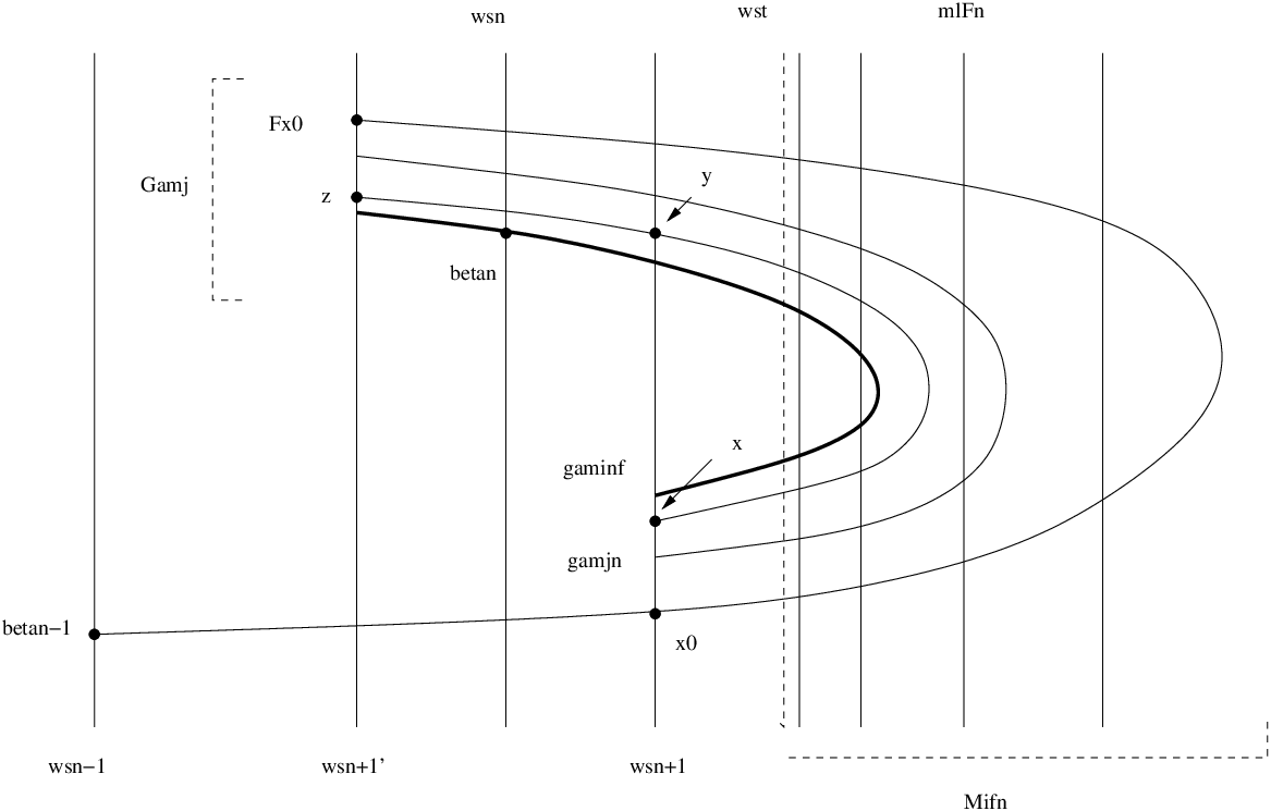
The proof of this Theorem needs some preparation. Let n≥1n\geq 1 and q1,q2,q3∈Wu​(βn−1)q_{1},q_{2},q_{3}\in W^{u}(\beta_{n-1}) be the first three intersections, coming from βn−1\beta_{n-1} along Wu​(βn−1)W^{u}(\beta_{n-1}), with Wlocs​(βn+1)W^{s}_{{\mathrm{loc}}}(\beta_{n+1}), and let q2′,q3′∈Wu​(βn−1)q^{\prime}_{2},q^{\prime}_{3}\in W^{u}(\beta_{n-1}) be the second and third intersection with Wlocs​(βn+1′)W^{s}_{{\mathrm{loc}}}(\beta^{\prime}_{n+1}). Now define the saddle-region TnT_{n} of βn\beta_{n} the domain containing βn\beta_{n} which is bounded by the following four arcs, [q2,q2′]u⊂Wu​(βn−1)[q_{2},q^{\prime}_{2}]^{u}\subset W^{u}(\beta_{n-1}), [q3,q3′]u⊂Wu​(βn−1)[q_{3},q^{\prime}_{3}]^{u}\subset W^{u}(\beta_{n-1}), [q2,q3]s⊂Ws​(βn+1)[q_{2},q_{3}]^{s}\subset W^{s}(\beta_{n+1}) and [q2′,q3′]s⊂Ws​(βn+1′)[q^{\prime}_{2},q^{\prime}_{3}]^{s}\subset W^{s}(\beta^{\prime}_{n+1}), see Figure  4.1.

Refer to caption
Figure 4.1. Saddle-region of βn\beta_{n}

Furthermore, let p0,p1∈Wu​(βn−1)p_{0},p_{1}\in W^{u}(\beta_{n-1}) be the first two intersections with Wlocs​(βn)W^{s}_{{\mathrm{loc}}}(\beta_{n}). The curve [p0,p1]u⊂Wu​(βn−1)[p_{0},p_{1}]^{u}\subset W^{u}(\beta_{n-1}) is a fundamental domain for FF restricted to Wu​(βn−1)W^{u}(\beta_{n-1}). Consider the following fundamental domain

Kn−1u=F−2n​([p0,p1]u).K^{u}_{n-1}=F^{-2^{n}}([p_{0},p_{1}]^{u}).

The connected components of Wu​(βn)∩TnW^{u}(\beta_{n})\cap T_{n} and Ws​(βn)∩TnW^{s}(\beta_{n})\cap T_{n} ( which contain βn\beta_{n}) are denoted by Un,Sn⊂TnU_{n},S_{n}\subset T_{n}. Notice, Sn∩Trapn+1=∅S_{n}\cap\operatorname{Trap}_{n+1}=\emptyset.

Lemma 4.7.

Wu​(βn)W^{u}(\beta_{n}) and Ws​(βn)W^{s}(\beta_{n}) are (non-compact) one-dimensional embedded manifolds, for each n≥0n\geq 0.

Proof.

For each n≥1n\geq 1 we have that the fundamental domain of Wu​(βn−1)W^{u}(\beta_{n-1}) satisfies F2n​(Kn−1u)⊂TrapnF^{2^{n}}(K^{u}_{n-1})\subset\operatorname{Trap}_{n}. Because Kn−1u∩Trapn=∅K^{u}_{n-1}\cap\operatorname{Trap}_{n}=\emptyset we have

⋃i≠0Fi​(Kn−1u)∖Kn−1u¯∩int⁡Kn−1u=∅.\overline{\bigcup_{i\neq 0}F^{i}(K^{u}_{n-1})\setminus K^{u}_{n-1}}\cap\operatorname{int}K^{u}_{n-1}=\emptyset.

This implies that Wu​(βn−1)W^{u}(\beta_{n-1}) does not accumulate at itself, it is a one-dimensional manifold.

The proof for the stable manifold is similar, we have to show that Ws​(βn)W^{s}(\beta_{n}) does not accumulate at itself. Suppose it does. Then for some s∈int⁡Sns\in\operatorname{int}S_{n} there exists a sequence Ws​(βn)∖Sn∋sk→sW^{s}(\beta_{n})\setminus S_{n}\ni s_{k}\to s. We may assume that each sk∈Tns_{k}\in T_{n}. Apply Lemma 4.2 to Rn​FR^{n}F and we get

βn∈ω⁡(sk)⊂Trapn+1.\beta_{n}\in\omega(s_{k})\subset\operatorname{Trap}_{n+1}.

Contradiction. ∎

Remark 4.3.

The unstable manifolds are connected. However, the stable manifold of a periodic points consists of countably many closed curves.

Lemma 4.8.

Let F∈ℋΩn​(ε¯)F\in{\mathcal{H}}^{n}_{\Omega}(\overline{{\varepsilon}}), with ε¯>0\overline{{\varepsilon}}>0 small enough. Then

Ws​(βn)∩Tn=Sn.W^{s}(\beta_{n})\cap T_{n}=S_{n}.
Proof.

Let Z3⊂BZ_{3}\subset B be the open domain bounded by M−1nM^{n}_{-1} and Wlocs​(βn)W^{s}_{\mathrm{loc}}(\beta_{n}) and Z4⊂BZ_{4}\subset B be the open domain bounded by M1nM^{n}_{1} and Wlocs​(βn)W^{s}_{\mathrm{loc}}(\beta_{n}), see Figure 3.1. Recall,

F2n​(Z3)⊂Z4F^{2^{n}}(Z_{3})\subset Z_{4}

and

F2n​(Z4)⊂Z3.F^{2^{n}}(Z_{4})\subset Z_{3}.

Hence, no point in Z3∪Z4Z_{3}\cup Z_{4} will ever enter Wlocs​(βn)W^{s}_{\mathrm{loc}}(\beta_{n}). This means

Ws​(βn)∩(Z3∪Z4)=∅.W^{s}(\beta_{n})\cap(Z_{3}\cup Z_{4})=\emptyset.

Finally, observe that Tn⊂Z3∪Wlocs∪Z4T_{n}\subset Z_{3}\cup W^{s}_{\mathrm{loc}}\cup Z_{4}. The Lemma follows. ∎

Lemma 4.9.

Let F∈ℋΩn+1​(ε¯)F\in{\mathcal{H}}^{n+1}_{\Omega}(\overline{{\varepsilon}}), with ε¯>0\overline{{\varepsilon}}>0 small enough. Then

Wu​(βn)¯∖Wu​(βn)=Wu​(βn+1)¯∪Wu​(βn+1′)¯.\overline{W^{u}(\beta_{n})}\setminus W^{u}(\beta_{n})=\overline{W^{u}(\beta_{n+1})}\cup\overline{W^{u}(\beta^{\prime}_{n+1})}.
Proof.

Applying Theorem  4.1 to R​FRF, we obtain:

(4.2) 𝒜F∖Wu​(β0)\displaystyle{\mathcal{A}}_{F}\setminus W^{u}(\beta_{0}) ={(𝒜F∩D1)∪(𝒜F∩F⁡(D1))}∖Wu​(β0)\displaystyle=\{({\mathcal{A}}_{F}\cap D_{1})\cup({\mathcal{A}}_{F}\cap F(D_{1}))\}\setminus W^{u}(\beta_{0})
=(Wu​(β1)¯∩D1)∪F⁡(Wu​(β1)¯∩D1)\displaystyle=(\overline{W^{u}(\beta_{1})}\cap D_{1})\cup F(\overline{W^{u}(\beta_{1})}\cap D_{1})
=Wu​(β1)¯.\displaystyle=\overline{W^{u}(\beta_{1})}.

Figure  4.1 might be useful in the following argument. Apply Theorem  4.1 and equation  (4.2) to Rn​FR^{n}F and we obtain

(Wu​(βn)¯∖Wu​(βn))∩Dn=Wu​(βn+1)¯.(\overline{W^{u}(\beta_{n})}\setminus W^{u}(\beta_{n}))\cap D_{n}=\overline{W^{u}(\beta_{n+1})}.

Observe that

Wu​(βn)¯⊂Dn∪F2n−1​(Dn).\overline{W^{u}(\beta_{n})}\subset D_{n}\cup F^{2^{n-1}}(D_{n}).

Hence,

Wu​(βn)¯∖Wu​(βn)=\displaystyle\overline{W^{u}(\beta_{n})}\setminus W^{u}(\beta_{n})=
((Wu​(βn)¯∖Wu​(βn))∩Dn)∪((Wu​(βn)¯∖Wu​(βn))∩F2n−1​(Dn))=\displaystyle((\overline{W^{u}(\beta_{n})}\setminus W^{u}(\beta_{n}))\cap D_{n})\cup((\overline{W^{u}(\beta_{n})}\setminus W^{u}(\beta_{n}))\cap F^{2^{n-1}}(D_{n}))=
((Wu​(βn)¯∖Wu​(βn))∩Dn)∪F2n−1​((Wu​(βn)¯∖Wu​(βn)∩Dn)=CLOSE\displaystyle((\overline{W^{u}(\beta_{n})}\setminus W^{u}(\beta_{n}))\cap D_{n})\cup F^{2^{n-1}}((\overline{W^{u}(\beta_{n})}\setminus W^{u}(\beta_{n})\cap D_{n})=
Wu​(βn+1)¯∪Wu​(βn+1′)¯.\displaystyle\overline{W^{u}(\beta_{n+1})}\cup\overline{W^{u}(\beta^{\prime}_{n+1})}.

∎

Define, for k<nk<n,

Ek,n={x∈Kk| ∃t>0 ∀j<t Fj(x)∉Tn and Ft(x)∈Tn}.E_{k,n}=\{x\in K_{k}|\text{ }\exists t>0\text{ }\forall j<t\text{ }F^{j}(x)\notin T_{n}\text{ and }F^{t}(x)\in T_{n}\}.

The time t>0t>0 in the above definition is called the time of entry of x∈Ek,nx\in E_{k,n} into TnT_{n}.

Definition 4.2.

Let k<nk<n. We say that FF satisfies the transversality condition 𝒯k,n\mathcal{T}_{k,n} if the following holds. Let zj∈Ek,nz_{j}\in E_{k,n}, j≥0j\geq 0, be a sequence such that

Ftj​(zj)→s∈Sn,F^{t_{j}}(z_{j})\rightarrow s\in S_{n},

where tj>0t_{j}>0 is the time of entry of zjz_{j} into TnT_{n}, then

D​Ftj​(zj)​(Tzj​Wu​(βk))↛Ts​Ws​(βn).DF^{t_{j}}(z_{j})(T_{z_{j}}W^{u}(\beta_{k}))\nrightarrow T_{s}W^{s}(\beta_{n}).
Definition 4.3.

A (k,n)(k,n)-heteroclinic tangency, k<nk<n, for an nn-times renormalizable Hénon map is a tangency between Wu​(βk)W^{u}(\beta_{k}) and Ws​(βn)W^{s}(\beta_{n}). If there is such a tangency we write

Wu​(βk)​−⁣−∩Ws​(βn).W^{u}(\beta_{k})\kern 6.99997pt\makebox[0.0pt][c]{\raisebox{3.31528pt}{$--$}}\kern-6.00006pt\cap\>W^{s}(\beta_{n}).

Let 𝒦k,n​(ε¯)⊂ℋΩn​(ε¯)\mathcal{K}_{k,n}(\overline{{\varepsilon}})\subset{\mathcal{H}}^{n}_{\Omega}(\overline{{\varepsilon}}) consists of the nn-times renormalizable maps which have a (k,n)−(k,n)-heteroclinic tangency and

𝒰​𝒦k,n​(ε¯)=⋃k≤k′<n′≤n𝒦k′,n′​(ε¯).{\mathcal{U}}{\mathcal{K}}_{k,n}(\overline{{\varepsilon}})=\bigcup_{k\leq k^{\prime}<n^{\prime}\leq n}{\mathcal{K}}_{k^{\prime},n^{\prime}}(\overline{{\varepsilon}}).
Proposition 4.10.

Let F∈ℋΩn​(ε¯)F\in{\mathcal{H}}^{n}_{\Omega}(\overline{{\varepsilon}}), ε¯>0\overline{{\varepsilon}}>0 small enough. Let k<nk<n and suppose that FF satisfies

F∉𝒰​𝒦k,n​(ε¯).F\notin{\mathcal{U}}{\mathcal{K}}_{k,n}(\overline{{\varepsilon}}).

Then 𝒯k,n\mathcal{T}_{k,n} holds.

Proof.

Fix k<nk<n and a sequence zj∈Ek,nz_{j}\in E_{k,n}, j≥0j\geq 0, with zj→zz_{j}\rightarrow z and

Ftj​(zj)→s∈Sn,F^{t_{j}}(z_{j})\rightarrow s\in S_{n},

where tj>0t_{j}>0 in the time of entry of zjz_{j} into TnT_{n}.

If the tjt_{j}’s are bounded, say constant tj=tt_{j}=t, the absence of heteroclinic tangencies, F∉𝒦k,n​(ε¯)F\notin{\mathcal{K}}_{k,n}(\overline{{\varepsilon}}), implies that

D​Ft​(z)​(Tz​Wu​(βk))≠Ts​Sn.DF^{t}(z)(T_{z}W^{u}(\beta_{k}))\neq T_{s}S_{n}.

Hence,

D​Ftj​(zj)​(Tzj​Wu​(βk))↛Ts​Sn.DF^{t_{j}}(z_{j})(T_{z_{j}}W^{u}(\beta_{k}))\nrightarrow T_{s}S_{n}.

Secondly, we will consider the case when the times tjt_{j} of entry are unbounded.

Claim 4.11.

There exists k<m1≤nk<m_{1}\leq n such that z∈Ek,m1∩Ws​(𝜷m1).z\in E_{k,m_{1}}\cap W^{s}({\mbox{\boldmath$\beta$}}_{m_{1}}).

Proof.

Theorem  4.1 describes the limit behavior of the orbit of zz. Assume,

ω⁡(z)⊂𝒪⁡(F)∪⋃j>n𝜷j.\omega(z)\subset{\mathcal{O}}(F)\cup\bigcup_{j>n}{\mbox{\boldmath$\beta$}}_{j}.

Then for some t>0t>0 we have Fi​(z)∈int⁡(Trapn+1)F^{i}(z)\in\operatorname{int}(\operatorname{Trap}_{n+1}) whenever i≥ti\geq t. This means that the orbit of zjz_{j}, j>0j>0 large enough, will also enter this trapping region after tt steps. For j>0j>0 large enough, tj>tt_{j}>t. This contradicts

Ftj​(zj)→s∉Trapn+1.F^{t_{j}}(z_{j})\to s\notin\operatorname{Trap}_{n+1}.

∎

Refer to caption
Figure 4.2.

Denote the time of entry of zz into Sm1⊂Tm1S_{m_{1}}\subset T_{m_{1}} by r1>0r_{1}>0 and let Fr1​(z)=s1F^{r_{1}}(z)=s_{1}. We will call r1r_{1} the first transient time. For j>0j>0 large enough, zj∈Ek,m1z_{j}\in E_{k,m_{1}} with corresponding entry time tj1=r1t^{1}_{j}=r_{1}. Note that m1<nm_{1}<n. Otherwise, the sequence consisting of tj=tj1=r1t_{j}=t_{j}^{1}=r_{1} would be bounded. The absence of heteroclinic tangencies, F∉𝒦k,m1​(ε¯)F\notin{\mathcal{K}}_{k,m_{1}}(\overline{{\varepsilon}}), implies that

D​Fr1​(z)​(Tz​Wu​(βk))≠Ts1​Sm1.DF^{r_{1}}(z)(T_{z}W^{u}(\beta_{k}))\neq T_{s_{1}}S_{m_{1}}.

Hence,

(4.3) D​Ftj1​(zj)​(Tzj​Wu​(βk))↛Ts1​Sm1.DF^{t^{1}_{j}}(z_{j})(T_{z_{j}}W^{u}(\beta_{k}))\nrightarrow T_{s_{1}}S_{m_{1}}.

Let ej1>0e^{1}_{j}>0 be maximal such that when r1≤i≤ej1r_{1}\leq i\leq e_{j}^{1} we have

Fi​(zj)∈Tm1.F^{i}(z_{j})\in T_{m_{1}}.

The moment ej1e^{1}_{j} is called the time of exit of zjz_{j} from Tm1T_{m_{1}}. We may assume that Fej1​(zj)→u1∈Um1F^{e^{1}_{j}}(z_{j})\rightarrow u_{1}\in U_{m_{1}}. Then  (4.3) implies, use the λ\lambda-Lemma from [dMP],

(4.4) D​Fej1​(zj)​(Tzj​Wu​(βk))→Tu1​Um1.DF^{e^{1}_{j}}(z_{j})(T_{z_{j}}W^{u}(\beta_{k}))\rightarrow T_{u_{1}}U_{m_{1}}.

Now, we can repeat the proof of Claim  4.11 and obtain m1<m2≤nm_{1}<m_{2}\leq n and r2>0r_{2}>0, the second transient time, such that

Fr2​(u1)=s2∈Sm2.F^{r_{2}}(u_{1})=s_{2}\in S_{m_{2}}.

For j>0j>0 large enough we have zj∈Ek,m2z_{j}\in E_{k,m_{2}}. Denote the time of entry of zjz_{j} into Tm2T_{m_{2}} by tj2>0t^{2}_{j}>0 then tj2=ej1+r2t^{2}_{j}=e^{1}_{j}+r_{2}. The absence of heteroclinic tangencies, F∉𝒦m1,m2​(ε¯)F\notin{\mathcal{K}}_{m_{1},m_{2}}(\overline{{\varepsilon}}), implies that

D​Fr2​(u1)​(Tu1​Wu​(βm1))≠Ts2​Sm2.DF^{r_{2}}(u_{1})(T_{u_{1}}W^{u}(\beta_{m_{1}}))\neq T_{s_{2}}S_{m_{2}}.

Hence,  (4.4) implies

(4.5) D​Ftj2​(zj)​(Tzj​Wu​(βk))↛Ts2​Sm2.DF^{t^{2}_{j}}(z_{j})(T_{z_{j}}W^{u}(\beta_{k}))\nrightarrow T_{s_{2}}S_{m_{2}}.

Let ej2>0e^{2}_{j}>0 be maximal such that when tj2≤i≤ej2t^{2}_{j}\leq i\leq e_{j}^{2} we have

Fi​(zj)∈Tm2.F^{i}(z_{j})\in T_{m_{2}}.

We may assume that Fej2​(zj)→u2∈Um2F^{e^{2}_{j}}(z_{j})\rightarrow u_{2}\in U_{m_{2}}. Then

(4.6) D​Fej2​(zj)​(Tzj​Wu​(βk))→Tu2​Um2.DF^{e^{2}_{j}}(z_{j})(T_{z_{j}}W^{u}(\beta_{k}))\rightarrow T_{u_{2}}U_{m_{2}}.

If m2=nm_{2}=n, statement  (4.5) proves the transversality property. In the case when m2<nm_{2}<n we can repeat this construction, and we get a sequence m1<m2<m3<⋯<mgm_{1}<m_{2}<m_{3}<\dots<m_{g} together with points sl∈Smls_{l}\in S_{m_{l}}, ul∈Umlu_{l}\in U_{m_{l}} and times of entry and exit tjl>0t^{l}_{j}>0 and ejl>0e^{l}_{j}>0 for zj∈Ek,mlz_{j}\in E_{k,m_{l}} and the corresponding asymptotic expressions  (4.3) and  (4.4).

The sequence mlm_{l} is strictly increasing. Hence, mg=nm_{g}=n and tj=tjgt_{j}=t^{g}_{j} for some g≥1g\geq 1. Now, statement  (4.3) corresponding to TmgT_{m_{g}},

D​Ftj​(zj)​(Tzj​Wu​(βk))↛Ts​SnDF^{t_{j}}(z_{j})(T_{z_{j}}W^{u}(\beta_{k}))\nrightarrow T_{s}S_{n}

finishes the proof of the Proposition. ∎

Proposition 4.12.

Let F∈ℋΩn​(ε¯)F\in{\mathcal{H}}^{n}_{\Omega}(\overline{{\varepsilon}}), with ε¯>0\overline{{\varepsilon}}>0 small enough, and k<nk<n. Assume

(4.7) F∉𝒰​𝒦k+1,n​(ε¯).F\notin{\mathcal{U}}{\mathcal{K}}_{k+1,n}(\overline{{\varepsilon}}).

Then

⋃k≤j≤nWu​(𝜷j)\bigcup_{k\leq j\leq n}W^{u}({\mbox{\boldmath$\beta$}}_{j})

is laminar.

Proof.

Choose k≤j≤nk\leq j\leq n. To prove that every point in Wu​(βj)W^{u}(\beta_{j}) is laminar it suffices to prove that every point z∈Ujz\in U_{j} is laminar. According to Lemma 4.9 Wu​(βj)W^{u}(\beta_{j}) is not accumulated by Wu​(βm)W^{u}(\beta_{m}) with m>jm>j. From Lemma  4.7 we have that Wu​(βj)W^{u}(\beta_{j}) is a one-dimensional embedded manifold. Hence, the only non-trivial accumulation is from Wu​(βl)W^{u}(\beta_{l}) with k≤l<jk\leq l<j. Assume that z∈Ujz\in U_{j} is not a laminar point. Let k≤l<jk\leq l<j and zm∈El,jz_{m}\in E_{l,j} be a sequence with

Fem​(zm)→zF^{e_{m}}(z_{m})\to z

but D​Fem​(zm)​(Tzm​Wu​(βl))DF^{e_{m}}(z_{m})(T_{z_{m}}W^{u}(\beta_{l})) stays away from Tz​UjT_{z}U_{j}. Let tm<emt_{m}<e_{m} be such that

Ftm​(zm)→s∈Sj.F^{t_{m}}(z_{m})\to s\in S_{j}.

Proposition 4.10 states that 𝒯l,j\mathcal{T}_{l,j} holds. Hence, for a subsequence, D​Ftm​(zm)​(Tzm​Wu​(βl))DF^{t_{m}}(z_{m})(T_{z_{m}}W^{u}(\beta_{l})) stays away from Ts​SjT_{s}S_{j}. Then again the λ\lambda-Lemma implies that for this subsequence

D​Fem​(zm)​(Tzm​Wu​(βl))→Tz​Uj.DF^{e_{m}}(z_{m})(T_{z_{m}}W^{u}(\beta_{l}))\rightarrow T_{z}U_{j}.

Contradiction. ∎

Proof of Theorem  4.6. Suppose, x∈Wu​(βn)x\in W^{u}(\beta_{n}) is a non-laminar point of 𝒜F{\mathcal{A}}_{F}. According to Lemma 4.9 this implies that this point is actually a non-laminar point of

⋃j≤nWu​(𝜷j).\bigcup_{j\leq n}W^{u}({\mbox{\boldmath$\beta$}}_{j}).

This contradicts Proposition 4.12. ∎

5. Conjugations

The boundary ∂B\partial B of the domain of a Hénon-like map F:B→BF:B\to B does not have dynamical meaning. Even if we restrict the map to B0¯\overline{B_{0}}, only an arc of ∂B0\partial B_{0}, namely Wlocs​(β0)W^{s}_{\mathrm{loc}}(\beta_{0}), is dynamically meaningful. The fact that the boundary is rather arbitrary entails that the notion of topological equivalence defined by conjugations h:B→h⁡(B)=B~h:B\to h(B)=\tilde{B} is too restrictive. For this reason, below we slightly relax this notion.

A relative neighborhood U⊂B¯0U\subset\bar{B}_{0} is an open set in the intrinsic topology of B0B_{0}. A conjugation between two Hénon-like maps F,F~∈ℐΩ​(ε¯)F,\tilde{F}\in{\mathcal{I}}_{\Omega}(\overline{{\varepsilon}}) is a homeomorphism h:U→h⁡(U)=U~h:U\to h(U)=\tilde{U} such that

  1. (1)

    U⊃𝒜FU\supset{\mathcal{A}}_{F} and U~⊃𝒜F~\tilde{U}\supset{\mathcal{A}}_{\tilde{F}} are relative neighborhoods in the corresponding boxes;

  2. (2)

    UU and U~\tilde{U} are forward invariant under the corresponding dynamics;

  3. (3)

    h∘F=F~∘hh\circ F=\tilde{F}\circ h.

Theorem 5.1.

Let h:U→U~h:U\to\tilde{U} be a conjugation between two infinitely renormalizable Hénon-like maps F,F~∈ℐΩ​(ε¯)F,\tilde{F}\in{\mathcal{I}}_{\Omega}(\overline{{\varepsilon}}), with ε¯>0\overline{{\varepsilon}}>0 small enough. Then

h(○ℤ(τF))=○ℤ(τF~).h(\text{$\mathchar 525$}_{\mathbb{Z}}(\tau_{F}))=\text{$\mathchar 525$}_{\mathbb{Z}}(\tau_{\tilde{F}}).

The dynamics of F|𝒪FF|{\mathcal{O}}_{F}, the adding machine, is homogeneous, in the sense that the group of automorphisms acts transitively on 𝒪F{\mathcal{O}}_{F} (here an automorphism is a homeomorphism commuting with FF). The situation is different when this Cantor set is embedded as the attractor of a Hénon-like map and the automorphism has an extension to a conjugation. Then, as the above Theorem shows, any automorphism has to preserve the orbit of the tip. This easily implies that the automorphism group is reduced to the cyclic group ℤ\mathbb{Z} of the iterates of F|𝒪FF|{\mathcal{O}}_{F}.

The proof of Theorem 5.1 needs some preparation. A map F∈ℐΩ​(ε¯)F\in{\mathcal{I}}_{\Omega}(\overline{{\varepsilon}}) has exactly two fixed points: β0\beta_{0} and β1\beta_{1}. The first has positive eigenvalues and the second one is of flip type, it has negative eigenvalues. The topological difference between the fixed points imply that every conjugation between two maps satisfies

h⁡(βi)=β~i,h(\beta_{i})=\tilde{\beta}_{i},

for i=0,1i=0,1. If a Hénon-like map FF is renormalizable then there is only one heteroclinic orbit coming from β0\beta_{0} and going to β1\beta_{1}:

Wu​(β0)∩Ws​(β1)={pi1}i∈ℤ,W^{u}(\beta_{0})\cap W^{s}(\beta_{1})=\{p^{1}_{i}\}_{i\in\mathbb{Z}},

with F⁡(pi1)=pi+11F(p^{1}_{i})=p^{1}_{i+1}. (The topological definition of renormalizable Hénon-like maps is discussed in §3.4 of [CLM]). Observe,

p01∈Wu​(β0)⊂U=Dom⁡(h).p^{1}_{0}\in W^{u}(\beta_{0})\subset U=\operatorname{Dom}(h).

Hence, every conjugation will satisfy

(5.1) h⁡(p01)=p~m1,h(p^{1}_{0})=\tilde{p}^{1}_{m},

for some m∈ℤm\in\mathbb{Z}.

In §3 the domain D1D_{1} was introduced, the domain of the first pre-renormalization F2|D1F^{2}|D_{1}. This topological disc is bounded by two curves ∂s⊂Ws(β1)\partial^{s}\subset W^{s}(\beta_{1}) and ∂u⊂Wu(β0)\partial^{u}\subset W^{u}(\beta_{0}) whose endpoints are p01p^{1}_{0} and p11p^{1}_{1}. The forward images of D1D_{1}, ∂s\partial^{s}, and ∂u\partial^{u} are denoted respectively by D1l=Fl​(D1)D_{1}^{l}=F^{l}(D_{1}), δls=Fl(∂s)\delta^{s}_{l}=F^{l}(\partial^{s}), and δlu=Fl(∂u)\delta^{u}_{l}=F^{l}(\partial^{u}), l≥0l\geq 0. The map Fl:D1→D1lF^{l}:D_{1}\to D^{l}_{1} is a diffeomorphism.

For l≥0l\geq 0, the curve δls⊂Ws​(β1)\delta^{s}_{l}\subset W^{s}(\beta_{1}) connects pl1p^{1}_{l} with pl+11p^{1}_{l+1}. On the other hand, for l<0l<0, and ε¯>0\overline{{\varepsilon}}>0 small enough, there is no arc in Ws​(β1)W^{s}(\beta_{1}) which connects pl1p^{1}_{l} with pl+11p^{1}_{l+1}. The connected components of Ws​(β1)W^{s}(\beta_{1}) that contain the points pl1p^{1}_{l}, l<0l<0, are pairwise disjoint. This is observed in §3, see Figure 3.1, and will be useful in what follows.

Lemma 5.2.

Let h:U→U~h:U\to\tilde{U} be a conjugation between F,F~∈ℐΩ​(ε¯)F,\tilde{F}\in{\mathcal{I}}_{\Omega}(\overline{{\varepsilon}}), F~∘h=h∘F.\tilde{F}\circ h=h\circ F. There exists k,l≥0k,l\geq 0 and a conjugation

h′:V→V~,h^{\prime}:V\to\tilde{V},

given by

h′=F~−l∘h∘Fkh^{\prime}=\tilde{F}^{-l}\circ h\circ F^{k}

such that

  1. (1)

    D1⊂VD_{1}\subset V, D~1⊂V~\tilde{D}_{1}\subset\tilde{V}, and

    h′​(D1)=D~1,h^{\prime}(D_{1})=\tilde{D}_{1},
  2. (2)

    for every x∈Vx\in V

    h′(○(Fl(x)))=h(○(Fk(x))).h^{\prime}(\text{$\mathchar 525$}(F^{l}(x)))=h(\text{$\mathchar 525$}(F^{k}(x))).
Proof.

Lemma 4.2 gives a k≥1k\geq 1 such that Fk​(B0¯)⊂UF^{k}(\overline{B_{0}})\subset U. Define a conjugation

h1:B0→h1​(B0)⊂U~⊂B0,h_{1}:B_{0}\to h_{1}(B_{0})\subset\tilde{U}\subset B_{0},

by h1=h∘Fk.h_{1}=h\circ F^{k}. Observe that the maps hh and h1h_{1} act in the same way on the space of orbits. In particular, equation (5.1) gives some l∈ℤl\in\mathbb{Z} such that

h1​(p01)=p~l1.h_{1}(p^{1}_{0})=\tilde{p}^{1}_{l}.

The curve ∂s⊂Ws(β1)\partial^{s}\subset W^{s}(\beta_{1}) connects p01p^{1}_{0} with p11p^{1}_{1}. Hence, the points p~l1\tilde{p}^{1}_{l} and p~l+11\tilde{p}^{1}_{l+1} are connected by a curve in the stable manifold of β~1\tilde{\beta}_{1}. So, l≥0l\geq 0. The domain of h1h_{1}, Dom⁡(h1)=B\operatorname{Dom}(h_{1})=B, contains D1D_{1}. Actually, h1h_{1} matches the boundaries ∂u,s\partial^{u,s} of D1D_{1} with the boundaries δ~u,s\tilde{\delta}^{u,s} of D~1l\tilde{D}^{l}_{1}. Hence,

h1​(D1)=D~1l.h_{1}(D_{1})=\tilde{D}^{l}_{1}.

As was noticed previously, the map

F~−l:D~1l∩𝒜F~→D~1∩𝒜F~\tilde{F}^{-l}:\tilde{D}^{l}_{1}\cap{\mathcal{A}}_{\tilde{F}}\to\tilde{D}_{1}\cap{\mathcal{A}}_{\tilde{F}}

is a well-defined homeomorphism because l≥0l\geq 0. Choose a relatively open F~\tilde{F}-forward invariant set V~′⊂B0\tilde{V}^{\prime}\subset B_{0} satisfying

D~1l∪𝒜F~⊂V~′⊂h1​(B0),\tilde{D}^{l}_{1}\cup{\mathcal{A}}_{\tilde{F}}\subset\tilde{V}^{\prime}\subset h_{1}(B_{0}),

and small enough such that F~−l|V~′\tilde{F}^{-l}|\tilde{V}^{\prime} is a well-defined diffeomorphism. Let

V=h1−1​(V~′),V=h_{1}^{-1}(\tilde{V}^{\prime}),
V~=F~−l​(V~′),\tilde{V}=\tilde{F}^{-l}(\tilde{V}^{\prime}),

and let h′:V→V~h^{\prime}:V\to\tilde{V} be defined by

h′=F~−l∘h1=F~−l∘h∘Fk.h^{\prime}=\tilde{F}^{-l}\circ h_{1}=\tilde{F}^{-l}\circ h\circ F^{k}.

By construction this conjugation satisfies h′​(D1)=D~1.h^{\prime}(D_{1})=\tilde{D}_{1}. ∎

According to the previous Lemma, we can replace any conjugation by another one which matches the first pre-renormalization domains D1D_{1} and D~1\tilde{D}_{1}, and coincides with the original conjugation on the space of orbits. The following Proposition will complete the proof of Theorem 5.1.

Proposition 5.3.

Let h:U→U~h:U\to\tilde{U} be a conjugation between two infinitely renormalizable Hénon-like maps F,F~∈ℐΩ​(ε¯)F,\tilde{F}\in{\mathcal{I}}_{\Omega}(\overline{{\varepsilon}}), with ε¯>0\overline{{\varepsilon}}>0 small enough. If h⁡(D1)=D~1h(D_{1})=\tilde{D}_{1} then

h⁡(Dn)=D~n,h(D_{n})=\tilde{D}_{n},

for all n≥1n\geq 1. In particular, h⁡(τF)=τF~h(\tau_{F})=\tau_{\tilde{F}}.

Refer to caption
Figure 5.1. Domains of pre-renormalizations
Proof.

First notice that for all n≥0n\geq 0 we have Dn⊂D1⊂Dom⁡(h)D_{n}\subset D_{1}\subset\operatorname{Dom}(h) and D~n⊂D~1⊂Im⁡(h)\tilde{D}_{n}\subset\tilde{D}_{1}\subset\operatorname{Im}(h). So, h⁡(Dn)h(D_{n}) is well defined.

The proof will be by induction. Assume that h⁡(Dk)=D~kh(D_{k})=\tilde{D}_{k}, for k≤nk\leq n. There exists a unique periodic point of period 2k+12^{k+1} in DkD_{k}. Namely, βk+1∈int⁡(Dk)\beta_{k+1}\in\operatorname{int}(D_{k}), k≤nk\leq n. In particular, h⁡(βk)=β~kh(\beta_{k})=\tilde{\beta}_{k}, with k≤n+1k\leq n+1.

Proposition 3.5 gives that both components of Wlocs​(βn+1)∖{βn+1}W^{s}_{{\mathrm{loc}}}(\beta_{n+1})\setminus\{\beta_{n+1}\} intersect ∂nu\partial^{u}_{n}. Let x0,x1∈Wlocs(βn+1)∩∂nux_{0},x_{1}\in W^{s}_{{\mathrm{loc}}}(\beta_{n+1})\cap\partial^{u}_{n} be the boundary points of the connected component of Ws​(βn+1)∩DnW^{s}(\beta_{n+1})\cap D_{n} containing βn+1\beta_{n+1}. Say x0x_{0} is the first and x1x_{1} is the second intersection of Wu​(βn−1)W^{u}(\beta_{n-1}) with the connected component of Ws​(βn+1)∩DnW^{s}(\beta_{n+1})\cap D_{n} which contains βn+1\beta_{n+1}. These points are topologically defined. As was noticed before, h⁡(βk)=β~kh(\beta_{k})=\tilde{\beta}_{k}, with k=n−1,n+1k=n-1,n+1. Hence, for i=0,1i=0,1,

h⁡(xi)=x~i.h(x_{i})=\tilde{x}_{i}.

Let γ⊂Wlocs​(βn+1)\gamma\subset W^{s}_{{\mathrm{loc}}}(\beta_{n+1}) bounded by x0x_{0} and x1x_{1}. Then

h⁡(γ)=γ~.h(\gamma)=\tilde{\gamma}.

Define En⊂DnE_{n}\subset D_{n} to be the connected component of Dn∖γD_{n}\setminus\gamma which does not contain βn\beta_{n}. Then

h⁡(En)=E~n.h(E_{n})=\tilde{E}_{n}.

Observe,

Dn+1⊂En.D_{n+1}\subset E_{n}.

Let y0,y1∈Wu​(βn)∩γy_{0},y_{1}\in W^{u}(\beta_{n})\cap\gamma be the first and second intersections of Wu​(βn)W^{u}(\beta_{n}) and γ\gamma. Then for i=0,1i=0,1

h⁡(yi)=y~i.h(y_{i})=\tilde{y}_{i}.

Notice, that the arc between y0y_{0} and y1y_{1} in Wu​(βn)W^{u}(\beta_{n}) equals ∂n+1u\partial^{u}_{n+1}. Furthermore, the arc between y0y_{0} and y1y_{1} in Ws​(βn+1)W^{s}(\beta_{n+1}) equals ∂n+1s\partial^{s}_{n+1}. Hence, the boundary of Dn+1D_{n+1} is matched to the boundary of D~n+1\tilde{D}_{n+1}. This finishes the induction step, h⁡(Dn+1)=D~n+1.h(D_{n+1})=\tilde{D}_{n+1}. ∎

Remark 5.1.

Without loss of generality we will only consider conjugations which match the tips of the maps under consideration.

6. Heteroclinic tangencies

If there is a heteroclinic tangency between Wu​(βk)W^{u}(\beta_{k}) and Ws​(βn)W^{s}(\beta_{n}) then βn∈𝒜F\beta_{n}\in{\mathcal{A}}_{F} is not a laminar point. Under this circumstances there will be non-periodic points which are non-laminar. Let 𝒞F⊂𝒜F{\mathcal{C}}_{F}\subset{\mathcal{A}}_{F} consists of the non-laminar points. Note, 𝒪F⊂𝒞F{\mathcal{O}}_{F}\subset{\mathcal{C}}_{F}.

Any map F∈ℋΩn​(ε¯)F\in{\mathcal{H}}^{n}_{\Omega}(\overline{{\varepsilon}}), with ε¯>0\overline{{\varepsilon}}>0 small enough, has a unique periodic orbit of period 2k−12^{k-1}, it is the orbit of βk\beta_{k}. Let λk∈(−1,0]\lambda_{k}\in(-1,0] and μk<−1\mu_{k}<-1 be the stable and unstable multiplier. The attractor at the nt​hn^{th}-scale is

𝒜Fn=○(Ψ0n(𝒜Rn​F))⊂𝒜F,n≥0.{\mathcal{A}}_{F}^{n}=\text{$\mathchar 525$}(\Psi_{0}^{n}({\mathcal{A}}_{R^{n}F}))\subset{\mathcal{A}}_{F},\quad n\geq 0.
Theorem 6.1.

If the infinitely renormalizable Hénon map F∈ℐΩ​(ε¯)F\in{\mathcal{I}}_{\Omega}(\overline{{\varepsilon}}), with ε¯>0\overline{{\varepsilon}}>0 small enough, has an (k,n)(k,n)-heteroclinic tangency and

ln⁡|λk|ln⁡|μn|∉ℚ\frac{\ln|\lambda_{k}|}{\ln|\mu_{n}|}\notin\mathbb{Q}

then

𝒜Fn⊂𝒞F.{\mathcal{A}}_{F}^{n}\subset\mathcal{C}_{F}.
Proof.

We can choose a C1C^{1}-coordinate system for TnT_{n} such that UnU_{n} and SnS_{n} are part of the xx-axis and yy-axis resp and that F2nF^{2^{n}} becomes linear with exponents λn\lambda_{n} and μn\mu_{n}, see [H]. Consider the fundamental domain [1,μn2]u⊂Un[1,\mu_{n}^{2}]^{u}\subset U_{n}. Let z∈Snz\in S_{n} be a (k,n)(k,n)-heteroclinic tangency.

Observe, that there are components of Wj⊂Wu​(βk−1)∩TkW_{j}\subset W^{u}(\beta_{k-1})\cap T_{k}, j≥1j\geq 1, which accumulate from both sides and in C3C^{3} sense on UkU_{k} and they are dynamically related. Namely,

F−2k​(Wj+1)⊂Wj.F^{-2^{k}}(W_{j+1})\subset W_{j}.

This laminar structure of Wu​(βk−1)W^{u}(\beta_{k-1}) around UkU_{k} will also be visible in a neighborhood of z∈Snz\in S_{n}. Because of the tangency at z∈Snz\in S_{n} there will be a sequence of points ej∈Wu​(βk−1)e_{j}\in W^{u}(\beta_{k-1}) with vertical tangent accumulating at z∈Snz\in S_{n}.

Refer to caption
Figure 6.1.

Let xjx_{j} be the xx-coordinate of eje_{j}. Then there is some ρ<1\rho<1 and C>0C>0 such that

xj=C⋅(1+O⁡(ρj))⋅λkj.x_{j}=C\cdot(1+O(\rho^{j}))\cdot\lambda_{k}^{j}.

Notice that accumulation points of Orb​({ej|j>0})\text{Orb}(\{e_{j}|j>0\}) on UnU_{n} are non-laminar points.

For j>0j>0 even, let sj>0s_{j}>0 be the (even) moment when Fsj​(ej)F^{s_{j}}(e_{j}) is above [1,μn2]u[1,\mu_{n}^{2}]^{u},

xj⋅μnsj∈[1,μn2]u.x_{j}\cdot\mu_{n}^{s_{j}}\in[1,\mu_{n}^{2}]^{u}.

Let A=ln⁡C/ln⁡μnA=\ln C/\ln\mu_{n} then

sj+j​ln⁡|λk|ln⁡|μn|+O⁡(ρj)+A=hj∈[0,2].s_{j}+j\frac{\ln|\lambda_{k}|}{\ln|\mu_{n}|}+O(\rho^{j})+A=h_{j}\in[0,2].

Hence,

hj2=sj2+12⋅(j⋅ln⁡|λk|ln⁡|μn|+A)+O⁡(ρj)∈[0,1].\frac{h_{j}}{2}=\frac{s_{j}}{2}+\frac{1}{2}\cdot(j\cdot\frac{\ln|\lambda_{k}|}{\ln|\mu_{n}|}+A)+O(\rho^{j})\in[0,1].

Because sjs_{j} is even we have

hj=2​{12⋅j⋅ln⁡|λk|ln⁡|μn|+A}+O⁡(ρj),h_{j}=2\{\frac{1}{2}\cdot j\cdot\frac{\ln|\lambda_{k}|}{\ln|\mu_{n}|}+A\}+O(\rho^{j}),

where {.}\{.\} stand for the fractional part. The sequence hjh_{j} is dense in [0,2][0,2] because ln⁡|λk|ln⁡|μn|\frac{\ln|\lambda_{k}|}{\ln|\mu_{n}|} is irrational. Now, let x^j\hat{x}_{j} be the projection of Fsj​(ej)F^{s_{j}}(e_{j}) on UnU_{n}. Then

x^j=μnhj.\hat{x}_{j}=\mu_{n}^{h_{j}}.

We proved that 𝒞F\mathcal{C}_{F} contains a fundamental domain of Wu​(βn)W^{u}(\beta_{n}). Namely,

[1,μn2]u⊂𝒞F.[1,\mu_{n}^{2}]^{u}\subset\mathcal{C}_{F}.

The set 𝒞F\mathcal{C}_{F} is closed and invariant. Apply Theorem  4.1 and the proof is finished. ∎

Corollary 6.2.

For ε¯>0\overline{{\varepsilon}}>0 small enough, for every k<nk<n there exists a dense GδG_{\delta} of infinitely renormalizable maps F∈𝒦k,n​(ε¯)∩ℐΩ​(ε¯)F\in\mathcal{K}_{k,n}(\overline{{\varepsilon}})\cap{\mathcal{I}}_{\Omega}(\overline{{\varepsilon}}) such that

𝒜Fn⊂𝒞F.{\mathcal{A}}_{F}^{n}\subset\mathcal{C}_{F}.

7. Location of the tip

In this section we will give quantitative information on the location of the tip. Let F∈ℐΩ​(ϵ¯)F\in{\mathcal{I}}_{\Omega}(\overline{\epsilon}), ϵ¯>0\overline{\epsilon}>0 small enough. The domain bounded by Wlocs​(β2)W^{s}_{\mathrm{loc}}(\beta_{2}) and Wlocs​(β2′)W^{s}_{\mathrm{loc}}(\beta^{\prime}_{2}) is called the extended saddle region and denoted by X⊂BX\subset B.

Consider the following family 𝒲\mathcal{W} of curves. A curve γ⊂X\gamma\subset X is in 𝒲\mathcal{W} if it is the graph of a C2C^{2}-function, also denoted by γ\gamma, with

γ:[xγ′,xγ]→ℝ,\gamma:[x^{\prime}_{\gamma},x_{\gamma}]\rightarrow\mathbb{R},

such that

(xγ′,γ⁡(xγ′))∈Wlocs​(β2′)(x^{\prime}_{\gamma},\gamma(x^{\prime}_{\gamma}))\in W^{s}_{\mathrm{loc}}(\beta^{\prime}_{2})

and

(xγ,γ⁡(xγ))∈Wlocs​(β2).(x_{\gamma},\gamma(x_{\gamma}))\in W^{s}_{\mathrm{loc}}(\beta_{2}).

We will use the notation γ∞=U1∈𝒲\gamma_{\infty}=U_{1}\in\mathcal{W}, (see Figure 4.1 to recall the definition of U1⊂BU_{1}\subset B). The distance dist⁡(γ,γ∞)\operatorname{dist}(\gamma,\gamma_{\infty}) is the C2C^{2}-norm between the corresponding functions measured on the domain of γ\gamma. Note that we can always extend γ∞\gamma_{\infty} within Wlocu​(β1)W^{u}_{\mathrm{loc}}(\beta_{1}) such that the corresponding domain of this extended function contains the domain [xγ′,xγ][x^{\prime}_{\gamma},x_{\gamma}] of any function γ∈𝒲\gamma\in\mathcal{W}.

Let Γ=F⁡(γ)\Gamma=F(\gamma), with γ∈𝒲\gamma\in\mathcal{W}. In particular, Γ∞=F⁡(γ∞)⊃γ∞\Gamma_{\infty}=F(\gamma_{\infty})\supset\gamma_{\infty}. Note that each curve Γ\Gamma can be described as a graph over the yy-axis,

Γ:[yγ′,yγ]→ℝ.\Gamma:[y^{\prime}_{\gamma},y_{\gamma}]\rightarrow\mathbb{R}.

This is a consequence of the fact that Hénon-like maps map vertical lines to horizontal lines, y′=xy^{\prime}=x. Moreover,

(Γ⁡(yγ),yγ)∈Wlocs​(β2′)(\Gamma(y_{\gamma}),y_{\gamma})\in W^{s}_{\mathrm{loc}}(\beta^{\prime}_{2})

and

(Γ⁡(yγ′),yγ′)∈Wlocs​(β2).(\Gamma(y^{\prime}_{\gamma}),y^{\prime}_{\gamma})\in W^{s}_{\mathrm{loc}}(\beta_{2}).

Indeed, we will consider the curves Γ=F⁡(γ)\Gamma=F(\gamma) as graphs over the y−y-axis. Note that we can always extend Γ∞\Gamma_{\infty} within Wlocu​(β1)W^{u}_{\mathrm{loc}}(\beta_{1}) such that the corresponding domain of the extension contains the domain [yγ′,yγ][y^{\prime}_{\gamma},y_{\gamma}] of any function Γ\Gamma. The distance dist⁡(Γ,Γ∞)\operatorname{dist}(\Gamma,\Gamma_{\infty}) is the C2C^{2}-norm between the corresponding functions measured on the domain of Γ\Gamma.

The map FF acts on 𝒲\mathcal{W} as a graph transform. Namely, the curve Wlocs​(β2)W^{s}_{\mathrm{loc}}(\beta_{2}) divide each Γ\Gamma into two components. One of which, denoted by 𝒯F​(γ){\mathcal{T}}_{F}(\gamma), is in 𝒲\mathcal{W},

𝒯F:γ↦F⁡(γ)∩X.{\mathcal{T}}_{F}:\gamma\mapsto F(\gamma)\cap X.
Refer to caption
Figure 7.1.
Proposition 7.1.

There exists C>0C>0, such that for all F∈ℐΩ​(ϵ¯)F\in{\mathcal{I}}_{\Omega}(\overline{\epsilon}), ϵ¯>0\overline{\epsilon}>0 small enough, the following holds:

(7.1) dist⁡(Γ,Γ∞)≤C⋅bF⋅dist⁡(γ,γ∞)\operatorname{dist}(\Gamma,\Gamma_{\infty})\leq C\cdot b_{F}\cdot\operatorname{dist}(\gamma,\gamma_{\infty})

and

(7.2) dist⁡(𝒯F​(γ),γ∞)≤C⋅bF⋅dist⁡(γ,γ∞).\operatorname{dist}({\mathcal{T}}_{F}(\gamma),\gamma_{\infty})\leq C\cdot b_{F}\cdot\operatorname{dist}(\gamma,\gamma_{\infty}).

If |γ⁡(x)−γ∞​(x)|∈[δ1,δ2]|\gamma(x)-\gamma_{\infty}(x)|\in[\delta_{1},\delta_{2}] with x∈[xγ′,xγ]x\in[x^{\prime}_{\gamma},x_{\gamma}] then

(7.3) |𝒯F​(γ)​(x)−γ∞​(x)|∈[1C⋅bF⋅δ1,C⋅bF⋅δ2],|{\mathcal{T}}_{F}(\gamma)(x)-\gamma_{\infty}(x)|\in[\frac{1}{C}\cdot b_{F}\cdot\delta_{1},C\cdot b_{F}\cdot\delta_{2}],

for x∈[x𝒯F​(γ)′,x𝒯F​(γ)]x\in[x^{\prime}_{{\mathcal{T}}_{F}(\gamma)},x_{{\mathcal{T}}_{F}(\gamma)}] and

(7.4) |Γ⁡(y)−Γ∞​(y)|∈[1C⋅bF⋅δ1,C⋅bF⋅δ2],|\Gamma(y)-\Gamma_{\infty}(y)|\in[\frac{1}{C}\cdot b_{F}\cdot\delta_{1},C\cdot b_{F}\cdot\delta_{2}],

for y∈[yγ′,yγ]y\in[y^{\prime}_{\gamma},y_{\gamma}].

Proof.

Let F∈ℐΩ​(ϵ¯)F\in{\mathcal{I}}_{\Omega}(\overline{\epsilon}), say F⁡(x,y)=(f⁡(x)−ϵ⁡(x,y),x)F(x,y)=(f(x)-\epsilon(x,y),x). Inspired by Theorem 7.9 from [CLM], we use the following representation

ϵ⁡(x,y)=bF​a​(x)​y​(1+m⁡(x,y)).\epsilon(x,y)=b_{F}a(x)y(1+m(x,y)).

The correction term mm is uniformly bounded for F∈ℐΩ​(ϵ¯)F\in{\mathcal{I}}_{\Omega}(\overline{\epsilon}). The specific form of a Hénon-like map, F⁡(x,y)=(f⁡(x)−ϵ⁡(x,y),x)F(x,y)=(f(x)-\epsilon(x,y),x), implies

Γ⁡(y)−Γ∞​(y)=\displaystyle\Gamma(y)-\Gamma_{\infty}(y)= −ϵ⁡(y,γ⁡(y))−ϵ⁡(y,γ∞​(y))\displaystyle-\epsilon(y,\gamma(y))-\epsilon(y,\gamma_{\infty}(y))
=\displaystyle= −bFa(y)⋅(γ(y)−γ∞(y))+\displaystyle-b_{F}a(y)\cdot(\gamma(y)-\gamma_{\infty}(y))+
−bFa(y)⋅(γ(y)−γ∞(y))⋅m(y,γ(y))+\displaystyle-b_{F}a(y)\cdot(\gamma(y)-\gamma_{\infty}(y))\cdot m(y,\gamma(y))+
−bFa(y)⋅γ∞(y)⋅(m(y,γ(y))−m(y,γ∞(y)).\displaystyle-b_{F}a(y)\cdot\gamma_{\infty}(y)\cdot(m(y,\gamma(y))-m(y,\gamma_{\infty}(y)).

The uniform bounds on mm and its derivatives give immediately the Properties (7.1) and (7.4).

Let γ0:x↦0\gamma_{0}:x\mapsto 0. The expression F⁡(x,y)=(f⁡(x)−ϵ⁡(x,y),x)F(x,y)=(f(x)-\epsilon(x,y),x) implies that Γ0\Gamma_{0} is the graph of the unimodal map ff. Let Y⊂Dom⁡(Γ0)Y\subset\operatorname{Dom}(\Gamma_{0}) be such that the graph of Γ0|Y⊂X\Gamma_{0}|Y\subset X, the extended saddle region. The graph of ff has its maximum outside the extended saddle region. This implies that

|D​Γ0|​Y|≥δ>0.|D\Gamma_{0}|Y|\geq\delta>0.

Also

|D​Γ∞|​Y|≥12​δ>0,|D\Gamma_{\infty}|Y|\geq\frac{1}{2}\delta>0,

which holds because of (7.1):

dist⁡(Γ0,Γ∞)=O⁡(bF).\operatorname{dist}(\Gamma_{0},\Gamma_{\infty})=O(b_{F}).

Now, use in the above expression for the difference of Γ⁡(y)\Gamma(y) and Γ∞​(y)\Gamma_{\infty}(y) the fact that the derivative of Γ∞|Y\Gamma_{\infty}|Y is away from zero: Properties (7.2) and (7.3) follow. ∎

Remark 7.1.

According to Theorem 7.9 from [CLM] the correction term mnm_{n} of Rn​FR^{n}F decays exponentially.

Let q1′,q1∈Wu​(β0)q^{\prime}_{1},q_{1}\in W^{u}(\beta_{0}) be the the first intersection, coming from β0\beta_{0} along Wu​(β0)W^{u}(\beta_{0}), with Wlocs​(β2′)W^{s}_{\mathrm{loc}}(\beta^{\prime}_{2}) and Wlocs​(β2)W^{s}_{\mathrm{loc}}(\beta_{2}), compare Figure 4.1. Consider the corresponding curve γ1=[q1′,q1]u⊂Wu​(β0)\gamma_{1}=[q^{\prime}_{1},q_{1}]^{u}\subset W^{u}(\beta_{0}). Note, γ1∈𝒲\gamma_{1}\in\mathcal{W}. Let

γi=𝒯Fi−1(γ1), i=2,3,…\gamma_{i}={\mathcal{T}}_{F}^{i-1}(\gamma_{1}),\text{ }i=2,3,\dots

The curves

Γi=F(γi−1)⊃γi, i=2,3,…\Gamma_{i}=F(\gamma_{i-1})\supset\gamma_{i},\text{ }i=2,3,\dots

will be used to locate the tip.

Corollary 7.2.

There exists C>0C>0, independent of the particular F∈ℐΩ​(ϵ¯)F\in{\mathcal{I}}_{\Omega}(\overline{\epsilon}), such that for i≥2i\geq 2

dist⁡(Γi,Γ∞)≤Ci⋅bFi−1\operatorname{dist}(\Gamma_{i},\Gamma_{\infty})\leq C^{i}\cdot b_{F}^{i-1}

and

1Ci⋅bFi−1≤|Γi​(y)−Γ∞​(y)|≤Ci⋅bFi−1,\frac{1}{C^{i}}\cdot b_{F}^{i-1}\leq|\Gamma_{i}(y)-\Gamma_{\infty}(y)|\leq C^{i}\cdot b_{F}^{i-1},

for y∈Dom⁡(Γi)y\in\operatorname{Dom}(\Gamma_{i}).

Lemma 7.3.

There exist unique points vi∈Γiv_{i}\in\Gamma_{i}, i≥2i\geq 2, and v∞∈Γ∞v_{\infty}\in\Gamma_{\infty} with a vertical tangent direction. Moreover,

d​Γid​y≍−(y−vi), i=2,3,…,∞.\frac{d\Gamma_{i}}{dy}\asymp-(y-v_{i}),\text{ }i=2,3,\dots,\infty.
Proof.

Let F⁡(x,y)=(f⁡(x)−ϵ⁡(x,y),x)F(x,y)=(f(x)-\epsilon(x,y),x) and γ0:x↦0\gamma_{0}:x\mapsto 0. Then Γ0=F⁡(γ0)\Gamma_{0}=F(\gamma_{0}) is the graph of ff over the y−y-axis. Proposition  7.1 and Corollary  7.2 imply that in C2C^{2} sense we have

dist⁡(Γ0,Γi)≤dist⁡(Γ0,Γ∞)+dist⁡(Γ∞,Γi)≤C⋅bF+Ci⋅bFi−1<<1,\operatorname{dist}(\Gamma_{0},\Gamma_{i})\leq\operatorname{dist}(\Gamma_{0},\Gamma_{\infty})+\operatorname{dist}(\Gamma_{\infty},\Gamma_{i})\leq C\cdot b_{F}+C^{i}\cdot b^{i-1}_{F}<<1,

for i=2,3​…i=2,3\dots. The Lemma follows because ff has a non degenerate critical point. ∎

Let aa be the intersection point of the horizontal line through τ=τF\tau=\tau_{F} and Γ2\Gamma_{2}. Note, aa is to the right of τ\tau. In case we are analyzing these points of the renormalization Rk​FR^{k}F, we will use the notation vik∈Γikv^{k}_{i}\in\Gamma^{k}_{i}, i=2,3,…,∞i=2,3,\dots,\infty, the points with vertical tangency.

Proposition 7.4.

For all F∈ℐΩ​(ϵ¯)F\in{\mathcal{I}}_{\Omega}(\overline{\epsilon}), ϵ¯>0\overline{\epsilon}>0 small enough, the following holds.

  1. (1)

    |π1​(v2)−π1​(a)|=O⁡(bF2)|\pi_{1}(v_{2})-\pi_{1}(a)|=O(b_{F}^{2}),

  2. (2)

    |π2​(v2)−π2​(a)|=O⁡(bF)|\pi_{2}(v_{2})-\pi_{2}(a)|=O(b_{F}),

  3. (3)

    |v2−τ|=O⁡(bF)|v_{2}-\tau|=O(b_{F}),

  4. (4)

    |τ−a|≍bF|\tau-a|\asymp b_{F}.

Remark 7.2.

The proof of Proposition 7.4 is illustrated with Figures 7.2 and 7.3. The xx-direction has been stretched dramatically.The analysis is done in a small neighborhood of v∞k+1v^{k+1}_{\infty} in Figure 7.2 and around v∞v_{\infty} in Figure 7.3. So, in the actual picture the curves are essentially straight vertical lines and the difference between the xx-coordinates x^k+1\hat{x}_{k+1}, xk+1x_{k+1}, and xk+1′x^{\prime}_{k+1} would be invisible.

Refer to caption
Figure 7.2.
Proof.

Take k≥0k\geq 0 and consider Rk+1​FR^{k+1}F. Observe,

v∞k∈Φkk+1​(Γ2k+1)⊂Φkk+1​(Wu​(β0​(Rk+1​F))).v^{k}_{\infty}\in\Phi^{k+1}_{k}(\Gamma^{k+1}_{2})\subset\Phi^{k+1}_{k}(W^{u}(\beta_{0}(R^{k+1}F))).

So, we can choose a point v^∞k+1∈Γ2k+1⊂Ωk+1\hat{v}^{k+1}_{\infty}\in\Gamma^{k+1}_{2}\subset\Omega_{k+1} such that

Φkk+1​(v^∞k+1)=v∞k∈D2​(Rk​F).\Phi^{k+1}_{k}(\hat{v}^{k+1}_{\infty})=v^{k}_{\infty}\in D_{2}(R^{k}F).

In coordinates, see Figure 7.2,

v^∞k+1=(x^k+1,y^k+1)\hat{v}^{k+1}_{\infty}=(\hat{x}_{k+1},\hat{y}_{k+1})

and

v∞k+1=(xk+1,yk+1).v^{k+1}_{\infty}=(x_{k+1},y_{k+1}).

Remember,

Λk∘Hk≡(Φkk+1)−1,\Lambda_{k}\circ H_{k}\equiv(\Phi^{k+1}_{k})^{-1},

with

Hk​(x,y)=(fk​(x)−ϵk​(x,y),y).H_{k}(x,y)=(f_{k}(x)-\epsilon_{k}(x,y),y).

The affine map Λk\Lambda_{k} is a dilatation. Consider D​HkDH_{k} and observe that this derivative maps the vertical tangent vector at v∞kv^{k}_{\infty} to Γ∞k\Gamma^{k}_{\infty} to an almost vertical vector. The angle between the image vector and the vertical is of the order bF2kb_{F}^{2^{k}}. Then, because v^∞k+1=Λk∘Hk​(v∞k)\hat{v}^{k+1}_{\infty}=\Lambda_{k}\circ H_{k}(v^{k}_{\infty}) and D​Γ∞k​(yk)=0D\Gamma^{k}_{\infty}(y_{k})=0, we get

(7.5) |D​Γ2k+1​(y^k+1)|=O⁡(bF2k).|D\Gamma^{k+1}_{2}(\hat{y}_{k+1})|=O(b_{F}^{2^{k}}).

Let

xk+1′=π1​(Γ2k+1​(yk+1)).x^{\prime}_{k+1}=\pi_{1}(\Gamma^{k+1}_{2}(y_{k+1})).

Corollary 7.2 gives

(7.6) |xk+1−xk+1′|≍bF2k+1|x_{k+1}-x^{\prime}_{k+1}|\asymp b_{F}^{2^{k+1}}

and

(7.7) |D​Γ2k+1​(yk+1)|=O⁡(bF2k+1).|D\Gamma^{k+1}_{2}(y_{k+1})|=O(b_{F}^{2^{k+1}}).

The estimates (7.5) and (7.7) together with Lemma 7.3 gives,

(7.8) |y^k+1−yk+1|=O⁡(bF2k).|\hat{y}_{k+1}-y_{k+1}|=O(b_{F}^{2^{k}}).

The derivative of Γ2k+1\Gamma^{k+1}_{2} is bounded, see Lemma 7.3. Use this and the estimates (7.6) and (7.8) to get

|x^k+1−xk+1|\displaystyle|\hat{x}_{k+1}-x_{k+1}| ≤|x^k+1−xk+1′|+|xk+1′−xk+1|\displaystyle\leq|\hat{x}_{k+1}-x^{\prime}_{k+1}|+|x^{\prime}_{k+1}-x_{k+1}|
≤|y^k+1−yk+1|⋅|D​Γ2k+1|+O⁡(bF2k+1)=O⁡(bF2k).\displaystyle\leq|\hat{y}_{k+1}-y_{k+1}|\cdot|D\Gamma_{2}^{k+1}|+O(b_{F}^{2^{k+1}})=O(b_{F}^{2^{k}}).

This and estimate (7.8) implies

|v^∞k+1−v∞k+1|=O⁡(bF2k).|\hat{v}^{k+1}_{\infty}-v^{k+1}_{\infty}|=O(b_{F}^{2^{k}}).

The map Φkk+1\Phi^{k+1}_{k} has a uniformly bounded derivative. So

|v∞k−Φkk+1​(v∞k+1)|=O⁡(bF2k).|v^{k}_{\infty}-\Phi^{k+1}_{k}(v^{k+1}_{\infty})|=O(b_{F}^{2^{k}}).

Lemma 5.1 of [CLM] gives, for k≥0k\geq 0,

(7.9) |Φ0k​(v∞k)−Φ0k+1​(v∞k+1)|=O⁡(σk⋅bF2k).|\Phi^{k}_{0}(v^{k}_{\infty})-\Phi^{k+1}_{0}(v^{k+1}_{\infty})|=O(\sigma^{k}\cdot b_{F}^{2^{k}}).

Notice,

Φ0k​(v∞k)∈Dk.\Phi^{k}_{0}(v^{k}_{\infty})\in D_{k}.

This implies

Φ0k​(v∞k)→τ,\Phi^{k}_{0}(v^{k}_{\infty})\to\tau,

for k→∞k\to\infty. The estimates (7.9) implies

(7.10) |v∞−τ|≤∑k=0∞|Φ0k​(v∞k)−Φ0k+1​(v∞k+1)|=O⁡(bF).|v_{\infty}-\tau|\leq\sum_{k=0}^{\infty}|\Phi^{k}_{0}(v^{k}_{\infty})-\Phi^{k+1}_{0}(v^{k+1}_{\infty})|=O(b_{F}).

Introduce the following notation, see Figure 7.3,

τ=(x,y),\tau=(x,y),
a=(xa,y),a=(x_{a},y),
v∞=(u∞,w∞),v_{\infty}=(u_{\infty},w_{\infty}),
Γ2​(w∞)=u2′,\Gamma_{2}(w_{\infty})=u^{\prime}_{2},
v2=(u2,w2).v_{2}=(u_{2},w_{2}).
Refer to caption
Figure 7.3.

Corollary 7.2 gives

(7.11) |u∞−u2′|≍bF,|u_{\infty}-u^{\prime}_{2}|\asymp b_{F},

and

|DΓ2(w∞)=O(bF).|D\Gamma_{2}(w_{\infty})=O(b_{F}).

By definition,

|DΓ2(w2)=0.|D\Gamma_{2}(w_{2})=0.

So, Lemma 7.3 gives

(7.12) |w∞−w2|=O⁡(bF).|w_{\infty}-w_{2}|=O(b_{F}).

The second derivative of Γ2\Gamma_{2} is bounded, which implies

(7.13) |u2−u2′|=O⁡(|w∞−w2|2)=O⁡(bF2).|u_{2}-u^{\prime}_{2}|=O(|w_{\infty}-w_{2}|^{2})=O(b_{F}^{2}).

The estimates in (7.10) and (7.12) imply

(7.14) |y−w2|≤|y−w∞|+|w∞−w2|=O⁡(bF).|y-w_{2}|\leq|y-w_{\infty}|+|w_{\infty}-w_{2}|=O(b_{F}).

We proved (2). Use estimate (7.14) and Lemma 7.3 to get

(7.15) |xa−u2|=O⁡(|y−w2|2)=O⁡(bF2).|x_{a}-u_{2}|=O(|y-w_{2}|^{2})=O(b_{F}^{2}).

We proved (1). Next we will prove (4). First the upper bound. To do so, use the inequalities (7.10), (7.11), (7.13), and (7.15) to estimate the four term below.

(7.16) |τ−a|\displaystyle|\tau-a| =|x−xa|\displaystyle=|x-x_{a}|
≤|x−u∞|+|u∞−u2′|+|u2′−u2|+|u2−xa|\displaystyle\leq|x-u_{\infty}|+|u_{\infty}-u^{\prime}_{2}|+|u^{\prime}_{2}-u_{2}|+|u_{2}-x_{a}|
=O⁡(bF).\displaystyle=O(b_{F}).

The lower bound follows from inequalities (7.11), (7.13), and (7.15):

|τ−a|\displaystyle|\tau-a| ≥|xa−u∞|\displaystyle\geq|x_{a}-u_{\infty}|
≥|u2′−u∞|−|u2−u2′|−|u2−xa|\displaystyle\geq|u^{\prime}_{2}-u_{\infty}|-|u_{2}-u^{\prime}_{2}|-|u_{2}-x_{a}|
=O⁡(bF).\displaystyle=O(b_{F}).

Left is to prove (3). To do so, use the inequalities (7.16), (7.15), and (7.14):

|τ−v2|≤|τ−a|+|xa−u2|2+|y−w2|2=O⁡(bF).|\tau-v_{2}|\leq|\tau-a|+\sqrt{|x_{a}-u_{2}|^{2}+|y-w_{2}|^{2}}=O(b_{F}).

∎

8. The average Jacobian as topological invariant

Fix F∈ℐΩ​(ε¯)F\in{\mathcal{I}}_{\Omega}(\overline{{\varepsilon}}) with ε¯>0\overline{{\varepsilon}}>0 small enough. Let M1k⊂BM^{k}_{1}\subset B, with k≥1k\geq 1, be as defined in §3. Let Dτ⊂D1D^{\tau}\subset D_{1} be the connected component of D1∖Wlocs​(τ)D_{1}\setminus W^{s}_{{\mathrm{loc}}}(\tau) which does not contain β1\beta_{1}, see Figure 8.1. Define,

κF=min⁡{k≥1|M1k∩Dτ≠∅}.\kappa_{F}=\min\{k\geq 1|M_{1}^{k}\cap D^{\tau}\neq\emptyset\}.
Lemma 8.1.

Let F,F~∈ℐΩ​(ε¯)F,\tilde{F}\in{\mathcal{I}}_{\Omega}(\overline{{\varepsilon}}) with ε¯>0\overline{{\varepsilon}}>0 small enough. If FF and F~\tilde{F} are conjugate then

κF~=κF.\kappa_{\tilde{F}}=\kappa_{F}.

Moreover, if hh is a conjugation between FF and F~\tilde{F} with h⁡(D1)=D~1h(D_{1})=\tilde{D}_{1} then

h⁡(Dτ∩M1k)=D~τ∩M~1k.h(D^{\tau}\cap M^{k}_{1})=\tilde{D}^{\tau}\cap\tilde{M}^{k}_{1}.
Proof.

The curves M1kM^{k}_{1} are not topologically determined. However,

M1k⊂F−2k+1​([p0k,p2k]s),M_{1}^{k}\subset F^{-2^{k+1}}([p^{k}_{0},p^{k}_{2}]^{s}),

where [p0k,p2k]s⊂Ws​(βk)[p^{k}_{0},p^{k}_{2}]^{s}\subset W^{s}(\beta_{k}) is the curve connecting p0kp^{k}_{0} with p2kp^{k}_{2}, see §3 and Figure 3.1. Proposition  3.5 gives

Dτ∩F−2k+1​([p0k,p2k]s)=Dτ∩M1k.D^{\tau}\cap F^{-2^{k+1}}([p^{k}_{0},p^{k}_{2}]^{s})=D^{\tau}\cap M_{1}^{k}.

We may assume, see Proposition 5.2, that we have a conjugation hh between FF and F~\tilde{F} with h⁡(D1)=D~1h(D_{1})=\tilde{D}_{1}. The set Dτ∩F−2k+1​([p0k,p2k]s)D^{\tau}\cap F^{-2^{k+1}}([p^{k}_{0},p^{k}_{2}]^{s}) is topologically defined. So,

h⁡(Dτ∩M1k)\displaystyle h(D^{\tau}\cap M_{1}^{k}) =h⁡(Dτ∩F−2k+1​([p0k,p2k]s))\displaystyle=h(D^{\tau}\cap F^{-2^{k+1}}([p^{k}_{0},p^{k}_{2}]^{s}))
=D~τ∩F~−2k+1​([p~0k,p~2k]s)\displaystyle=\tilde{D}^{\tau}\cap\tilde{F}^{-2^{k+1}}([\tilde{p}^{k}_{0},\tilde{p}^{k}_{2}]^{s})
=D~τ∩M~1k.\displaystyle=\tilde{D}^{\tau}\cap\tilde{M}_{1}^{k}.

This means that κF\kappa_{F} is a topological invariant. ∎

We will suppress the index FF: κ=κF\kappa=\kappa_{F} and b=bFb=b_{F}, etc. The intersection point of M1kM^{k}_{1} with the horizontal line through τ\tau is denoted by zkz_{k}.

Refer to caption
Figure 8.1.
Remark 8.1.

The proof of Proposition 8.2 is illustrated in Figure 8.1. Again the horizontal direction has been stretched dramatically.

Proposition 8.2.
|τ−zκ|≍b.|\tau-z_{\kappa}|\asymp b.
Proof.

The curves M1kM^{k}_{1} are graphs over the yy-axis with a slope bounded by

|d​M1kd​y|≤K1⋅b.|\frac{dM^{k}_{1}}{dy}|\leq K_{1}\cdot b.

Consider the curve Γ2\Gamma_{2}, as defined in §7. This curve has a definite curvature, see Lemma 7.3. This means that there are unique tangent lines L1L_{1} and L2L_{2} to Γ2\Gamma_{2} with slopes, as a graph of the yy-axis, equal to −K1⋅b-K_{1}\cdot b and K1⋅bK_{1}\cdot b. The connected component of B∖(L1∪L2)B\setminus(L_{1}\cup L_{2}) which contains DτD_{\tau} is called DD. The lines L1L_{1} and L2L_{2} intersect the horizontal line LL trough τ\tau. Let A∈LA\in L be among these intersection points the one furthest to the right, say A=L∩L1A=L\cap L_{1}. Denote the tangent points of L1L_{1} by CC. Finally, let (A,∞)⊂L(A,\infty)\subset L be the connected component of L∖{A}L\setminus\{A\} which does not contain τ\tau.

Observe, every curve intersecting DD and (A,∞)(A,\infty) will have somewhere a tangent line with absolute value of the slope, with respect to the yy-axis, larger than K1⋅bK_{1}\cdot b. Hence,

(8.1) M1k∩Dτ≠∅⇒M1k∩[τ,A]≠∅.M^{k}_{1}\cap D^{\tau}\neq\emptyset\Rightarrow M^{k}_{1}\cap[\tau,A]\neq\emptyset.

The intersection point of Γ2\Gamma_{2} with the horizontal line through τ\tau is denoted by aa. Then

(8.2) M1k∩[τ,a]≠∅⇒M1k∩Dτ≠∅.M^{k}_{1}\cap[\tau,a]\neq\emptyset\Rightarrow M^{k}_{1}\cap D^{\tau}\neq\emptyset.

The implication (8.2) and Proposition  7.4(4) imply

(8.3) |τ−zκ−1|≥|τ−a|≍b.|\tau-z_{\kappa-1}|\geq|\tau-a|\asymp b.

Proposition  3.5 states

(8.4) |τ−zk|≍σ2​k.|\tau-z_{k}|\asymp\sigma^{2k}.

Then inequality (8.3) and (8.4) give K2>0K_{2}>0 such that

(8.5) |τ−zκ|≥K2⋅b.|\tau-z_{\kappa}|\geq K_{2}\cdot b.

An upper bound is given by (8.1). Namely,

(8.6) |τ−zκ|≤|τ−A|.|\tau-z_{\kappa}|\leq|\tau-A|.

Left is to estimate |τ−A||\tau-A|. According to Lemma  7.3 and Proposition  7.4(1) and (2) we get

|π2​(a)−π2​(v2)|\displaystyle|\pi_{2}(a)-\pi_{2}(v_{2})| =O⁡(b),\displaystyle=O(b),
|π1​(a)−π1​(v2)|\displaystyle|\pi_{1}(a)-\pi_{1}(v_{2})| =O⁡(b2).\displaystyle=O(b^{2}).

Lemma  7.3 implies

|π2​(C)−π2​(v2)|\displaystyle|\pi_{2}(C)-\pi_{2}(v_{2})| =O⁡(b),\displaystyle=O(b),
|π1​(C)−π1​(v2)|\displaystyle|\pi_{1}(C)-\pi_{1}(v_{2})| =O⁡(b2).\displaystyle=O(b^{2}).

Hence,

(8.7) |π2​(C)−π2​(a)|\displaystyle|\pi_{2}(C)-\pi_{2}(a)| =O⁡(b),\displaystyle=O(b),
|π1​(C)−π1​(a)|\displaystyle|\pi_{1}(C)-\pi_{1}(a)| =O⁡(b2).\displaystyle=O(b^{2}).

The slope of LL with the vertical is ±K1⋅b\pm K_{1}\cdot b. Hence,

(8.8) |π1​(C)−π1​(A)|=O⁡(b2).|\pi_{1}(C)-\pi_{1}(A)|=O(b^{2}).

The estimates (8.7) and (8.8) imply,

|a−A|=O⁡(b2).|a-A|=O(b^{2}).

Together with Proposition  7.4(4) we get

|τ−A|=|τ−a|+|a−A|≍b.|\tau-A|=|\tau-a|+|a-A|\asymp b.

Thus together with (8.5) and (8.6) we get

|τ−zκ|≍b.|\tau-z_{\kappa}|\asymp b.

∎

Theorem 8.3.

Let F∈ℐΩ​(ε¯)F\in{\mathcal{I}}_{\Omega}(\overline{{\varepsilon}}), with ε¯>0\overline{{\varepsilon}}>0 small enough. Then

𝜿F=limn→∞κRn​F2n=12​ln⁡bFln⁡σ\boldsymbol{\kappa}_{F}=\lim_{n\to\infty}\frac{\kappa_{R^{n}F}}{2^{n}}=\frac{1}{2}\frac{\ln b_{F}}{\ln\sigma}

exists and is a topological invariant. In particular, bFb_{F} is a topological invariant.

Proof.

If F,F~∈ℐΩ​(ε¯)F,\tilde{F}\in{\mathcal{I}}_{\Omega}(\overline{{\varepsilon}}) are conjugate then there is a conjugation hh between them with

h⁡(Dn)=D~n,h(D_{n})=\tilde{D}_{n},

n≥0n\geq 0. This follows from Lemma 5.2 and Proposition  5.3. This means that the conjugation hh induces a conjugation, denoted by hnh_{n}, between Fn=Rn​FF_{n}=R^{n}F and F~n=Rn​F~\tilde{F}_{n}=R^{n}\tilde{F}. Thus

hn​(Fn−2k+1​([p0k,p2k]s))=F~n−2k+1​([p~0k,p~2k]s)h_{n}(F_{n}^{-2^{k+1}}([p^{k}_{0},p^{k}_{2}]^{s}))=\tilde{F}_{n}^{-2^{k+1}}([\tilde{p}^{k}_{0},\tilde{p}^{k}_{2}]^{s})

and

hn​(Dτ​(Fn))=Dτ​(F~n).h_{n}(D^{\tau}(F_{n}))=D^{\tau}(\tilde{F}_{n}).

This implies

κF~n=κFn.\kappa_{\tilde{F}_{n}}=\kappa_{F_{n}}.

The definition of 𝜿F\boldsymbol{\kappa}_{F} is topological. Left is to identify its value. Proposition  3.5 gives

|τFn−zκFn|≍σ2​κFn|\tau_{F_{n}}-z_{\kappa_{F_{n}}}|\asymp\sigma^{2\kappa_{F_{n}}}

and Proposition 8.2 gives

|τFn−zκFn|≍b2n.|\tau_{F_{n}}-z_{\kappa_{F_{n}}}|\asymp b^{2^{n}}.

These two estimates imply

σ2​κFn≍b2n.\sigma^{2\kappa_{F_{n}}}\asymp b^{2^{n}}.

Thus

𝜿F=limn→∞κFn2n=12​ln⁡bFln⁡σ.\boldsymbol{\kappa}_{F}=\lim_{n\to\infty}\frac{\kappa_{F_{n}}}{2^{n}}=\frac{1}{2}\frac{\ln b_{F}}{\ln\sigma}.

∎

9. The stable lamination

Let F∈ℋΩn​(ε¯)F\in{\mathcal{H}}^{n}_{\Omega}(\overline{{\varepsilon}}), with ε¯>0\overline{{\varepsilon}}>0 small enough. The set 𝒫Fn{\mathcal{P}}^{n}_{F} consists of the periodic points of period at most 2n−12^{n-1}. Define

ℱns=⋃x∈𝒫FnWs​(x).{\mathcal{F}}^{s}_{n}=\bigcup_{x\in{\mathcal{P}}^{n}_{F}}W^{s}(x).
Lemma 9.1.

ℱns{\mathcal{F}}^{s}_{n} is closed.

Proof.

Let zj∈ℱnsz_{j}\in{\mathcal{F}}^{s}_{n} with zj→zz_{j}\to z. We may assume that for all j≥1j\geq 1 zj∈Ws​(βk)z_{j}\in W^{s}(\beta_{k}) with k≤nk\leq n. Suppose z∉ℱnsz\notin{\mathcal{F}}^{s}_{n}. According to Theorem 4.1 we have

ω⁡(z)⊂⋃k>n𝜷k∪𝒪F⊂int⁡(Trapn+1).\omega(z)\subset\bigcup_{k>n}{\mbox{\boldmath$\beta$}}_{k}\cup{\mathcal{O}}_{F}\subset\operatorname{int}(\operatorname{Trap}_{n+1}).

Trapn+1\operatorname{Trap}_{n+1} is forward invariant. Hence, for j≥1j\geq 1 large enough,we have

𝜷k=ω⁡(z)⊂Trapn+1.{\mbox{\boldmath$\beta$}}_{k}=\omega(z)\subset\operatorname{Trap}_{n+1}.

Contradiction, k≤nk\leq n. ∎

Remark 9.1.

For x∈𝒫Fnx\in{\mathcal{P}}^{n}_{F}

○(Ws​(x))¯∖○(Ws(x))=ℱn−1s.\overline{\text{$\mathchar 525$}(W^{s}(x))}\setminus\text{$\mathchar 525$}(W^{s}(x))={\mathcal{F}}^{s}_{n-1}.

The proof of the fact that the closure is contained in ℱn−1s{\mathcal{F}}^{s}_{n-1} relies on Lemma 4.7 and the proof of Lemma 9.1. The other inclusion follows from a statement similar to Lemma 4.4 but discussing stable manifolds.

A point z∈ℱnsz\in{\mathcal{F}}^{s}_{n} is laminar if for any sequence zj∈ℱnsz_{j}\in{\mathcal{F}}^{s}_{n} with zn→zz_{n}\to z

Tzj​Ws​(zj)→Tz​Ws​(z).T_{z_{j}}W^{s}(z_{j})\to T_{z}W^{s}(z).

The set ℱns{\mathcal{F}}^{s}_{n} is laminar if all its points are laminar.

Theorem 9.2.

Let F∈ℋΩn​(ε¯)F\in{\mathcal{H}}^{n}_{\Omega}(\overline{{\varepsilon}}), with ε¯>0\overline{{\varepsilon}}>0 small enough. If

F∉⋃k′<n′≤n𝒦k′,n′F\notin\bigcup_{k^{\prime}<n^{\prime}\leq n}{\mathcal{K}}_{k^{\prime},n^{\prime}}

then ℱns{\mathcal{F}}^{s}_{n} is laminar.

The proof of this Theorem is similar to the proof of Theorem  4.6 with some modifications, see the proof of Claim  9.4. For completeness we include the proof. Using the notation of §4 we will choose the interval

Kns=[p0,p2]s⊂Wlocs​(βn),K^{s}_{n}=[p_{0},p_{2}]^{s}\subset W^{s}_{\mathrm{loc}}(\beta_{n}),

as a fundamental domain in Ws​(βn)W^{s}(\beta_{n}), see Figure  4.1. For k<nk<n define,

En,ks={x∈Kns| ∃t>0 ∀j<t F−j(x)∉Tk and F−t(x)∈Tk}.E^{s}_{n,k}=\{x\in K^{s}_{n}|\text{ }\exists t>0\text{ }\forall j<t\text{ }F^{-j}(x)\notin T_{k}\text{ and }F^{-t}(x)\in T_{k}\}.

The time t>0t>0 in the above definition is called the time of entry of x∈En,ksx\in E^{s}_{n,k} into TkT_{k}.

Definition 9.1.

Let k<nk<n. We say that FF satisfies the transversality condition 𝒯n,ks\mathcal{T}^{s}_{n,k} if the following holds. Let zj∈En,ksz_{j}\in E^{s}_{n,k}, j≥0j\geq 0, be a sequence such that

F−tj​(zj)→u∈Uk,F^{-t_{j}}(z_{j})\rightarrow u\in U_{k},

where tj>0t_{j}>0 is the time of entry of zjz_{j} into TkT_{k}, then

D​F−tj​(zj)​(Tzj​Ws​(βn))↛Tu​Wu​(βk).DF^{-t_{j}}(z_{j})(T_{z_{j}}W^{s}(\beta_{n}))\nrightarrow T_{u}W^{u}(\beta_{k}).
Proposition 9.3.

Let F∈ℋΩn​(ε¯)F\in{\mathcal{H}}^{n}_{\Omega}(\overline{{\varepsilon}}), ε¯>0\overline{{\varepsilon}}>0 small enough. Let k<nk<n and

F∉⋃k≤k′<n′≤n𝒦k′,n′​(ε¯)F\notin\bigcup_{k\leq k^{\prime}<n^{\prime}\leq n}{\mathcal{K}}_{k^{\prime},n^{\prime}}(\overline{{\varepsilon}})

then 𝒯n,ks\mathcal{T}^{s}_{n,k} holds.

Proof.

Choose a sequence zj∈En,ksz_{j}\in E^{s}_{n,k}, j≥0j\geq 0, with zj→zz_{j}\rightarrow z and

F−tj​(zj)→u∈int⁡(Un),F^{-t_{j}}(z_{j})\rightarrow u\in\operatorname{int}(U_{n}),

where tj>0t_{j}>0 is the time of entry of zjz_{j} into TkT_{k}. If the tjt_{j} are bounded, say constant tj=tt_{j}=t, the absence of heteroclinic tangencies, F∉𝒦k,n​(ε¯)F\notin{\mathcal{K}}_{k,n}(\overline{{\varepsilon}}), implies that

D​F−t​(z)​(Tz​Ws​(βk))≠Tu​Uk.DF^{-t}(z)(T_{z}W^{s}(\beta_{k}))\neq T_{u}U_{k}.

Hence,

D​F−tj​(zj)​(Tzj​Ws​(βk))↛Tu​Uk.DF^{-t_{j}}(z_{j})(T_{z_{j}}W^{s}(\beta_{k}))\nrightarrow T_{u}U_{k}.

Let us continue with the case when tj→∞t_{j}\to\infty.

Claim 9.4.

There exists n>m1≥kn>m_{1}\geq k such that z∈En,m1s∩Wu​(𝜷m1).z\in E^{s}_{n,m_{1}}\cap W^{u}({\mbox{\boldmath$\beta$}}_{m_{1}}).

Proof.

Let t≥0t\geq 0 be an arbitrary moment of time. Assume

F−t​(z)∉Trapk.F^{-t}(z)\notin\operatorname{Trap}_{k}.

This means that for j≥1j\geq 1 large enough,

F−t​(zj)∉Trapk,F^{-t}(z_{j})\notin\operatorname{Trap}_{k},

because Trapk\operatorname{Trap}_{k} is closed. The invariance F⁡(Trapk)⊂TrapkF(\operatorname{Trap}_{k})\subset\operatorname{Trap}_{k} implies that for all j≥1j\geq 1

(9.1) F−tj​(zj)∉Trapk.F^{-t_{j}}(z_{j})\notin\operatorname{Trap}_{k}.

The construction of Trapk\operatorname{Trap}_{k} implies that

(9.2) F2k​(Trapk)⊂int⁡(Trapk).F^{2^{k}}(\operatorname{Trap}_{k})\subset\operatorname{int}(\operatorname{Trap}_{k}).

From (9.1) and (9.2) we get

F−tj​(zj)→u∉Trapk.F^{-t_{j}}(z_{j})\to u\notin\operatorname{Trap}_{k}.

Contradiction. So for each t≥0t\geq 0

F−t​(z)∈Trapk.F^{-t}(z)\in\operatorname{Trap}_{k}.

This means

(9.3) α⁡(z)⊂Trapk.\alpha(z)\subset\operatorname{Trap}_{k}.

Suppose,

α⁡(z)∩Trapn+1≠∅.\alpha(z)\cap\operatorname{Trap}_{n+1}\neq\emptyset.

Then (9.2) implies that

α⁡(z)∩int⁡(Trapn+1)≠∅.\alpha(z)\cap\operatorname{int}(\operatorname{Trap}_{n+1})\neq\emptyset.

So there is a t>0t>0 such that F−t​(z)∈Trapn+1F^{-t}(z)\in\operatorname{Trap}_{n+1}. Again, (9.2) implies

𝜷n=ω⁡(z)⊂Trapn+1.{\mbox{\boldmath$\beta$}}_{n}=\omega(z)\subset\operatorname{Trap}_{n+1}.

Contradiction. Thus

α⁡(z)∩Trapn+1=∅.\alpha(z)\cap\operatorname{Trap}_{n+1}=\emptyset.

According to Theorem  4.1 every non periodic orbit outside Trapn+1\operatorname{Trap}_{n+1} will enter Trapn+1\operatorname{Trap}_{n+1}. Hence, for some m1≤nm_{1}\leq n

α⁡(z)=𝜷m1.\alpha(z)={\mbox{\boldmath$\beta$}}_{m_{1}}.

In particular,

z∈Wu​(𝜷m1).z\in W^{u}({\mbox{\boldmath$\beta$}}_{m_{1}}).

There are no homoclinic orbits. Hence, m1<nm_{1}<n.

Left is to show that k≤m1k\leq m_{1}. Observe, α⁡(z)⊂Trapk\alpha(z)\subset\operatorname{Trap}_{k}, see (9.3), and α⁡(z)=𝜷m1\alpha(z)={\mbox{\boldmath$\beta$}}_{m_{1}}. If m1<km_{1}<k then 𝜷m1∩Trapk=∅{\mbox{\boldmath$\beta$}}_{m_{1}}\cap\operatorname{Trap}_{k}=\emptyset. So k≤m1<nk\leq m_{1}<n, which finishes the proof of the Claim. ∎

Denote the time of entry of zz into Um1⊂Tm1U_{m_{1}}\subset T_{m_{1}} by r1>0r_{1}>0 and let F−r1​(z)=u1F^{-r_{1}}(z)=u_{1}. We will call r1r_{1} the first transient time. For j>0j>0 large enough, zj∈En,m1sz_{j}\in E^{s}_{n,m_{1}} with corresponding time of entry tj1=r1t^{1}_{j}=r_{1}. The absence of heteroclinic tangencies, F∉𝒦m1,n​(ε¯)F\notin{\mathcal{K}}_{m_{1},n}(\overline{{\varepsilon}}), implies that

D​F−r1​(z)​(Tz​Ws​(βn))≠Tu1​Um1.DF^{-r_{1}}(z)(T_{z}W^{s}(\beta_{n}))\neq T_{u_{1}}U_{m_{1}}.

Hence,

(9.4) D​F−tj1​(zj)​(Tzj​Ws​(βn))↛Tu1​Um1.DF^{-t^{1}_{j}}(z_{j})(T_{z_{j}}W^{s}(\beta_{n}))\nrightarrow T_{u_{1}}U_{m_{1}}.

In the case when m1=km_{1}=k we proved that the sequence zjz_{j} satisfies the transversality condition.

Consider the case when m1>km_{1}>k. Let ej1>0e^{1}_{j}>0 be such that for i=r1,r1+1,…,ej1i=r_{1},r_{1}+1,\dots,e_{j}^{1}

F−i​(zj)∈Tm1F^{-i}(z_{j})\in T_{m_{1}}

but

F−(ej1+1)​(zj)∉Tm1F^{-(e^{1}_{j}+1)}(z_{j})\notin T_{m_{1}}

The moment ej1e^{1}_{j} is called the time of exit of zjz_{j} from Tm1T_{m_{1}}. We may assume that F−ej1​(zj)→s1∈Sm1F^{-e^{1}_{j}}(z_{j})\rightarrow s_{1}\in S_{m_{1}}. Then  (9.4) implies

(9.5) D​F−ej1​(zj)​(Tzj​Ws​(βk))→Ts1​Sm1.DF^{-e^{1}_{j}}(z_{j})(T_{z_{j}}W^{s}(\beta_{k}))\rightarrow T_{s_{1}}S_{m_{1}}.

Now, we can repeat the proof of Claim  9.4 and obtain k≤m2<m1<nk\leq m_{2}<m_{1}<n and r2>0r_{2}>0, the second transient time, such that

F−r2​(s1)=u2∈Um2.F^{-r_{2}}(s_{1})=u_{2}\in U_{m_{2}}.

For j>0j>0 large enough we have zj∈En,m2sz_{j}\in E^{s}_{n,m_{2}}. Denote the time of entry of zjz_{j} into Tm2T_{m_{2}} by tj2>0t^{2}_{j}>0 then tj2=ej1+r2t^{2}_{j}=e^{1}_{j}+r_{2}. The absence of heteroclinic tangencies, F∉𝒦m2,m1​(ε¯)F\notin{\mathcal{K}}_{m_{2},m_{1}}(\overline{{\varepsilon}}), implies that

D​F−r2​(s1)​(Ts1​Ws​(βm1))≠Tu2​Um2.DF^{-r_{2}}(s_{1})(T_{s_{1}}W^{s}(\beta_{m_{1}}))\neq T_{u_{2}}U_{m_{2}}.

Hence,  (9.5) implies

(9.6) D​F−tj2​(zj)​(Tzj​Ws​(βn))↛Tu2​Um2.DF^{-t^{2}_{j}}(z_{j})(T_{z_{j}}W^{s}(\beta_{n}))\nrightarrow T_{u_{2}}U_{m_{2}}.

Let ej2>0e^{2}_{j}>0 be maximal such that for i=tj2,tj2+1,…,ej2i=t^{2}_{j},t^{2}_{j}+1,\dots,e_{j}^{2}

F−i​(zj)∈Tm2.F^{-i}(z_{j})\in T_{m_{2}}.

but

F−(ej2+1)​(zj)∉Tm2.F^{-(e^{2}_{j}+1)}(z_{j})\notin T_{m_{2}}.

We may assume that F−ej2​(zj)→s2∈Sm2F^{-e^{2}_{j}}(z_{j})\rightarrow s_{2}\in S_{m_{2}}. Then

(9.7) D​F−ej2​(zj)​(Tzj​Ws​(βn))→Ts2​Sm2.DF^{-e^{2}_{j}}(z_{j})(T_{z_{j}}W^{s}(\beta_{n}))\rightarrow T_{s_{2}}S_{m_{2}}.

If m2=km_{2}=k, statement  (9.6) proves the transversality property. In the case when m2>km_{2}>k we can repeat this construction, and we get a sequence m1>m2>m3>⋯>mgm_{1}>m_{2}>m_{3}>\dots>m_{g} together with points ul∈Umlu_{l}\in U_{m_{l}}, sl∈Smls_{l}\in S_{m_{l}} and entry and exit times tjl>0t^{l}_{j}>0 and ejl>0e^{l}_{j}>0 for zj∈En,mlsz_{j}\in E^{s}_{n,m_{l}} and the corresponding asymptotic expressions  (9.4) and  (9.5).

The sequence mlm_{l} is strictly decreasing. Hence, mg=km_{g}=k and tj=tjgt_{j}=t^{g}_{j} for some g≥1g\geq 1. Now, statement  (9.4) corresponding to TmgT_{m_{g}},

D​F−tj​(zj)​(Tzj​Ws​(βk))↛Tu​Uk,DF^{-t_{j}}(z_{j})(T_{z_{j}}W^{s}(\beta_{k}))\nrightarrow T_{u}U_{k},

finishes the proof of the Proposition. ∎

Proof of Theorem  9.2. Choose k≤nk\leq n. To prove that every point in Ws​(βk)W^{s}(\beta_{k}) is laminar it suffices to prove that every point z∈Skz\in S_{k} is laminar. From Lemma  4.7 we have that Ws​(βk)W^{s}(\beta_{k}) is an embedded one-dimensional manifold. Hence, the only non-trivial accumulation is from Wu​(βk′)W^{u}(\beta_{k^{\prime}}) with n≥k′>kn\geq k^{\prime}>k. Let k′>kk^{\prime}>k and zj∈Ek′,ksz_{j}\in E^{s}_{k^{\prime},k} be a sequence with

F−tj​(zj)→u∈Uk,F^{-t_{j}}(z_{j})\to u\in U_{k},

and

F−ej​(zj)→z∈SkF^{-e_{j}}(z_{j})\to z\in S_{k}

with ej>tje_{j}>t_{j}.

Proposition 9.3 states that 𝒯k′,ks\mathcal{T}^{s}_{k^{\prime},k} holds. Now 𝒯k′,ks\mathcal{T}^{s}_{k^{\prime},k} implies that

D​F−tj​(zj)​(Tzj​Ws​(βk′))↛Tu​Uk.DF^{-t_{j}}(z_{j})(T_{z_{j}}W^{s}(\beta_{k^{\prime}}))\nrightarrow T_{u}U_{k}.

Hence, according to the λ\lambda-Lemma,

D​F−ej​(zj)​(Tzj​Ws​(βk′))→Tz​Sk.DF^{-e_{j}}(z_{j})(T_{z_{j}}W^{s}(\beta_{k^{\prime}}))\rightarrow T_{z}S_{k}.

∎

The proof of the following Theorem is similar to the proof of Theorem  6.1. We will omit the proof. For a F∈ℋΩn​(ε¯)F\in{\mathcal{H}}^{n}_{\Omega}(\overline{{\varepsilon}}) let 𝒞ns⊂ℱns{\mathcal{C}}^{s}_{n}\subset{\mathcal{F}}^{s}_{n} be the set of non-laminar points of ℱns{\mathcal{F}}^{s}_{n}. The stable and unstable eigenvalues of βk\beta_{k} are denoted by λk\lambda_{k} and μk\mu_{k}, see §6.

Theorem 9.5.

If F∈ℋΩn​(ε¯)F\in{\mathcal{H}}^{n}_{\Omega}(\overline{{\varepsilon}}), with ε¯>0\overline{{\varepsilon}}>0 small enough, has an (k,n)(k,n)-heteroclinic tangency with k<nk<n and

ln⁡|λk|ln⁡|μn|∉ℚ\frac{\ln|\lambda_{k}|}{\ln|\mu_{n}|}\notin\mathbb{Q}

then

ℱks⊂𝒞ns.{\mathcal{F}}^{s}_{k}\subset{\mathcal{C}}^{s}_{n}.

10. Morse-Smale components

A map F:B→BF:B\to B is Morse-Smale if the non-wandering set ΩF\Omega_{F} consists of finitely many periodic points, all hyperbolic, and the stable and unstable manifolds of the periodic points are all transversal to each other. Recall, the collection ℐΩn​(ε¯){\mathcal{I}}^{n}_{\Omega}(\overline{{\varepsilon}}) consists of the maps which are exactly nn-times renormalizable and has a periodic attractor of period 2n2^{n}. According to Lemma  4.5 the non-wandering set of each map F∈ℐΩn​(ε¯)F\in{\mathcal{I}}^{n}_{\Omega}(\overline{{\varepsilon}}), with ε¯>0\overline{{\varepsilon}}>0 small enough, consists of finitely many periodic points. In particular, a map F∈ℐΩn​(ε¯)F\in{\mathcal{I}}^{n}_{\Omega}(\overline{{\varepsilon}}) is Morse-Smale if all its periodic points are hyperbolic and if for every x,y∈𝒫F=ΩFx,y\in{\mathcal{P}}_{F}=\Omega_{F} there are only transverse intersections of Wu​(x)W^{u}(x) and Ws​(y)W^{s}(y).

Theorem 10.1.

Let ε¯>0\overline{{\varepsilon}}>0 be small enough. The Morse-Smale maps form an open and dense subset of any ℐΩn​(ε¯){\mathcal{I}}^{n}_{\Omega}(\overline{{\varepsilon}}).

A Morse-Smale component is a connected component of the set of non-degenerate Morse-Smale maps in ℋΩ​(ε¯){\mathcal{H}}_{\Omega}(\overline{{\varepsilon}}). Morse-Smale maps are structurally stable, see [P].

Proposition 10.2.

Let F,F~∈ℐΩn​(ε¯)F,\tilde{F}\in{\mathcal{I}}^{n}_{\Omega}(\overline{{\varepsilon}}), with ε¯>0\overline{{\varepsilon}}>0 small enough, be in the same Morse-Smale component. Then FF and F~\tilde{F} are conjugate.

Two Morse-Smale components in ℐΩn​(ε¯){\mathcal{I}}^{n}_{\Omega}(\overline{{\varepsilon}}) are of different type if the maps in the first component are not conjugate to the maps in the other.

Remark 10.1.

In this discussion we will only consider non-degenerate Hénon maps. Observe, if F∈ℐΩn​(ε¯)F\in{\mathcal{I}}^{n}_{\Omega}(\overline{{\varepsilon}}) is a unimodal map, it can be of three different topological types depending the relative position of the attracting fixed point pp and the critical point cc of the unimodal map which describes the nt​hn^{th}-renormalization: p<cp<c, p=cp=c, and p>cp>c. The non-degenerate Hénon maps in the Morse-Smale component which contains perturbations of the unimodal maps in F∈ℐΩn​(ε¯)F\in{\mathcal{I}}^{n}_{\Omega}(\overline{{\varepsilon}}) are all conjugated. There is no difference in the topology of the periodic attractor anymore.

Theorem 10.3.

Let ε¯>0\overline{{\varepsilon}}>0 be small enough. Then for n≥1n\geq 1 large enough there are countably many Morse-Smale components of different type in ℐΩn​(ε¯){\mathcal{I}}^{n}_{\Omega}(\overline{{\varepsilon}}).

There are a non-locally finite collections of bifurcation curves in Hénon-families. Some of these collections are constructed in the proof of Theorem 10.3, they are illustrated in Figure 10.1.

Refer to caption
Figure 10.1. Bifurcation pattern

The actual proofs of these Theorems need some preparation. Recall,

𝒰​𝒦k,n​(ε¯)=⋃k≤k′<n′≤n𝒦k′,n′​(ε¯).{\mathcal{U}}{\mathcal{K}}_{k,n}(\overline{{\varepsilon}})=\bigcup_{k\leq k^{\prime}<n^{\prime}\leq n}{\mathcal{K}}_{k^{\prime},n^{\prime}}(\overline{{\varepsilon}}).
Lemma 10.4.

If k<nk<n and ε¯>0\overline{{\varepsilon}}>0 small enough then

𝒦k,n​(ε¯)¯⊂𝒰​𝒦k,n​(ε¯).\overline{{\mathcal{K}}_{k,n}(\overline{{\varepsilon}})}\subset{\mathcal{U}}{\mathcal{K}}_{k,n}(\overline{{\varepsilon}}).

In particular, 𝒰​𝒦k,n​(ε¯){\mathcal{U}}{\mathcal{K}}_{k,n}(\overline{{\varepsilon}}) is closed.

Proof.

It suffices to prove that for each k<nk<n

𝒦k,n​(ε¯)¯⊂𝒰​𝒦k,n​(ε¯).\overline{{\mathcal{K}}_{k,n}(\overline{{\varepsilon}})}\subset{\mathcal{U}}{\mathcal{K}}_{k,n}(\overline{{\varepsilon}}).

Let Fj∈𝒦k,n​(ε¯)F_{j}\in{\mathcal{K}}_{k,n}(\overline{{\varepsilon}}) with Fj→F∉𝒰​𝒦k,n​(ε¯)F_{j}\to F\notin{\mathcal{U}}{\mathcal{K}}_{k,n}(\overline{{\varepsilon}}). Let Kmu/s⊂Wlocu/s​(βm)K^{u/s}_{m}\subset W^{u/s}_{\mathrm{loc}}(\beta_{m}) be a fundamental domain for FF restricted to Wu/s​(𝜷n)W^{u/s}({\mbox{\boldmath$\beta$}}_{n}). We may assume that Kmu⊂int⁡UmK^{u}_{m}\subset\operatorname{int}U_{m} and Kms⊂int⁡SmK^{s}_{m}\subset\operatorname{int}S_{m}. Similarly, let Kmu/s​(j)⊂Wlocu/s​(βm​(j))K^{u/s}_{m}(j)\subset W^{u/s}_{\mathrm{loc}}(\beta_{m}(j)) be a fundamental domain for FjF_{j} restricted to Wu/s​(𝜷n​(j))W^{u/s}({\mbox{\boldmath$\beta$}}_{n}(j)). Construct these fundamental domains in such a way that

Kmu/s​(j)→Kmu/s.K^{u/s}_{m}(j)\to K^{u/s}_{m}.

Apply Lemma 4.8 and we see that Kmu​(j)⊂int⁡Um​(j)K^{u}_{m}(j)\subset\operatorname{int}U_{m}(j) and Kms​(j)⊂int⁡Sm​(j)K^{s}_{m}(j)\subset\operatorname{int}S_{m}(j), for j≥1j\geq 1 large enough. Finally, choose xj∈Kku​(j)x_{j}\in K^{u}_{k}(j) such that

Ftj​(xj)∈Kns​(j)F^{t_{j}}(x_{j})\in K^{s}_{n}(j)

is a heteroclinic tangency and xj→x∈Kkux_{j}\to x\in K^{u}_{k}.

Claim 10.5.

ω⁡(x)⊂𝒪F∪⋃m>n𝜷m\omega(x)\subset{\mathcal{O}}_{F}\cup\bigcup_{m>n}{\mbox{\boldmath$\beta$}}_{m}

Proof.

Suppose by contradiction ω⁡(x)=𝜷m1,\omega(x)={\mbox{\boldmath$\beta$}}_{m_{1}}, say

s1=Fr1​(x)∈Km1s,s_{1}=F^{r_{1}}(x)\in K^{s}_{m_{1}},

with m1≤nm_{1}\leq n. ¿From F∉𝒦k,m1​(ϵ¯)F\notin{\mathcal{K}}_{k,m_{1}}(\overline{\epsilon}) we get that

Ts1​Fr1​(Kku)|∩Ts1​Km1s.T_{s_{1}}F^{r_{1}}(K^{u}_{k})\kern 6.99997pt\makebox[0.0pt][c]{\raisebox{0.86108pt}{$|$}}\kern-6.00006pt\cap T_{s_{1}}K^{s}_{m_{1}}.

By definition

(10.1) Txj​Kku​(j)→Tx​Kku.T_{x_{j}}K^{u}_{k}(j)\to T_{x}K^{u}_{k}.

This implies

(10.2) D​Fjr1​(xj)​(Txj​Kku​(j))↛Ts1​Km1s.DF_{j}^{r_{1}}(x_{j})(T_{x_{j}}K^{u}_{k}(j))\nrightarrow T_{s_{1}}K^{s}_{m_{1}}.

Now we will prove

(10.3) m1<n.m_{1}<n.

To do so, assume that m1=nm_{1}=n. Observe, Fr1​(xj)∈Ws​(𝜷n​(j))F^{r_{1}}(x_{j})\in W^{s}({\mbox{\boldmath$\beta$}}_{n}(j)) and this point is also close to Sn​(j)S_{n}(j) because it is close to SnS_{n}. Lemma 4.8 implies

Fjr1​(xj)∈Kns​(j).F^{r_{1}}_{j}(x_{j})\in K^{s}_{n}(j).

Hence, tj=r1t_{j}=r_{1}. From (10.2) we get that at Fjr1​(xj)F^{r_{1}}_{j}(x_{j}) there is no tangency between Fjr1​(Kku​(j))F^{r_{1}}_{j}(K^{u}_{k}(j)) and Kns​(j)K^{s}_{n}(j). Contradiction. We proved that m1<nm_{1}<n.

Let ej1>0e^{1}_{j}>0 be maximal such that when r1≤i≤ej1r_{1}\leq i\leq e_{j}^{1} we have

Fji​(xj)∈Tm1​(j),F^{i}_{j}(x_{j})\in T_{m_{1}}(j),

where Tm1​(j)T_{m_{1}}(j) is the saddle region of βm1​(j)\beta_{m_{1}}(j) of FjF_{j}, see Figure 4.1. Say

Fjej1​(xj)→u1∈Km1u.F^{e^{1}_{j}}_{j}(x_{j})\to u_{1}\in K^{u}_{m_{1}}.

Then

(10.4) D​Fjej1​(xj)​(Txj​Kku​(j))→Tu1​Km1u.DF_{j}^{e^{1}_{j}}(x_{j})(T_{x_{j}}K^{u}_{k}(j))\rightarrow T_{u_{1}}K^{u}_{m_{1}}.

Recall, xj∈Ws​(βn​(j))x_{j}\in W^{s}(\beta_{n}(j)). Hence,

ω⁡(u1)⊂⋃m≤n𝜷m.\omega(u_{1})\subset\bigcup_{m\leq n}{\mbox{\boldmath$\beta$}}_{m}.

Say,

s2=Fr2​(u1)∈Km2s,s_{2}=F^{r_{2}}(u_{1})\in K^{s}_{m_{2}},

with m1<m2≤nm_{1}<m_{2}\leq n. Because, F∉𝒦m1,m2​(ϵ¯)F\notin{\mathcal{K}}_{m_{1},m_{2}}(\overline{\epsilon}) we get

Ts2​Fr2​Km1u|∩Ts2​Km2s.T_{s_{2}}F^{r_{2}}K^{u}_{m_{1}}\kern 6.99997pt\makebox[0.0pt][c]{\raisebox{0.86108pt}{$|$}}\kern-6.00006pt\cap T_{s_{2}}K^{s}_{m_{2}}.

This implies

(10.5) D​Fjr2+ej1​(xj)​(Txj​Kku​(j))↛Ts2​Km2s.DF_{j}^{r_{2}+e^{1}_{j}}(x_{j})(T_{x_{j}}K^{u}_{k}(j))\nrightarrow T_{s_{2}}K^{s}_{m_{2}}.

As before, we conclude

(10.6) m1<m2<n.m_{1}<m_{2}<n.

The statements (10.5) and (10.4) are similar to the statements (10.2) and (10.1). We can repeat the construction in a similar manner as was done in the proof of Proposition 4.10. Properties (10.3) and (10.6) show that the construction can always be repeated. This is impossible. ∎

The first consequence of the Claim is that

𝒜Fn+1≠∅.{\mathcal{A}}_{F}^{n+1}\neq\emptyset.

Choose an open neighborhood U⊃𝒜Fn+1U\supset{\mathcal{A}}_{F}^{n+1} such that

F⁡(U)¯⊂U\overline{F(U)}\subset U

and

(10.7) U¯∩Kns=∅.\overline{U}\cap K^{s}_{n}=\emptyset.

There exists s0>0s_{0}>0 such that Fs​(x)∈UF^{s}(x)\in U, s≥s0s\geq s_{0}. For j≥1j\geq 1 large enough

Fj​(U)¯⊂U.\overline{F_{j}(U)}\subset U.

Hence, for j≥1j\geq 1 large enough and s≥s0s\geq s_{0}

Fjs​(xj)∈U.F_{j}^{s}(x_{j})\in U.

From (10.7) we get tj≤s0t_{j}\leq s_{0}. Say, tj=t.t_{j}=t. Observe,

Ft​(x)←Fjt​(xj)∈Kns​(j)→Kns.F^{t}(x)\leftarrow F^{t}_{j}(x_{j})\in K^{s}_{n}(j)\to K^{s}_{n}.

So, Ft​(x)∈KnsF^{t}(x)\in K^{s}_{n}. This contradicts Claim 10.5. ∎

Consider the set Ak,n⊂KnsA_{k,n}\subset K^{s}_{n} consisting of tangencies of Wu​(βk)W^{u}(\beta_{k}) and Ws​(βn)W^{s}(\beta_{n}).

Proposition 10.6.

Let F∈ℋΩn​(ε¯)F\in{\mathcal{H}}^{n}_{\Omega}(\overline{{\varepsilon}}), with ε¯>0\overline{{\varepsilon}}>0 small enough, and k<nk<n be such that FF has a (k,n)(k,n)-heteroclinic tangency,

F∈𝒦k,n​(ε¯)F\in\mathcal{K}_{k,n}(\overline{{\varepsilon}})

but

(10.8) F∉𝒰​𝒦k+1,n​(ε¯).F\notin{\mathcal{U}}{\mathcal{K}}_{k+1,n}(\overline{{\varepsilon}}).

Then Ak,nA_{k,n} is a finite set.

Proof.

Let

W=⋃j=kn−1Wu​(βj).W=\bigcup_{j=k}^{n-1}W^{u}(\beta_{j}).

Lemma 4.9 states that the only points in KnsK^{s}_{n} on which Wu​(βk)W^{u}(\beta_{k}) can accumulate are points in the unstable manifolds Wu​(βj)W^{u}(\beta_{j}) with k<j<nk<j<n. Hence, if x∈Ak,n¯∖Ak,nx\in\overline{A_{k,n}}\setminus A_{k,n} then

x∈Wu​(βj)∩Ws​(βn)x\in W^{u}(\beta_{j})\cap W^{s}(\beta_{n})

for some j>0j>0 with k<j<nk<j<n.

Condition (10.8) says that F∉𝒦j,nF\notin{\mathcal{K}}_{j,n}. So, the intersection at xx between Wu​(βj)W^{u}(\beta_{j}) and Ws​(βn)W^{s}(\beta_{n}) is transverse. The point xx is accumulated by heteroclinic tangencies. It is not a laminar point of

⋃k≤j≤nWu​(𝜷j).\bigcup_{k\leq j\leq n}W^{u}({\mbox{\boldmath$\beta$}}_{j}).

This contradicts Proposition 4.12. ∎

Remark 10.2.

Observe that the intersection W∩KnsW\cap K^{s}_{n}, used in the previous proof, is closed. However, it is not finite if k<n−1k<n-1. Compare with Lemma  4.9 .

Choose F∈ℋΩn​(ε¯)F\in{\mathcal{H}}^{n}_{\Omega}(\overline{{\varepsilon}}), with ε¯>0\overline{{\varepsilon}}>0 small enough. Fix the fundamental domain Kns=[p0n,p2n]s⊂Wlocs​(βn)K^{s}_{n}=[p^{n}_{0},p^{n}_{2}]^{s}\subset W^{s}_{\mathrm{loc}}(\beta_{n}) for FF restricted to Ws​(𝜷n)W^{s}({\mbox{\boldmath$\beta$}}_{n}). The points p0n,p2np^{n}_{0},p^{n}_{2} are as defined in section §4, see Figure  4.1. Similarly, we choose Kku=[p−2k+1,p−1k+1]uK^{u}_{k}=[p^{k+1}_{-2},p^{k+1}_{-1}]^{u} as a fundamental domain in Wu​(𝜷k)W^{u}({\mbox{\boldmath$\beta$}}_{k}) with k<nk<n. Given a sequence Fj→FF_{j}\to F we will denoted the fundamental domains of FjF_{j} by Kku/s​(j)K^{u/s}_{k}(j). The invariant manifolds Wu/s​(βk​(Fj))W^{u/s}(\beta_{k}(F_{j})) of FjF_{j} will be denoted by Wku/s​(j)W^{u/s}_{k}(j) and Wu/s​(βk​(F))W^{u/s}(\beta_{k}(F)) of FF will be denoted by Wku/sW^{u/s}_{k}.

Lemma 10.7.

Let F∈ℋΩn​(ε¯)F\in{\mathcal{H}}^{n}_{\Omega}(\overline{{\varepsilon}}), with ε¯>0\overline{{\varepsilon}}>0 small enough, and k<nk<n be such that

F∉𝒰​𝒦k+1,n​(ε¯)∪𝒰​𝒦k,n−1​(ε¯).F\notin{\mathcal{U}}{\mathcal{K}}_{k+1,n}(\overline{{\varepsilon}})\cup{\mathcal{U}}{\mathcal{K}}_{k,n-1}(\overline{{\varepsilon}}).

There exists N≥1N\geq 1 such that the following holds. If Fj→FF_{j}\to F and there are points

(10.9) u⁡(j)∈Kku​(j)u(j)\in K^{u}_{k}(j)
(10.10) z⁡(j)=Fjtj​(u⁡(j))z(j)=F^{t_{j}}_{j}(u(j))

such that

(10.11) z⁡(j)→z^∈Knsz(j)\to\hat{z}\in K^{s}_{n}

and

(10.12) Tz⁡(j)​Wku​(j)∋v⁡(j)→Tz^​KnsT_{z(j)}W^{u}_{k}(j)\ni v(j)\to T_{\hat{z}}K^{s}_{n}

then

tj≤N.t_{j}\leq N.
Proof.

Fix k≥1k\geq 1. The proof will be given by induction in n>kn>k. The definition of renormalization implies that the Lemma holds when n=k+1n=k+1. In this case there are only two intersections of Wku​(j)W^{u}_{k}(j) with Kns​(j)K^{s}_{n}(j) and these intersections are transversal. There is nothing to prove.

Suppose the Lemma holds for all k+1≤m<nk+1\leq m<n. Suppose, Fj→FF_{j}\to F and this sequence satisfies the conditions (10.9), …, (10.12) of the Lemma but

tj→∞.t_{j}\to\infty.
Claim 10.8.

There is k<m<nk<m<n with z^∈Wmu\hat{z}\in W^{u}_{m}.

Proof.

Suppose the backward orbit of z^\hat{z} escapes from Trapk⁡(F)\operatorname{Trap}_{k}(F):

F−t0​(z^)∉Trapk⁡(F),F^{-t_{0}}(\hat{z})\notin\operatorname{Trap}_{k}(F),

for some t0>0t_{0}>0. Observe, Trapk⁡(F)\operatorname{Trap}_{k}(F) is closed and Trapk⁡(Fj)\operatorname{Trap}_{k}(F_{j}) is close to Trapk⁡(F)\operatorname{Trap}_{k}(F) for j≥1j\geq 1 large enough. So for j≥1j\geq 1 large enough we have

Fj−t0​(z^​(j))∉Trapk⁡(Fj).F^{-t_{0}}_{j}(\hat{z}(j))\notin\operatorname{Trap}_{k}(F_{j}).

This contradicts, z^​(j)∈Wku​(j)\hat{z}(j)\in W_{k}^{u}(j). We showed that the backward orbit of z^\hat{z} does not escape: for every t≥0t\geq 0

F−t​(z^)∈Trapk⁡(F).F^{-t}(\hat{z})\in\operatorname{Trap}_{k}(F).

Hence,

z^∈⋃k≤m<nWmu.\hat{z}\in\bigcup_{k\leq m<n}W^{u}_{m}.

Suppose, z^∈Wku\hat{z}\in W^{u}_{k}. Choose a neighborhood U⊃𝒜Fk+1U\supset{\mathcal{A}}_{F}^{k+1} such that F⁡(U)F(U) is strictly contained in UU and U∩[βk,z^]u=∅U\cap[\beta_{k},\hat{z}]^{u}=\emptyset. For j≥j\geq large enough we have that FjF_{j} also maps UU strictly inside UU. In particular, 𝒜Fjk+1{\mathcal{A}}_{F_{j}^{k+1}} is strictly contained in UU. Hence, for all l≥l0l\geq l_{0}

Fjl​(u⁡(j))∈UF^{l}_{j}(u(j))\in U

This contradicts

Fjtj​(u⁡(j))=z⁡(j)→z^∉UF_{j}^{t_{j}}(u(j))=z(j)\to\hat{z}\notin U

because tj→∞t_{j}\to\infty. ∎

Let z^​(j)∈Wmu​(j)∩Kns​(j)\hat{z}(j)\in W^{u}_{m}(j)\cap K^{s}_{n}(j) be the perturbation of z^∈Wmu∩Kns\hat{z}\in W^{u}_{m}\cap K^{s}_{n}, see Figure 10.2. The intersection at z^\hat{z} of WmuW^{u}_{m} with KnsK^{s}_{n} is transversal because F∉𝒦m,nF\notin{\mathcal{K}}_{m,n}: the perturbation z^​(j)\hat{z}(j) is well defined.

Refer to caption
Figure 10.2.

For each t≥1t\geq 1 define

z^t​(j)=Fj−t​(z^​(j)),\hat{z}_{t}(j)=F^{-t}_{j}(\hat{z}(j)),
zt​(j)=Fj−t​(z⁡(j)),z_{t}(j)=F_{j}^{-t}(z(j)),

and

vt​(j)=D​Fj−t​(v⁡(j)).v_{t}(j)=DF^{-t}_{j}(v(j)).

From (10.12) we get for a given t≥1t\geq 1

vt​(j)→Tz^t​(j)​Wns,v_{t}(j)\to T_{\hat{z}_{t}(j)}W^{s}_{n},

when j→∞j\to\infty. Given t≥1t\geq 1 we can apply the λ\lambda-Lemma, see [dMP], and choose jtj_{t} large enough and at≥1a_{t}\geq 1 such that

wt=zt+at​(jt)→w∈Kms,w_{t}=z_{t+a_{t}}(j_{t})\to w\in K^{s}_{m},

and

vt+at​(jt)→Tw​Kms.v_{t+a_{t}}(j_{t})\to T_{w}K^{s}_{m}.

The time needed to go from u⁡(js)u(j_{s}) to wsw_{s} is

bt=tjt−(t+at).b_{t}=t_{j_{t}}-(t+a_{t}).

The induction hypothesis, that is, the Lemma for k<m<nk<m<n gives a bound N≥1N\geq 1 such that

bt<Nb_{t}<N

for all t≥1t\geq 1. This implies that w∈Kmsw\in K^{s}_{m} is a tangency between WkuW^{u}_{k} and WmsW^{s}_{m}. This is impossible because

F∉𝒦k,m⊂𝒰​𝒦k,n−1.F\notin{\mathcal{K}}_{k,m}\subset{\mathcal{U}}{\mathcal{K}}_{k,n-1}.

∎

Let F∈ℋΩn​(ε¯)F\in{\mathcal{H}}^{n}_{\Omega}(\overline{{\varepsilon}}), with ε¯>0\overline{{\varepsilon}}>0 small enough, and k<nk<n. For t≥1t\geq 1 define the curve

Ck,t≡[βk,Ft​(p0k+1)]u,C_{k,t}\equiv[\beta_{k},F^{t}(p_{0}^{k+1})]^{u},

the intersection point p0k+1p_{0}^{k+1} of Wu​(βk)W^{u}(\beta_{k}) with Ws​(βk+1)W^{s}(\beta_{k+1}) is defined in §3. See also Figure 4.1. The following Theorem is a reformulation of Lemma 10.7.

Theorem 10.9.

Let F∈ℋΩn​(ε¯)F\in{\mathcal{H}}^{n}_{\Omega}(\overline{{\varepsilon}}), with ε¯>0\overline{{\varepsilon}}>0 small enough, and k<nk<n be such that

F∉𝒰​𝒦k+1,n​(ε¯)∪𝒰​𝒦k,n−1​(ε¯).F\notin{\mathcal{U}}{\mathcal{K}}_{k+1,n}(\overline{{\varepsilon}})\cup{\mathcal{U}}{\mathcal{K}}_{k,n-1}(\overline{{\varepsilon}}).

There exists N≥1N\geq 1 and a neighborhood 𝒰{\mathcal{U}} of F∈ℋΩn​(ε¯)F\in{\mathcal{H}}^{n}_{\Omega}(\overline{{\varepsilon}}) such that the following holds. If F~∈𝒰\tilde{F}\in{\mathcal{U}} and

Wu(βk(F~))−⁣−∩xWs(βn(F~))W^{u}(\beta_{k}(\tilde{F}))\kern 6.99997pt\makebox[0.0pt][c]{\raisebox{3.31528pt}{$--$}}\kern-6.00006pt\cap_{x}W^{s}(\beta_{n}(\tilde{F}))

with x∈Kns​(F~)x\in K^{s}_{n}(\tilde{F}) then

x∈Ck,N​(F~).x\in C_{k,N}(\tilde{F}).
Lemma 10.10.

Let F∈ℋΩn​(ε¯)F\in{\mathcal{H}}^{n}_{\Omega}(\overline{{\varepsilon}}), with ε¯>0\overline{{\varepsilon}}>0 small enough, and k<nk<n, be such that FF has a (k,n)(k,n)-heteroclinic tangency,

F∈𝒦k,n​(ε¯)F\in\mathcal{K}_{k,n}(\overline{{\varepsilon}})

but

(10.13) F∉𝒰​𝒦k+1,n​(ε¯)∪𝒰​𝒦k,n−1​(ε¯).F\notin{\mathcal{U}}{\mathcal{K}}_{k+1,n}(\overline{{\varepsilon}})\cup{\mathcal{U}}{\mathcal{K}}_{k,n-1}(\overline{{\varepsilon}}).

Then for every neighborhood 𝒰∋F{\mathcal{U}}\ni F there exists an open set 𝒱⊂𝒰{\mathcal{V}}\subset{\mathcal{U}} such that

𝒱∩𝒰​𝒦k,n​(ε¯)=∅.{\mathcal{V}}\cap{\mathcal{U}}{\mathcal{K}}_{k,n}(\overline{{\varepsilon}})=\emptyset.
Proof.

The collections 𝒰​𝒦k+1,n{\mathcal{U}}{\mathcal{K}}_{k+1,n} and 𝒰​𝒦k,n−1{\mathcal{U}}{\mathcal{K}}_{k,n-1} are closed, see Lemma 10.4. Let 𝒰⊃𝒱0∋F{\mathcal{U}}\supset{\mathcal{V}}_{0}\ni F be a neighborhood with

𝒱0∩(𝒰​𝒦k+1,n∪𝒰​𝒦k,n−1)=∅.{\mathcal{V}}_{0}\cap({\mathcal{U}}{\mathcal{K}}_{k+1,n}\cup{\mathcal{U}}{\mathcal{K}}_{k,n-1})=\emptyset.

According to Theorem 10.9 there is N≥1N\geq 1 and a neighborhood 𝒱1⊂𝒱0{\mathcal{V}}_{1}\subset{\mathcal{V}}_{0} such that for all F∈𝒱1F\in{\mathcal{V}}_{1} all the tangencies between Wu​(βk​(F~))W^{u}(\beta_{k}(\tilde{F})) and Ws​(βn​(F~))W^{s}(\beta_{n}(\tilde{F})) in Kns​(F~)K^{s}_{n}(\tilde{F}) are in a bounded curve Ck,N​(F~)C_{k,N}(\tilde{F}). The maps in ℋΩn​(ε¯){\mathcal{H}}^{n}_{\Omega}(\overline{{\varepsilon}}) are analytic. This allows us to remove all finitely many tangencies and get an open set 𝒱⊂𝒱1{\mathcal{V}}\subset{\mathcal{V}}_{1} such that 𝒱∩𝒰​𝒦k,n=∅.{\mathcal{V}}\cap{\mathcal{U}}{\mathcal{K}}_{k,n}=\emptyset. ∎

For F∈ℋΩn​(ε¯)F\in{\mathcal{H}}^{n}_{\Omega}(\overline{{\varepsilon}}) define

ΔFn=min{n′−k′|F∈𝒦k′,n′(ε¯),k′<n′≤n}.\Delta_{F}^{n}=\min\{n^{\prime}-k^{\prime}|F\in{\mathcal{K}}_{k^{\prime},n^{\prime}}(\overline{{\varepsilon}}),\>k^{\prime}<n^{\prime}\leq n\}.
Corollary 10.11.

Let F∈ℋΩn​(ε¯)F\in{\mathcal{H}}^{n}_{\Omega}(\overline{{\varepsilon}}), with ε¯>0\overline{{\varepsilon}}>0 small enough, and ΔFn<∞\Delta_{F}^{n}<\infty. Then for every neighborhood 𝒰∋F{\mathcal{U}}\ni F there exists an open set 𝒱⊂𝒰{\mathcal{V}}\subset{\mathcal{U}} such that

ΔF~n>ΔFn,\Delta_{\tilde{F}}^{n}>\Delta_{F}^{n},

for all F~∈𝒱\tilde{F}\in{\mathcal{V}}.

Proof.

Let

X={(k′,n′)|k′<n′≤n​ and ​n′−k′<ΔF}X=\{(k^{\prime},n^{\prime})|k^{\prime}<n^{\prime}\leq n\text{ and }n^{\prime}-k^{\prime}<\Delta_{F}\}

and

Y={(k′,n′)|k′<n′≤n,n′−k′=ΔFn,F∈𝒦k′,n′(ε¯)}.Y=\{(k^{\prime},n^{\prime})|k^{\prime}<n^{\prime}\leq n,\>\>n^{\prime}-k^{\prime}=\Delta_{F}^{n},\>\>F\in{\mathcal{K}}_{k^{\prime},n^{\prime}}(\overline{{\varepsilon}})\}.

Observe,

F∉⋃(k′,n′)∈X𝒦k′,n′​(ε¯)=⋃n′−k′=ΔFn−1𝒰​𝒦k′,n′​(ε¯)F\notin\bigcup_{(k^{\prime},n^{\prime})\in X}{\mathcal{K}}_{k^{\prime},n^{\prime}}(\overline{{\varepsilon}})=\bigcup_{n^{\prime}-k^{\prime}=\Delta_{F}^{n}-1}{\mathcal{U}}{\mathcal{K}}_{k^{\prime},n^{\prime}}(\overline{{\varepsilon}})

which is a finite union of closed set, see Lemma 10.4. Choose, F∈𝒰0⊂𝒰F\in{\mathcal{U}}_{0}\subset{\mathcal{U}} such that

𝒰0∩⋃(k′,n′)∈X𝒦k′,n′​(ε¯)=∅.{\mathcal{U}}_{0}\cap\bigcup_{(k^{\prime},n^{\prime})\in X}{\mathcal{K}}_{k^{\prime},n^{\prime}}(\overline{{\varepsilon}})=\emptyset.

Now apply repeatly Lemma 10.10 to erase the points (k′,n′)∈Y(k^{\prime},n^{\prime})\in Y. We constructed 𝒱⊂𝒰0{\mathcal{V}}\subset{\mathcal{U}}_{0} such that for F~∈𝒱\tilde{F}\in{\mathcal{V}}

ΔF~>ΔF.\Delta_{\tilde{F}}>\Delta_{F}.

∎

Proof of Theorem 10.1. Lemma 10.4 gives 𝒰​𝒦0,n​(ε¯){\mathcal{U}}{\mathcal{K}}_{0,n}(\overline{{\varepsilon}}) is closed. In particular, the maps without heteroclinic tangencies form an open set in ℐΩn​(ε¯){\mathcal{I}}^{n}_{\Omega}(\overline{{\varepsilon}}). Let 𝒰⊂ℐΩn​(ε¯){\mathcal{U}}\subset{\mathcal{I}}^{n}_{\Omega}(\overline{{\varepsilon}}) and assume that every map in 𝒰{\mathcal{U}} has a tangency. We have

ΔFn≤n,\Delta_{F}^{n}\leq n,

for F∈𝒰F\in{\mathcal{U}}. There is an F0∈𝒰F_{0}\in{\mathcal{U}} which has a tangency and where ΔF0n\Delta_{F_{0}}^{n} is maximal. This contradicts Corollary 10.11. ∎

The following Lemmas are a preparation for the proof of Theorem 10.3.

Lemma 10.12.

For ε¯>0\overline{{\varepsilon}}>0 small enough, there exist n>k≥1n>k\geq 1 such that for s≥1s\geq 1 large enough

ℐΩn+s​(ε¯)∩𝒦k,n​(ε¯)≠∅.{\mathcal{I}}^{n+s}_{\Omega}(\overline{{\varepsilon}})\cap\mathcal{K}_{k,n}(\overline{{\varepsilon}})\neq\emptyset.

More precisely, there exists an F∈ℐΩn+s​(ε¯)∩𝒦k,n​(ε¯)F\in{\mathcal{I}}^{n+s}_{\Omega}(\overline{{\varepsilon}})\cap\mathcal{K}_{k,n}(\overline{{\varepsilon}}) such that Γ∞​(Fk−1)\Gamma_{\infty}(F_{k-1}) is tangent to M1n−k+1​(Fk−1)M_{1}^{n-k+1}(F_{k-1}).11 1 See §7 for the definition of Γ∞​(Fk−1)\Gamma_{\infty}(F_{k-1}) and Figure 3.1 for M1n−k+1​(Fk−1)M^{n-k+1}_{1}(F_{k-1}).

Proof.

Let Ω=Ωh×Ωv\Omega=\Omega^{h}\times\Omega^{v} and 𝒲Ωn​(ε¯)⊂ℋΩn​(ε¯){\mathcal{W}}^{n}_{\Omega}(\overline{{\varepsilon}})\subset{\mathcal{H}}^{n}_{\Omega}(\overline{{\varepsilon}}) consists of the maps that have a periodic point of period 2n2^{n} with multiplier −1-1, n≥1n\geq 1. Choose a unimodal family a↦fa∈𝒰Ωha\mapsto f_{a}\in{\mathcal{U}}_{\Omega^{h}}, a∈(−a0,a0)a\in(-a_{0},a_{0}), which intersects transversally Ws​(f∗)W^{s}(f_{*}) at a=0a=0. For a0>0a_{0}>0 small enough we can consider the family

Fa,t​(x,y)=(fa​(x)−t⋅ϵ⁡(x,y),x)∈ℋΩ​(ε¯),F_{a,t}(x,y)=(f_{a}(x)-t\cdot\epsilon(x,y),x)\in{\mathcal{H}}_{\Omega}(\overline{{\varepsilon}}),

with a∈(−a0,a0)a\in(-a_{0},a_{0}) and t∈[0,1]t\in[0,1]. Let

Wn={(a,t)|Fa,t∈𝒲Ωn​(ε¯)}W^{n}=\{(a,t)|F_{a,t}\in{\mathcal{W}}^{n}_{\Omega}(\overline{{\varepsilon}})\}

and

W={(a,t)|Fa,t∈ℐΩ​(ε¯)}.W=\{(a,t)|F_{a,t}\in{\mathcal{I}}_{\Omega}(\overline{{\varepsilon}})\}.

For n≥1n\geq 1 large enough and ε¯>0\overline{{\varepsilon}}>0 small enough WW and WnW^{n} are graphs of analytic functions t↦a⁡(t)t\mapsto a(t) and t↦an​(t)t\mapsto a_{n}(t). Moreover, an→aa_{n}\to a (exponentially fast). Finally, let

(10.14) In\displaystyle I^{n} ={(a,t)|Fa,t∈ℐΩn​(ε¯)}\displaystyle=\{(a,t)|F_{a,t}\in{\mathcal{I}}^{n}_{\Omega}(\overline{{\varepsilon}})\}
={(a,t)|an−1​(t)<a<an​(t)}.\displaystyle=\{(a,t)|a_{n-1}(t)<a<a_{n}(t)\}.

These statements follows from the fact that the family a↦faa\mapsto f_{a} intersects Ws​(f∗)W^{s}(f_{*}) transversally and the hyperbolicity of the Hénon-renormalization operator.

Choose t,t~∈[0,1]t,\tilde{t}\in[0,1]. Consider the maps F=Fa⁡(t),t∈ℐΩ​(ε¯)F=F_{a(t),t}\in{\mathcal{I}}_{\Omega}(\overline{{\varepsilon}}) with average Jacobian b>0b>0 and F~=Fa⁡(t~),t~∈ℐΩ​(ε¯)\tilde{F}=F_{a(\tilde{t}),\tilde{t}}\in{\mathcal{I}}_{\Omega}(\overline{{\varepsilon}}) with average Jacobian b~>b\tilde{b}>b. We will use a short hand notation for the invariants of §8: let κn=κRn​F\kappa_{n}=\kappa_{R^{n}F} and κ~n=κRn​F~\tilde{\kappa}_{n}=\kappa_{R^{n}\tilde{F}}. For n≥1n\geq 1 large enough we have, as a consequence of Theorem  8.3,

κn>2n⋅{|ln⁡b||ln⁡σ2|−1}>2n⋅{|ln⁡b~||ln⁡σ2|+1}>κ~n.\kappa_{n}>2^{n}\cdot\{\frac{|\ln b|}{|\ln\sigma^{2}|}-1\}>2^{n}\cdot\{\frac{|\ln\tilde{b}|}{|\ln\sigma^{2}|}+1\}>\tilde{\kappa}_{n}.

Hence, for n≥1n\geq 1 large enough we can find k≥1k\geq 1 such that

κn+1>k−1>κ~n+1.\kappa_{n+1}>k-1>\tilde{\kappa}_{n+1}.

The map FF has the property that

M1k−1​(Rn+1​F)∩Dτ​(Rn+1​F)=∅.M^{k-1}_{1}(R^{n+1}F)\cap D^{\tau}(R^{n+1}F)=\emptyset.

In other words, see Figure 3.1, that

(10.15) M1n+1+k−1​(F)∩[p0n+1,p1n+1]u=∅.M^{n+1+k-1}_{1}(F)\cap[p_{0}^{n+1},p_{1}^{n+1}]^{u}=\emptyset.

The map F~\tilde{F} has the property that M1k−1​(Rn+1​F~)M^{k-1}_{1}(R^{n+1}\tilde{F}) has a nonempty transversal intersection with the boundary of Dτ​(Rn+1​F~)D^{\tau}(R^{n+1}\tilde{F}). In particular,

(10.16) M1n+1+k−1​(F~)∩[p~0n+1,p~1n+1]u≠∅,M^{n+1+k-1}_{1}(\tilde{F})\cap[\tilde{p}_{0}^{n+1},\tilde{p}_{1}^{n+1}]^{u}\neq\emptyset,

and consists of transversal intersections. The transversal intersections given in (10.15) and (10.16) persist locally. Hence, for s≥1s\geq 1 large enough the set In+k+sI^{n+k+s} will contain maps with a transverse intersection of type

M1n+1+k−1∩[p0n+1,p1n+1]u≠∅,M^{n+1+k-1}_{1}\cap[p_{0}^{n+1},p_{1}^{n+1}]^{u}\neq\emptyset,

and also maps without any intersection between M1n+1+k−1M^{n+1+k-1}_{1} and [p0n+1,p1n+1]u[p_{0}^{n+1},p_{1}^{n+1}]^{u}. The connectivity of In+k+sI^{n+k+s}, see (10.14), implies that there are maps in In+k+sI^{n+k+s} for which there is a tangency between [p0n+1,p1n+1]u[p_{0}^{n+1},p_{1}^{n+1}]^{u} and M1n+kM^{n+k}_{1}. Recall,

[p0n+1,p1n+1]u⊂Wu​(βn),[p_{0}^{n+1},p_{1}^{n+1}]^{u}\subset W^{u}(\beta_{n}),

and

M1n+k⊂Ws​(βn+k).M^{n+k}_{1}\subset W^{s}(\beta_{n+k}).

Hence,

Γ∞​(Fn−1)​−⁣−∩M1k+1​(Fn−1).\Gamma_{\infty}(F_{n-1})\>\kern 6.99997pt\makebox[0.0pt][c]{\raisebox{3.31528pt}{$--$}}\kern-6.00006pt\cap\>M_{1}^{k+1}(F_{n-1}).

Moreover, for s≥1s\geq 1 large enough, ℐΩn+k+s​(ε¯)∩𝒦n,n+k​(ε¯)≠∅{\mathcal{I}}^{n+k+s}_{\Omega}(\overline{{\varepsilon}})\cap\mathcal{K}_{n,n+k}(\overline{{\varepsilon}})\neq\emptyset. ∎

The following definition is illustrated by Figure 10.3.

Definition 10.1.

Given a map F∈ℋΩk​(ε¯)F\in{\mathcal{H}}^{k}_{\Omega}(\overline{{\varepsilon}}), with ε¯>0\overline{{\varepsilon}}>0 small enough and k≥1k\geq 1. If Γ∞​(F)∩M1k​(F)=∅\Gamma_{\infty}(F)\cap M^{k}_{1}(F)=\emptyset then define

jk=jk​(F)=max⁡{j≥2|Γj∩M1k≠∅}.j_{k}=j_{k}(F)=\max\{j\geq 2|\Gamma_{j}\cap M^{k}_{1}\neq\emptyset\}.

Otherwise, if Γ∞∩M1k≠∅\Gamma_{\infty}\cap M^{k}_{1}\neq\emptyset let

jk=jk​(F)=max⁡{j≥2|Γj∩M1k=∅}.j_{k}=j_{k}(F)=\max\{j\geq 2|\Gamma_{j}\cap M^{k}_{1}=\emptyset\}.
Refer to caption
Figure 10.3.
Lemma 10.13.

jk​(F)j_{k}(F) is a topological invariant.

Proof.

Let x0∈Wu​(β0)x_{0}\in W^{u}(\beta_{0}) be the first intersection, coming from β0\beta_{0} going along Wu​(β0)W^{u}(\beta_{0}), with Wlocs​(β2)W^{s}_{{\mathrm{loc}}}(\beta_{2}), see Figure 10.3. Proposition 5.3 implies that this point is topologically defined. Notice, that

Γ2=[x0,F⁡(x0)]u⊂Wu​(β0).\Gamma_{2}=[x_{0},F(x_{0})]^{u}\subset W^{u}(\beta_{0}).

Thus Γ2\Gamma_{2} is topologically defined. Now, assume that

Γj=[z,x]u⊂Wu​(β0),\Gamma_{j}=[z,x]^{u}\subset W^{u}(\beta_{0}),

is topologically defined, with z∈Wlocs​(β2′)z\in W^{s}_{{\mathrm{loc}}}(\beta^{\prime}_{2}) and x∈Wlocs​(β2)x\in W^{s}_{{\mathrm{loc}}}(\beta_{2}). Then, when ε¯>0\overline{{\varepsilon}}>0 is small enough, there is a unique intersection point

y∈(z,x)u∩Wlocs​(β2).y\in(z,x)^{u}\cap W^{s}_{{\mathrm{loc}}}(\beta_{2}).

This point is topologically defined. Now observe that

Γj+1=F⁡([z,y]u).\Gamma_{j+1}=F([z,y]^{u}).

We proved that all Γj\Gamma_{j}, j≥2j\geq 2, are topologically defined.

Recall from §8 that Dτ⊂D1D^{\tau}\subset D_{1} is the connected component of D1∖Wlocs​(τ)D_{1}\setminus W^{s}_{{\mathrm{loc}}}(\tau) which does not contain β1\beta_{1}, see Figure 8.1 and that M1kM^{k}_{1} is on the right of Wlocs​(τ)W^{s}_{\mathrm{loc}}(\tau). Observe,

M1k∩D1=M1k∩Dτ.M^{k}_{1}\cap D_{1}=M^{k}_{1}\cap D^{\tau}.

According to Lemma 8.1, this intersection is a topologically defined set. Furthermore, notice that

Γj∩M1k⊂D1.\Gamma_{j}\cap M^{k}_{1}\subset D_{1}.

Hence, the intersections

Γj∩M1k\Gamma_{j}\cap M^{k}_{1}

are topologically defined. We proved that jk,nj_{k,n} is a topological invariant. ∎

Fix a map F∈ℐΩn+s​(ε¯)F\in{\mathcal{I}}^{n+s}_{\Omega}(\overline{{\varepsilon}}), with ε¯>0\overline{{\varepsilon}}>0 small enough and s≥1s\geq 1. We will need the objects defined in §7. In that section we used the graphs Γj=Γj(Fn),j=2,3,…,\Gamma_{j}=\Gamma_{j}(F_{n}),j=2,3,\dots, and Γ∞=Γ∞​(Fn).\Gamma_{\infty}=\Gamma_{\infty}(F_{n}). Apply Corollary  7.2 to obtain a ρ=ρ⁡(F,n)<1\rho=\rho(F,n)<1 such that for j≥2j\geq 2

(10.17) |Γj​(y)−Γ∞​(y)|≥ρj,|\Gamma_{j}(y)-\Gamma_{\infty}(y)|\geq\rho^{j},

holds on a neighborhood of FF.

Proof of Theorem  10.3 Apply Lemma  10.12: for every ε¯>0\overline{{\varepsilon}}>0 small enough, there exist k,n>0k,n>0 such that for every s≥1s\geq 1 large enough there is a map F∈ℐΩn+k+s​(ε¯)∩𝒦n,n+k​(ε¯)F\in{\mathcal{I}}^{n+k+s}_{\Omega}(\overline{{\varepsilon}})\cap\mathcal{K}_{n,n+k}(\overline{{\varepsilon}}) such that Γ∞​(Fn−1)\Gamma_{\infty}(F_{n-1}) is tangent to M1k​(Fn−1)M_{1}^{k}(F_{n-1}). Use Theorem  10.1 to choose a sequence Gm∈ℐΩn+k+s​(ε¯)G_{m}\in{\mathcal{I}}^{n+k+s}_{\Omega}(\overline{{\varepsilon}}) of Morse-Smale maps converging to FF. Now

jk​(Rn−1​Gm)→∞,j_{k}(R^{n-1}G_{m})\to\infty,

for m→∞m\to\infty. Otherwise, suppose that for a subsequence jk​(Rn−1​Gm)≤jj_{k}(R^{n-1}G_{m})\leq j stays bounded. Let Γjm\Gamma^{m}_{j} and Γ∞m\Gamma^{m}_{\infty} be the corresponding graphs of the maps Rn−1​GmR^{n-1}G_{m}. Then

miny⁡|Γj+1m​(y)−Γ∞m​(y)|→0,\min_{y}|\Gamma^{m}_{j+1}(y)-\Gamma^{m}_{\infty}(y)|\to 0,

for m→∞m\to\infty. This contradicts inequality (10.17). We found countable many Morse-Smale maps of different type accumulating at FF. ∎

Remark 10.3.

Notice that a map F∈ℐΩn​(ε¯)F\in{\mathcal{I}}^{n}_{\Omega}(\overline{{\varepsilon}}) might have heteroclinic tangencies in places other then the ones discussed in the proof of Theorem  10.3. The proof only describes some particular collection of boundary curves of Morse-Smale components but there might be many more components of other types.

Remark 10.4.

Observe that the results of this section also hold when we consider two dimensional analytic families in ℋΩ​(ε¯){\mathcal{H}}_{\Omega}(\overline{{\varepsilon}}) transverse to ℐΩ​(ε¯){\mathcal{I}}_{\Omega}(\overline{{\varepsilon}}).

Appendix: Variation of the β0\beta_{0}-unstable manifold

Let us consider a one-parameter real analytic family of Hénon-like maps

(10.18) Ft​(x,y)=(f⁡(x)−t​γ​(x,y)+O⁡(t2),x),where​γ≡d​Ftd​t|t=0F_{t}(x,y)=(f(x)-t\,\gamma(x,y)+O(t^{2}),\,x),\quad{\mathrm{where}}\ \gamma\equiv\left.{dF_{t}\over dt}\right|_{t=0}

is the parameter velocity of this family at ff.

Let βt=β0​(t)\beta_{t}=\beta_{0}(t) be the saddle fixed point of FtF_{t} with positive eigenvalues, and let λt>1{\lambda}_{t}>1 be its repelling eigenvalue. Below we will calculate the first variation of the unstable manifold Wu​(βt)W^{u}(\beta_{t}) at t=0t=0. To this end let us linearize Ft|Wu​(βt)F_{t}|\,W^{u}(\beta_{t}):

Φt:ℝ→Wu​(βt),Φt​(λt​s)=Ft​(Φt​(s)).\Phi_{t}:{\mathbb{R}}\rightarrow W^{u}(\beta_{t}),\quad\Phi_{t}({\lambda}_{t}s)=F_{t}(\Phi_{t}(s)).

Note that for t=0t=0, Φ0​(s)=(ϕ0​(s),ϕ0​(s/λ0))\Phi_{0}(s)=(\phi_{0}(s),\,\phi_{0}(s/{\lambda}_{0})), where ϕ0:ℝ→ℝ\phi_{0}:{\mathbb{R}}\rightarrow{\mathbb{R}} is the linearizing map of ff at the fixed point β0\beta_{0}.

Let ϕt\phi_{t} be the first coordinate of Φt\Phi_{t}. Then

(10.19) ϕt​(λt​s)=f⁡(ϕt​(s))−t​γ​(ϕt​(s),ϕt​(s/λt))+O⁡(t2).\phi_{t}({\lambda}_{t}s)=f(\phi_{t}(s))-t\,\gamma(\phi_{t}(s),\,\phi_{t}(s/{\lambda}_{t}))+O(t^{2}).

Let

(10.20) λt=λ0+μ​t+O⁡(t2),ϕt​(s)=ϕ0​(s)+ψ⁡(s)​t+O⁡(t2).{\lambda}_{t}={\lambda}_{0}+\mu t+O(t^{2}),\quad\phi_{t}(s)=\phi_{0}(s)+\psi(s)\,t+O(t^{2}).

Plugging it into (10.19) and keeping only linear terms in tt, we obtain the following equation:

ϕ0′​(λ0​s)​μ​s+ψ⁡(λ0​s)=f′​(ϕ0​(s))​ψ​(s)−γ⁡(ϕ0​(s),ϕ0​(s/λ0)).\phi_{0}^{\prime}({\lambda}_{0}s)\mu s+\psi({\lambda}_{0}s)=f^{\prime}(\phi_{0}(s))\,\psi(s)-\gamma(\phi_{0}(s),\phi_{0}(s/{\lambda}_{0})).

Let us now look what happens when ϕ0​(sc)=c\phi_{0}(s_{c})=c.22 2 recall that cc is the critical point and vv is the critical value of ff. Letting sv=λ0​scs_{v}={\lambda}_{0}s_{c}, we have ϕ0​(sv)=v\phi_{0}(s_{v})=v. Since vv is the maximum of ϕ0\phi_{0}, the first terms in the both sides of the above equation vanish, and we obtain:

(10.21) ψ⁡(sv)=−γ⁡(c,c−1),\psi(s_{v})=-\gamma(c,c_{-1}),

where c−1=ϕ0​(τc/λ0)∈f−1​(c)c_{-1}=\phi_{0}(\tau_{c}/{\lambda}_{0})\in f^{-1}(c) is a precritical point (there are infinitely many values of scs_{c}; they split into two classes corresponding to the upper and lower critical point on the parabola, which correspond to the two precritical points c−1c_{-1}). It allows us to estimate the distance from the turning points of the unstable manifold to the critical value. A turning point of the curve Wu​(βt)W^{u}(\beta_{t}) is a point with vertical tangency.

Lemma 10.14.

In the above one-parameter family FtF_{t} of Hénon-like maps, the horizontal distance from the first and the third turns of the unstable manifold Wu​(βt)W^{u}(\beta_{t}) to the turning point (v,c)(v,c) of the parabola x=f⁡(y)x=f(y) is −γ⁡(c,c−1)​t+O⁡(t2)-\gamma(c,c_{-1})\,t+O(t^{2}), where we should take the lower precritical point c−1c_{-1} for the first turning point, and the upper precritical point for the second one.

Proof.

According to (10.21), the horizontal distance from ϕt​(sv)\phi_{t}(s_{v}) to v=ϕ0​(sv)v=\phi_{0}(s_{v}) is −γ⁡(c,c−1)​t+O⁡(t2)-\gamma(c,c_{-1})\,t+O(t^{2}). However, Φt​(sv)\Phi_{t}(s_{v}) is not the turning point (xt,yt)(x_{t},y_{t}) of the unstable manifold Wu​(βt)W^{u}(\beta_{t}), so we need to show that |xt−ϕt​(sv)|=O⁡(t2)|x_{t}-\phi_{t}(s_{v})|=O(t^{2}).

Let xt=ϕt​(st)x_{t}=\phi_{t}(s_{t}). Let us estimate |st−sv||s_{t}-s_{v}|. Since ϕt′​(st)=0\phi^{\prime}_{t}(s_{t})=0, the second equation of (10.20) yield:

0=ϕ0′​(st)+ψ′​(st)​t+…0=\phi_{0}^{\prime}(s_{t})+\psi^{\prime}(s_{t})t+\dots

Linearizing this equation in ss near svs_{v}, using that ϕ0′​(sv)=0\phi_{0}^{\prime}(s_{v})=0, we obtain:

ϕ0′′​(sv)​(st−sv)+(ψ′​(sv)+ψ′′​(sv)​(st−sv))​t+O⁡(t2)=0.\phi_{0}^{\prime\prime}(s_{v})(s_{t}-s_{v})+(\psi^{\prime}(s_{v})+\psi^{\prime\prime}(s_{v})(s_{t}-s_{v}))t+O(t^{2})=0.

Hence,

st−sv=ψ′​(sv)ϕ′′​(sv)⋅t+O⁡(t2),s_{t}-s_{v}=\frac{\psi^{\prime}(s_{v})}{\phi^{\prime\prime}(s_{v})}\cdot t+O(t^{2}),

provided ϕ0′′​(sv)≠0\phi_{0}^{\prime\prime}(s_{v})\not=0. But the latter is actually true, which is easily checked by differentiating twice at scs_{c} the linearization equation ϕ0​(λ0​s)=f0​(ϕ0​(s))\phi_{0}({\lambda}_{0}s)=f_{0}(\phi_{0}(s)) (using that the critical point cc of f0f_{0} is non-degenerate).

Finally, we conclude:

xt\displaystyle x_{t} =ϕt​(st)\displaystyle=\phi_{t}(s_{t})
=ϕ0​(st)+ψ⁡(st)​t+O⁡(t2)\displaystyle=\phi_{0}(s_{t})+\psi(s_{t})t+O(t^{2})
=ϕ0​(sv)+ϕ0′​(sv)⋅a​t+ψ⁡(sv)​t+O⁡(t2)\displaystyle=\phi_{0}(s_{v})+\phi_{0}^{\prime}(s_{v})\cdot at+\psi(s_{v})t+O(t^{2})
=v+ψ⁡(sv)​t+O⁡(t​2)=ϕt​(sv)+O⁡(t2).\displaystyle=v+\psi(s_{v})t+O(t2)=\phi_{t}(s_{v})+O(t^{2}).

∎

Note that it is reasonable to assume that γ⁡(c,c−1)\gamma(c,c_{-1}) is positive at the upper critical point and negative at the lower one, and has the absolute value of order 1. Then the first turning point of Wu​(βt)W^{u}(\beta_{t}) is on the right from (v,c)(v,c) (for t>0t>0), while the third one is on the left (as we always draw), and as t→0t\to 0, they move toward (v,c)(v,c) with a speed of order 1.

Let w⁡(F)w(F) be the horizontal distance between the first and the third turning points of the unstable manifold Wu​(β)W^{u}(\beta) (which measures the width of the horseshoe near the tip). Let c+c^{+} and c−c^{-} denote the upper and the lower precritical points of ff respectively.

Lemma 10.15.

For the family (10.18),

d​w​(Ft)d​t|t=0=∫c−c+d​Jac⁡Ft​(c,y)d​t|t=0​𝑑y\left.{dw(F_{t})\over dt}\right|_{t=0}=\int_{c^{-}}^{c^{+}}\left.{d\operatorname{Jac}F_{t}(c,y)\over dt}\right|_{t=0}\,dy
Proof.

According to Lemma 10.14,

d​w​(Ft)d​t|t=0\displaystyle\left.{dw(F_{t})\over dt}\right|_{t=0} =γ⁡(c,c+)−γ⁡(c,c−)=∫c−c+∂γ⁡(c,y)∂y​𝑑y\displaystyle=\gamma(c,c^{+})-\gamma(c,c^{-})=\int_{c^{-}}^{c^{+}}{\partial\gamma(c,y)\over\partial y}dy
=∫c−c+d​Jac⁡Ft​(c,y)d​t|t=0​dy.\displaystyle=\int_{c^{-}}^{c^{+}}\left.{d\operatorname{Jac}F_{t}(c,y)\over dt}\right|_{t=0}dy.

∎

The last formula can also be written in the following form: For a Hénon-like map F=(f−ε,x)∈ℋΩ​(ε¯)F=(f-{\varepsilon},x)\in{\mathcal{H}}_{\Omega}(\bar{\varepsilon}),

(10.22) δ​w​(f)=∫c−c+δ​Jac⁡F⁡(c,y)​𝑑y{\delta}w(f)=\int_{c^{-}}^{c^{+}}{\delta}\operatorname{Jac}F(c,y)\,dy
Lemma 10.16.

For F⁡(x,y)=(f⁡(x)−b​a​(x,y),x)∈ℋΩ​(ε¯)F(x,y)=(f(x)-ba(x,y),x)\in{\mathcal{H}}_{\Omega}(\bar{\varepsilon}), assume

C−1≤|∂a/∂y|≤C.C^{-1}\leq|\partial a/\partial y|\leq C.

Then w⁡(F)≍bw(F)\asymp b for b≤b0b\leq b_{0}, with the constants depending only on Ω{\Omega}, ε¯\bar{\varepsilon} and CC.

Proof.

Consider b∈[0,b0]b\in[0,b_{0}] as a small parameter. Then by the variational formula (10.22)

d​w​(Fb)d​b|b=0=∫c−c+∂a∂y​(c,y)​𝑑y≍1.\left.{dw(F_{b})\over db}\right|_{b=0}=\int_{c^{-}}^{c^{+}}{\partial a\over\partial y}(c,y)dy\asymp 1.

Moreover, the second derivative d​2​w​(Fb)/d​b​2d2w(F_{b})/db2 is bounded on the interval [0,b0][0,b_{0}], uniformly over F∈ℋΩ​(ε¯)F\in{\mathcal{H}}_{\Omega}(\bar{\varepsilon}) (since w⁡(F)w(F) is a C​2C2-smooth, in fact analytic, functional on this space), and the conclusion follows by elementary calculus. ∎

The asymptotic expression for Rn​FR^{n}F as given in (2.3) implies:

Proposition 10.17.

For Fb∈ℐΩ​(ε¯)F_{b}\in{\mathcal{I}}_{\Omega}(\bar{\varepsilon}), be a family of infinitely renormalizable maps parametrized by the average Jacobian b=bFbb=b_{F_{b}}. Then

limb→0w⁡(Rn​Fb)b2n=a⁡(c)⋅(c+−c−)\lim_{b\to 0}\frac{w(R^{n}F_{b})}{b^{2^{n}}}=a(c)\cdot(c^{+}-c^{-})

where bb is the average Jacobian of FF and c±c^{\pm} are the preimages of the critical point cc of f∗f_{*}. And x↦a⁡(x)x\mapsto a(x) the universal function given in (2.3).

Appendix: Open Problems

Let us finish with some questions related to the previous discussion.

Problem I:

The following questions are inspired by the results of §9 on stable laminations.

  1. (1)

    A wandering domain is an open set in the basin of attraction of 𝒪F{\mathcal{O}}_{F}. Do wandering domains exist?

  2. (2)

    If a map F∈ℐΩ​(ε¯)F\in{\mathcal{I}}_{\Omega}(\overline{{\varepsilon}}) does not have wandering domains then the union ℱs{\mathcal{F}}^{s} of all stable manifolds of periodic points are dense in the domain of FF. Does there exist F∈ℐΩ​(ε¯)F\in{\mathcal{I}}_{\Omega}(\overline{{\varepsilon}}) such that ℱs{\mathcal{F}}^{s} is not laminar even if there are no heteroclinic tangencies?

  3. (3)

    For F∈ℐΩ​(ε¯)F\in{\mathcal{I}}_{\Omega}(\overline{{\varepsilon}}) let ℱτs{\mathcal{F}}^{s}_{\tau} be the union of stable manifolds of the points in the orbit of the tip. Is ℱτs{\mathcal{F}}^{s}_{\tau} dense in Dom⁡(F)\operatorname{Dom}(F)?

Problem II:

It is shown in [CLM] that the unique invariant measure on the Cantor attractor 𝒪F{\mathcal{O}}_{F} has characteristic exponents 00 and ln⁡bF<0\ln b_{F}<0. Can the stable characteristic exponent of the tip τF\tau_{F} differ from ln⁡bF\ln b_{F} (compare Proposition 3.8)?

Problem III:

Can we still speak of rigidity of the Cantor attractor 𝒪F{\mathcal{O}}_{F}?

  1. (1)

    Are the Cantor attractors rigid within the topological conjugacy classes?

  2. (2)

    Prove or disprove that two Cantor attractors 𝒪F{\mathcal{O}}_{F} and 𝒪F~{\mathcal{O}}_{\tilde{F}} are smoothly equivalent if and only if they have the same average Jacobian.

Problem IV:

  1. (1)

    Can different Morse-Smale components

    M​S1,M​S2⊂⋃n≥0ℐΩn​(ε¯)MS_{1},MS_{2}\subset\bigcup_{n\geq 0}{\mathcal{I}}^{n}_{\Omega}(\overline{{\varepsilon}})

    have the same type, that is the maps in M​S1MS_{1} are conjugate to the maps in M​S2MS_{2}?

  2. (2)

    As we have shown, the Morse-Smale Hénon maps are dense in the zero entropy region with small Jacobian. Are they dense in the full zero entropy region of dissipative Hénon maps? How about other real analytic families of dissipative two dimensional maps?

  3. (3)

    The discussion that led to Theorem 10.3 was based on the renormalization structure. However, the non-locally finiteness of the collection of Morse-Smale components might be a more general phenomenon. Study the combinatorics of Morse-Smale components in other real analytic families of dissipative two dimensional maps.

  4. (4)

    Are the real Morse-Smale Hénon maps from Theorem 10.3 hyperbolic on ℂ2\mathbb{C}^{2}? To what extent determines the topology of the real heteroclinic web the topology of the corresponding Hénon map on ℂ2\mathbb{C}^{2}?

Nomenclature

  • 𝒜F{\mathcal{A}}_{F}

    global attractor §4

  • 𝒜Fn{\mathcal{A}}^{n}_{F}

    nt​h−n^{th}-scale attractor §4

  • bFb_{F}

    average Jacobian, §2

  • B0B_{0}

    non-escaping points, §4

  • BvnB_{v^{n}}

    renormalization piece around the tip of level nn, §2

  • β^n\hat{\beta}_{n}

    fixed point of Rn​FR^{n}F, §3

  • βn\beta_{n}

    periodic point, §3

  • βn′\beta^{\prime}_{n}

    periodic point, §3

  • 𝒞F\mathcal{C}_{F}

    non-laminar points in 𝒜F{\mathcal{A}}_{F}, §6

  • γ∞\gamma_{\infty}

    curve, Figure 7.1

  • γj\gamma_{j}

    curve, Figure 7.1

  • Γ∞\Gamma_{\infty}

    curve, Figure 7.1

  • Γj\Gamma_{j}

    curve, Figure 7.1

  • DnD_{n}

    periodic domain containing the tip, §3

  • DτD^{\tau}

    domain bounded by Wlocs​(τ)W^{s}_{\mathrm{loc}}(\tau) and Wu​(β0)W^{u}(\beta_{0}), §8

  • Ek,nE_{k,n}

    heteroclinic points, §4

  • Ek,nsE^{s}_{k,n}

    heteroclinic points, §9

  • Φ0n\Phi^{n}_{0}

    coordinate change, §3

  • Φkk+1\Phi^{k+1}_{k}

    coordinate change, §3

  • ℋΩn​(ε¯){\mathcal{H}}^{n}_{\Omega}(\overline{{\varepsilon}})

    nn-times renormalizable maps, §2

  • ℐΩ​(ε¯){\mathcal{I}}_{\Omega}(\overline{{\varepsilon}})

    infinitely renormalizable maps, §2

  • ℐΩn​(ϵ¯){\mathcal{I}}^{n}_{\Omega}(\overline{\epsilon})

    nn-times renormalizable maps with a periodic attractor of period 2n2^{n}, §2

  • KnuK^{u}_{n}

    fundamental domain in Wu​(βn)W^{u}(\beta_{n}), §4

  • KnsK^{s}_{n}

    fundamental domain in Ws​(βn)W^{s}(\beta_{n}), §9

  • 𝒦k,n​(ε¯)\mathcal{K}_{k,n}(\overline{{\varepsilon}})

    maps with heteroclinic tangencies, Definition 4.3

  • 𝒰​𝒦k,n​(ε¯)\mathcal{UK}_{k,n}(\overline{{\varepsilon}})

    maps in 𝒦k′,n′​(ε¯)\mathcal{K}_{k^{\prime},n^{\prime}}(\overline{{\varepsilon}}) with k≤k′<n′≤nk\leq k^{\prime}<n^{\prime}\leq n, Definition 4.3

  • 𝜿F\boldsymbol{\kappa}_{F}

    topological invariant, §8

  • λn\lambda_{n}

    stable eigenvalue of βn\beta_{n}, §6

  • μn\mu_{n}

    unstable eigenvalue of βn\beta_{n}, §6

  • M^in\hat{M}^{n}_{i}

    component stable manifold of β^n\hat{\beta}_{n}, §3

  • MinM^{n}_{i}

    component stable manifold of βn\beta_{n}, §3

  • 𝒪F{\mathcal{O}}_{F}

    critical Cantor set, §2

  • p^in\hat{p}^{n}_{i}

    heteroclinic point of Rn​FR^{n}F, §3

  • pinp^{n}_{i}

    heteroclinic point of FF, §3, also Figure  3.1

  • qiq_{i}

    heteroclinic point of Rn​FR^{n}F, §4, also Figure  4.1

  • qi′q^{\prime}_{i}

    heteroclinic point of Rn​FR^{n}F, §4, also Figure  4.1

  • σ\sigma

    scaling factor of the unimodal fixed point, §2

  • Trapn\operatorname{Trap}_{n}

    nt​h−n^{th}-trapping region, §4

  • τF\tau_{F}

    tip, §2

References

  • [AM] J. M. Aarts, M. Martens. Flows on one-dimensional spaces, Fund. Math. 131 (1988).
  • [CEK] P. Collet, J. P. Eckmann, H. Koch. Period doubling bifurcations for families of maps on ℝn{\mathbb{R}}^{n}. J. Stat. Physics 25 (1980), 1-15.
  • [CLM] A. de Carvalho, M. Lyubich, M. Martens. Renormalization in the Hénon family, I: universality but non-rigidity, J. Stat. Phys. 121 No. 5/6, (2005), 611-669.
  • [C] S. Crovisier. Birth of homoclinic intersections: a model for the central dynamics of partially hyperbolic systems. arXiv: math.DS/0605387.
  • [dMP] W. de Melo, J. Palis. Geometric Theory of Dynamical Systems, Springer 1982.
  • [FMP] E. de Faria, W. de Melo & A. Pinto. Global hyperbolicity of renormalization for CrC^{r} unimodal mappings, Ann. of Math. 164 No. 3, (2006), 731-824.
  • [GST] J.-M. Gambaudo, S. van Strien & C. Tresser. Hénon-like maps with strange attractors: there exist C∞C^{\infty} Kupka-Smale diffeomorphisms on S2S^{2} with neither sinks nor sources. Nonlinearity 2 (1989), 287-304.
  • [H] P. Hartman. On local homeomorphisms of Euclidean spaces, Bol. Soc. Mexicana 5 (1960), 220-241.
  • [Mi1] J.W. Milnor. On the concept of attractor, Comm. Math. Phys. 99 (1985), 177-195.
  • [Mi2] J.W. Milnor. Attractor, Scholarpedia.
  • [P] J. Palis. On Morse-Smale dynamical systems, Topology 8 (1968), 385-404.
  • [PS] E. R. Pujals & M. Sambarino. Homoclinic tangencies and hyperbolicity for surface diffeomorphisms. Ann. Math. 51 (2000), 961-1023.
  • [PSW] C. Pugh, M. Shub,& A. Wilkinson. Hölder Foliations, Duke Math. J. 86 (1997), 517-546. Correction Vol. 105 (2000) 105-106.