Inference of genetic networks from time course expression data using functional regression with lasso penalty
Abstract
Statistical inference of genetic regulatory networks is essential for understanding temporal interactions of regulatory elements inside the cells. For inferences of large networks, identification of network structure is typically achieved under the assumption of sparsity of the networks. However, current approaches either have difficulty extending to networks with a large number of genes due to the computational constraints, or are difficult to interpret due to the use of module-based models. Also, in most previously proposed models, the choice of different parameters in the model is dealt with in a heuristic manner. For example, in LEARNe (Nam et al., 2007), which used a system of differential equations to model the dynamics, an upper bound for the degree of connectivity of the network is assumed to be known.
When the number of time points in the expression experiment is not too small, we propose to infer the parameters of the ordinary differential equations using the techniques from functional data analysis (FDA) by regarding the observed time course expression data as continuous-time curves. The derivative of the expression curve with respect to time is easily calculated without using finite difference and thus the problem of missing observations or unequally spaced time points can be dealt with in a consistent way in this model. For networks with a large number of genes, we take advantage of the sparsity of the networks by penalizing the linear coefficients with a norm. The model is fitted using the efficient algorithm that finds the whole regularization path of the parameters which in turn produces the whole spectrum of possible performances in terms of sensitivity and positive predictive value (PPV). The smoothing parameters can be chosen via cross-validation which gives a reasonable trade-off between PPV and sensitivity. The algorithm is compared to the state-of-the-art program LEARNe in simulations for small to medium sized networks which shows the competitiveness of the new approach. The ability of the algorithm to infer network structure is demonstrated using the cell-cycle time course data for Saccharomyces cerevisiae.
1 Introduction
The increasing amount of high-throughput time course data has provided biologists a window to the understanding of the biomolecular mechanism of different species. The expression of genes in these studies are indicative of the dynamic activities occurring inside the organism. Such regulatory activities involve complicated temporal interactions among different gene products, forming genetic networks indicating the causal relationships between different elements. It is the responsibilities of the statisticians to construct such networks using statistical models that uncovers such relationships. The utility of such models would be vital for the discovery of biological processes that are crucial for understanding of interactions of molecules involved in drug responses.
Different models have been proposed for the construction and analysis of such networks from time course data, including stochastic differential equations (Chen et al., 2005) and graphical models (Friedman, 2004). Bayesian methods can be applied which explore hidden causal relationships between different nodes. In particular, dynamic Bayesian networks (Yu et al., 2004) has achieved great success. For optimization of the networks, a large sample size is required for accurate estimation of the structure and the amount of computations required increases rapidly with the number of nodes, thus limiting the application to networks with a small number of genes.
Due to the obvious connection of the problem to the traditional time series analysis, multivariate autoregressive model has been used to fit the expression data. The utility of this model is constrained by the length of the time course data which is typically on the order of tens of times points, while the number of genes is much larger. Classical maximum likelihood estimator cannot be applied when the number of genes is greater than the number of time points.
To overcome the problem, several algorithms have been introduced, almost all of which applied some dimensionality reduction techniques. Subset selection (Gardner et al., 2003) proceeds by searching for a subset of nodes with a fixed size that minimizes the least mean square error and use this subset for model fitting and inference. This typically leads to poor generalization performance due to overfitting because the number of time points is small. In addition, one needs to choose the size of the subset for searching and least square errors for subsets with different sizes are not directly comparable to each other. This choice would depend on one’s belief about the degree of connectivity of the networks, which is difficult to assess a priori in applications, and choosing a too small subset size obviously is disastrous to the performance. Alternatively, singular value decomposition (SVD), utilizing a parsimonious set of features underlying the data, can be used to reduce the dimension and infer the networks (Bansal et al., 2006), but simulations showed that its performance is sensitive to the number of features selected, which is difficult to determine in practice. Based on similar principles, the state space approach uses low dimensional latent variables to reduce the number of parameters to be estimated, but the resulting latent variables are difficult to interpret (Hirose et al., 2008). The difficulty in interpreting the model also originates from the fact that the estimated networks do not have the sparsity property. Besides, it is difficult to apply the state space model to time course data with unequally spaced time points.
To address the previously mentioned overfitting effect of subset selection, (Nam et al., 2007) proposed combining multiple models with least mean square error below a certain threshold. The motivation comes from the machine learning literature where model averaging or multiple voting is often observed to improve generalization performance. It was shown that this approach significantly outperforms simple subset selection and is at least comparable and sometimes better than SVD even when the number of features in SVD is optimally chosen in different situations, except when the number of time points is extremely small (six or smaller). The resulting algorithm named LEARNe, however, shares one common disadvantage with subset selection: an exhaustive search over all possible subsets with a fixed size is conducted to find the good performers, which is infeasible when the number of genes is large. Additionally, some arbitrary threshold should be used to find the final connectivity structure of the networks. Due to the heuristic nature of the algorithm, no statistical theory seems to exist for the choice of this threshold.
All the above mentioned approaches directly used expression data at discrete time points for fitting the model, which might be undesirable when the noise level is high. This is especially true when we use the ordinary differential equations to model the networks which requires estimation of the derivatives. In both LEARNe and SVD algorithms, the derivatives are replaced by the difference of expression level between consecutive time points, which might be a poor estimate of the derivative.
In this article, we propose a novel algorithm, using a penalized form of functional regression, by modelling the time course expressions levels over a certain period as continuous curves after smoothing the expression data. The sparsity of the networks is enforced by introducing penalty on the constant coefficients of the differential equations using another smoothing parameter. By varying the smoothing parameter, we can trace out the whole performance curve of our algorithm, which can be done using the modification of the least angle regression (LARS) program (Efron et al., 2004). The sparsity of the network can be inferred based on the data using cross-validation (CV) if desired. Unlike LEARNe, the algorithm is very efficient in computation and can deal with graphs with several hundred nodes when implemented in R on a personal computer. Our simulation shows that the algorithm has comparable and sometimes better performance than LEARNe, while sparsity is obtained without choosing an arbitrary threshold for the coefficient matrix.
2 Methods
As a first step, we need to convert the time course expression data to continuous curves. This problem falls into the realm of functional data analysis (FDA) as studied extensively in the monograph (Ramsay and Silverman, 2005). We use to denote the expression level of gene at time points with . These expression levels have possibly been preprocessed and log transformed which usually results in better fit. Separately for each gene , we search for the smooth function that minimizes the following functional,
In the above, the first term enforces the closeness of the curve to the observed expression level at the discrete time points, the second term enforces the smoothness of the function with larger smoothing parameter resulting in a smoother function. Note that with this approach, we don’t need to assume equally spaced time points or identical time points for different genes.
In practice, the above optimization is perform by assuming has an expansion in terms of a certain basis
After plugging in the above expansion, we only need to solve the dimensional parameters vector , which is an easy convex optimization problem.
The perhaps most popular basis used in this context is the B-spline basis with order (i.e. cubic splines). can be chosen large enough while smoothness of the function is control by the smoothing parameter . The automatic choice for can be made using statistical methods like cross-validation. In our experience, we find that the result is quite robust to the choice of this parameter and we find it more convenient to use a fixed parameter in all experiments.
In general, the dynamics of regulatory networks can be written nonparametrically as
for a network with nodes. Inference of such general nonparametric model is difficult with limited amount of data. As a first order approximation, same as (Nam et al., 2007), we model the regulatory networks using the system of linear ordinary differential equations
with representing the regulatory effects of gene on gene . The interpretation is that gene activates gene if and gene depresses gene if .
From the estimate of , the derivative can be easily evaluated by . The network coefficients can be fitted by minimizing
Unlike the discrete least squares, even when the original time points is smaller than the number of genes, there usually exists a unique minimizer of the above problem. However, overfitting still occurs when the number of genes is large. From biological considerations, the network is usually sparse with the evolution of the expression level of one gene only depending on the expression levels of a few other genes, which implies most of the interaction coefficients are actually zero. The -norm penalty, also commonly called lasso penalty, is well-known to produce sparse regression coefficients (Tibshirani, 1996). Despite its popularity, we are unaware of its previous application in functional data analysis.
With the lasso penalty added, we will optimize
where is the network coefficients and is a smoothing parameter with larger producing sparser networks. By varying the smoothing parameter, we can produce a whole spectrum of networks with different degrees of sparsity. We approximate the integral by the discretized
is chosen to be large enough to approximate the integral well, and we find is sufficient for our simulations.
After discretization, the optimization problem becomes a standard linear regression with lasso penalty, which can be solved after converting to a quadratic programming problem (Tibshirani, 1996). Computation with different values of makes this algorithm less efficient. Fortunately, there exists an algorithm that computes the whole regularization path for the coefficients for all values of the smoothing parameter which makes our approach very efficient computationally. This algorithm is a modification of least angle regression and takes advantage of the fact that the solution path is piecewise linear (Efron et al., 2004; Rosset and Zhu, 2007).
If one desires to choose the parameter based on the data, we can either use cross-validation within each gene which results in a different smoothing parameter for each gene, or we can use cross-validation on the whole dataset, which produces a single smoothing parameter for all the genes. Since the lasso penalty shrinks many networks coefficients to zero, we can infer the sparsity of the networks based on the data without using arbitrary thresholds for the coefficients as is commonly done in previous approaches when the structure of the network is unknown.
Since we will compare our approach to LEARNe, we will briefly describe that algorithm here. In LEARNe, one performs a least square regression for each subset of of size . That is, for each fixed gene , one minimized
where and . Thus LEARNe uses finite difference method to approximate the derivative of the expression level with respect to time. Each possible subset corresponds to a different linear regression model. Instead of using one single best model, which will overfit the data with a small number of observations, one collects the top models with the smallest sum of square above. This represents all the models that can fit the data reasonably well. Each model will vote independently on the signs of the network coefficients and the votes are collected into a matrix , whose entries are integers with a large positive integer indicating a strong activating effect and large negative integer indicating a strong repressing effect. The final model is found with a thresholding procedure on . If the coefficients are desired, it can be calculated by least square regression with the final model. No suggestion was provided for choosing the threshold in (Nam et al., 2007).
The authors of (Nam et al., 2007) found by simulations that the result is robust to the choice of and the method consistently outperformed subset selection using a single model with the smallest least square error. It is also better than SVD unless the number of time points is unreasonably small. The most serious drawback of LEARNe in our opinion is the computational burden when is large. The author used in their simulation and this results in searching among models. For example, when , it contains close to 4,000,000 possible models! Empirically, even for with , we find our algorithm is much faster than LEARNe, although this might be attributed to our poor implementation of LEARNe.
In (Nam et al., 2007), no discussion is offered on the choice of . This value obviously should depend on the sparsity of the networks. In practise, since the connectivity of the networks is unknown, it is difficult to choose appropriate especially considering the computational complexity that comes with large .
3 Results
We compare the performance of our functional analytical approach with LEARNe in simulations. The networks are generated as follows. For an even number of genes and time points , The coefficient matrix is generated as follows.
The structure of has the form
and the system of differential equations is written in matrix form
with . Note the coefficients do not appear in this simulation and also not used when fitting the model.
We generate the initial expression level from Uniform distribution and solve the initial value differential equation problem using simple Euler method. The solution is evaluated at those time points and independent normal noise with variance is added at each time point.
By the data generation mechanism, the evolution of one gene only depends on the expression level of itself as well as one other gene. The coefficient values are chosen to be negative so that the solution of the differential equations is asymptotically stable to avoid numerical problems.
We used several combinations of parameters for our simulation. For each combination, we use 50 randomly generated time course expression matrix and calculate the average performance over these data. In our algorithm, by vary , we can reconstruct networks of varying degree of sparsity. By counting the number of connections in the reconstruction and the true network, the performance can be measured using the positive predictive value (PPV) versus sensitivity plots.
(a)

(b)

(c)

(a)

(b)

(c)

The simulation results are shown in Figure 1 and Figure 2. These curves are produced by averaging over 50 randomly generated data sets with smoothing for visualization. That is, each curve is the result of using nonparametric smoothing over 50 PPV vs. sensitivity curves after applying a particular algorithm, either penalized functional approach or LEARNe. From those figures, it can be seen that for networks with 10 nodes, when the number of time points is small and with small noise level the performance of our algorithm is similar to LEARNe. But for simulation with a larger number of time points and larger noise level, the performance of our algorithm becomes better than LEARNe. This is possibly due to the fact that the finite different approximation to derivatives used in LEARNe comes into trouble in these situations. We also performed simulations with and and observed similar effects. More importantly, we are able to run our algorithm on networks with (taking about 20 minutes) while it is impossible to run LEARNe with bigger than in our implementation.
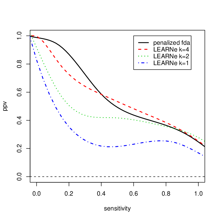
In the above simulations, we used when applying LEARNe to the simulated data, where is the subset size to search over in LEARNe. In these simulated data, it is known that the connection size is actually for each gene. Curiously, as shown in Figure 3, using results in much worse performances. As expected, if we use , the result is even worse. This shows that the performance of LEARNe depends critically on the size of subsets searched, which is in turn constrained by the computational resources available.
We demonstrate the performance of the our penalized functional model with the application to the cell cycle regulatory network of Saccharomyces cerevisiae. The dataset comes from (Spellman et al., 1998) which provides a comprehensive list of cell cycle regulated genes identified by time course expression analysis. We use the 18 time points of the alpha factor synchronized expression data. This dataset has been used widely for evaluating a wide variety of statistical models. Same as Nam et al. (2007), we consider 20 genes including 4 transcription factors known to be involved in regulatory functions during different stages of the cell cycle.
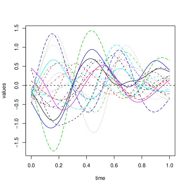
We apply our approach to this dataset. The temporal evolution of these 20 genes are shown in Figure 4 after B-spline smoothing of the expression data. To get a final model with data-based inference of network structure, we use the smoothing parameter selected by cross-validation with the same smoothing parameter for all 20 genes. The final result with the interactions between each gene and four transcription factor is shown in Table 1, and we compare the result with known interactions retrieved from the YEASTRACT database (Teixeira et al., 2006). For this submatrix, we get PPV=0.54 and sensitivity=0.80. Since all statistical models are merely mathematical approximations to the true world, it is plausible that automatically chosen model undersmoothes the coefficients matrix to provide a better fit to the data. One can also manually specify the smoothing parameter to achieved desired sparsity of the networks.
| ace2 | fkh1 | swi4 | swi5 | |
|---|---|---|---|---|
| ace2 | ||||
| fkh1 | ||||
| swi4 | ||||
| swi5 | ||||
| sic1 | ||||
| cln3 | ||||
| far1 | ||||
| cln2 | ||||
| cln1 | ||||
| clb6 | ||||
| clb5 | ||||
| gin4 | ||||
| swe1 | ||||
| clb4 | ||||
| clb2 | ||||
| clb1 | ||||
| tem1 | ||||
| apc1 | ||||
| spo12 | ||||
| cdc20 |
4 Discussion
We described a new algorithm for network construction using time course expression data. The algorithm is based on functional data analysis with connection coefficients regularized by the lasso penalty. This is a very powerful approach that makes inference for large networks possible due to the efficient optimization procedures previously proposed.
Our new algorithm provides several advantages over some previous approaches. First, it achieves noise reduction by regarding the expression data as continuous curves. High noise contained in the expression data usually disturbs inferences when one uses finite difference to approximate derivatives in the model. Second, the fitting procedure can be made fully automatic with little intervention from the user. The parameters in the model can be chosen using well studied statistical techniques such as cross-validation. Third, the existing optimization procedure can efficiently infer the network structure with the whole regularization path for the coefficients simultaneously and thus makes inference of large networks feasible.
It is well known that biological side information can reduce the number of false positives and false negatives. It would be interesting to take into account such information in future work. For example, prior knowledge on the interactions of genes can be incorporated into the smoothing parameter so that different interaction coefficients can be penalized differently, resulting in adaptive lasso penalty (Zou, 2006). We expect this strategy will achieve desired improvement on network prediction.
Funding
This research was funded by Singapore Ministry of Education Tier 1 SUG.
Acknowledgement
The author thanks Dr. Dougu Nam for providing the MATLAB code for LEARNe.
References
- Bansal et al. (2006) Bansal, M., Della Gatta, G., and di Bernardo, D. (2006). Inference of gene regulatory networks and compound mode of action from time course gene expression profiles. Bioinformatics, 22(7), 815–822.
- Chen et al. (2005) Chen, K. C., Wang, T. Y., Tseng, H. H., Huang, C. Y. F., and Kao, C. Y. (2005). A stochastic differential equation model for quantifying transcriptional regulatory network in saccharomyces cerevisiae. Bioinformatics, 21(12), 2883–2890.
- Efron et al. (2004) Efron, B., Hastie, T., Johnstone, I., and Tibshirani, R. (2004). Least angle regression. Annals of Statistics, 32(2), 407–451.
- Friedman (2004) Friedman, N. (2004). Inferring cellular networks using probabilistic graphical models. Science, 303(5659), 799–805.
- Gardner et al. (2003) Gardner, T. S., di Bernardo, D., Lorenz, D., and Collins, J. J. (2003). Inferring genetic networks and identifying compound mode of action via expression profiling. Science, 301(5629), 102–105.
- Hirose et al. (2008) Hirose, O., Yoshida, R., Imoto, S., Yamaguchi, R., Higuchi, T., Charnock-Jones, D. S., Print, C., and Miyano, S. (2008). Statistical inference of transcriptional module-based gene networks from time course gene expression profiles by using state space models. Bioinformatics, 24(7), 932–942.
- Nam et al. (2007) Nam, D., Yoon, S. H., and Kim, J. F. (2007). Ensemble learning of genetic networks from time-series expression data. Bioinformatics, 23(23), 3225–3231.
- Ramsay and Silverman (2005) Ramsay, J. O. and Silverman, B. W. (2005). Functional data analysis. Springer series in statistics. Springer, New York, 2nd edition.
- Rosset and Zhu (2007) Rosset, S. and Zhu, J. (2007). Piecewise linear regularized solution paths. Annals of Statistics, 35(3), 1012–1030.
- Spellman et al. (1998) Spellman, P. T., Sherlock, G., Zhang, M. Q., Iyer, V. R., Anders, K., Eisen, M. B., Brown, P. O., Botstein, D., and Futcher, B. (1998). Comprehensive identification of cell cycle-regulated genes of the yeast saccharomyces cerevisiae by microarray hybridization. Molecular Biology of the Cell, 9(12), 3273–3297.
- Teixeira et al. (2006) Teixeira, M. C., Monteiro, P., Jain, P., Tenreiro, S., Fernandes, A. R., Mira, N. P., Alenquer, M., Freitas, A. T., Oliveira, A. L., and Sa-Correia, I. (2006). The yeastract database: a tool for the analysis of transcription regulatory associations in saccharomyces cerevisiae. Nucleic Acids Research, 34, D446–D451.
- Tibshirani (1996) Tibshirani, R. (1996). Regression shrinkage and selection via the lasso. Journal of the Royal Statistical Society Series B-Methodological, 58(1), 267–288.
- Yu et al. (2004) Yu, J., Smith, V. A., Wang, P. P., Hartemink, A. J., and Jarvis, E. D. (2004). Advances to bayesian network inference for generating causal networks from observational biological data. Bioinformatics, 20(18), 3594–3603.
- Zou (2006) Zou, H. (2006). The adaptive lasso and its oracle properties. Journal of the American Statistical Association, 101(476), 1418–1429.