A 3-manifold complexity via immersed surfaces00footnotetext: This research has been supported by the grant “Ennio De Giorgi” (2007-2008) from the Department of Mathematics of the University of Salento.
Abstract
We define an invariant, which we call surface-complexity, of closed 3-manifolds by means of Dehn surfaces. The surface-complexity of a manifold is a natural number measuring how much the manifold is complicated. We prove that it fulfils interesting properties: it is subadditive under connected sum and finite-to-one on -irreducible manifolds. Moreover, for -irreducible manifolds, it equals the minimal number of cubes in a cubulation of the manifold, except for the sphere , the projective space and the lens space , which have surface-complexity zero. We will also give estimations of the surface-complexity by means of triangulations, Heegaard splittings, surgery presentations and Matveev complexity.
Keywords
3-manifold, complexity, immersed surface, cubulation.
MSC (2000)
57M27 (primary), 57M20 (secondary).
Introduction
The problem of filtering closed 3-manifolds in order to study them systematically has been approached by many mathematicians. The aim is to find a function from the class of closed 3-manifolds to the set of natural numbers. The number associated to a closed 3-manifold should be a measure of how much the manifold is complicated. For closed surfaces, this can be achieved by means of genus. For closed 3-manifolds, the problem has been studied very much and many possible functions has been found. For example, the Heegaard genus, the Gromov norm, the Matveev complexity have been considered.
All these functions fulfil many properties. For instance, they are additive under connected sum. However, some of them have drawbacks. The Heegaard genus and the Gromov norm are not finite-to-one, while the Matveev complexity is. Hence, in order to carry out a classification process, the latter one is more suitable than the former ones. The Matveev complexity is also a natural measure of how much the manifold is complicated, because if a closed 3-manifold is -irreducible and different from the sphere , the projective space and the Lens space , then its Matveev complexity is the minimum number of tetrahedra in a triangulation of the manifold (the Matveev complexity of , and is zero). Such functions could also be tools to give proofs by induction. For instance, the Heegaard genus was used by Rourke to prove by induction that every closed orientable 3-manifold is the boundary of a compact orientable 4-manifold [15].
The aim of this paper is to define another function (we will call surface-complexity) from the class of closed 3-manifolds to the set of natural numbers, to prove that it fulfils some properties, to give bounds for it, and to start an enumeration process (we will give a complete list of closed 3-manifolds with complexity one in a subsequent paper [3]).
In [19] Vigara used triple points of particular transverse immersions of connected closed surfaces to define the triple point spectrum of a 3-manifold. The definition of the surface-complexity is similar to Vigara’s one, but it has the advantage of being more flexible. This flexibility will allow us to prove many properties fulfilled by the surface-complexity.
We now sketch out the definition and the results of this paper. The surface-complexity of a closed 3-manifold will be defined by means of quasi-filling Dehn surfaces (i.e. images of transverse immersions of closed surfaces that divide the manifold into balls).
- Definition.
-
The surface-complexity of a closed 3-manifold is the minimal number of triple points of a quasi-filling Dehn surface of .
Three properties we will prove are the following ones.
- Finiteness.
-
For any integer there exists only a finite number of connected closed -irreducible 3-manifolds having surface-complexity .
- Naturalness.
-
The surface-complexity of a connected closed -irreducible 3-manifold , different from , and , is the minimal number of cubes in a cubulation of . The surface complexity of , and is zero.
- Subadditivity.
-
The complexity of the connected sum of closed 3-manifolds is less than or equal to the sum of their complexities.
The naturalness property will follow from the features of minimal quasi-filling Dehn surfaces of connected closed -irreducible 3-manifolds, where minimal means “with a minimal number of triple points”. We will call a quasi-filling Dehn surface of a 3-manifold filling, if its singularities induce a cell-decomposition of . The cell-decomposition dual to a filling Dehn-surface of is actually a cubulation of . Hence, in order to prove the naturalness property, we will prove that every connected closed -irreducible 3-manifold, different from , and , has a minimal filling Dehn surface. We point out that not all the minimal quasi-filling Dehn surfaces of -irreducible 3-manifolds are indeed filling. However, they can be all constructed starting from filling ones (except for , and , for which non-filling ones must be used) and applying a simple move, we will call bubble-move.
The surface-complexity is related to the Matveev complexity. Indeed, if is a connected closed -irreducible 3-manifold different from and , the double inequality holds, where denotes the Matveev complexity of . For the sake of completeness, we recall that we have , , and .
The two inequalities above give also estimates of the surface-complexity. In general, an exact calculation of the surface-complexity of a closed 3-manifold is very difficult, however it is relatively easy to estimate it. More precisely, it is quite easy to give upper bounds for it, because constructing a quasi-filling Dehn surface of the manifold with the appropriate number of triple points suffices. With this technique, we will give upper bounds for the surface-complexity of a closed 3-manifold starting from a triangulation, a Heegaard splitting and a surgery presentation on a framed link (in ) of it.
In the Appendix, we will state some results on closed 3-manifolds with surface-complexity one and we will give some examples. However, we will postpone the theoretical proof of these results and the classification of the closed 3-manifolds with surface-complexity one to a subsequent paper [3]. For the sake of completeness, in the Appendix we will also give a brief description of what happens in the 2-dimensional case. We plan to cope with the 4-dimensional case in a subsequent paper.
1 Definitions
Throughout this paper, all 3-manifolds are assumed to be connected and closed. By , we will always denote such a (connected and closed) 3-manifold. Using the Hauptvermutung, we will freely intermingle the differentiable, piecewise linear and topological viewpoints.
Dehn surfaces
A subset of is said to be a Dehn surface of [13] if there exists an abstract (possibly non-connected) closed surface and a transverse immersion such that .
Let us fix for a while a transverse immersion (hence, is a Dehn surface of ). By transversality, the number of pre-images of a point of is 1, 2 or 3; so there are three types of points in , depending on this number; they are called simple, double or triple, respectively. Note that the definition of the type of a point does not depend on the particular transverse immersion we have chosen. In fact, the type of a point can be also defined by looking at a regular neighbourhood (in ) of the point, as shown in Fig. 1. The set of triple points is denoted by ; non-simple points are called singular and their set is denoted by .


 Simple
point
Double
point
Triple
point
Simple
point
Double
point
Triple
point
From now on, in all figures, triple points are always marked by thick dots and the singular set is also drawn thick.
Remark 1.
The topological type of the abstract surface is determined unambiguously by .
(Quasi-)filling Dehn surfaces
A Dehn surface of will be called quasi-filling if is made up of balls. Moreover, is called filling [12] if its singularities induce a cell-decomposition of ; more precisely,
- •
,
- •
is made up of intervals (called edges),
- •
is made up of discs (called regions),
- •
is made up of balls (i.e. is quasi-filling).
Since is connected and is made up of (disjoint) balls, the quasi-filling Dehn surface is connected. Consider a small regular neighbourhood of in , then is made up of balls whose closures are disjoint and can be obtained from by filling up its boundary components with balls. Moreover, we have that minus some balls, i.e. , collapses to .
Remark 2.
Suppose is a surface (i.e. ). Then the boundary of of in is a two-fold covering of . Since the boundary of is made up of spheres and is connected, is the sphere or the projective plane . Therefore, is the sphere or the projective space , respectively.
Let us give some other examples. Two projective planes intersecting along a loop non-trivial in both of them form a quasi-filling Dehn surface of , which will be called double projective plane and denoted by . The sphere intersecting a torus (resp. a Klein bottle) along a loop is a quasi-filling Dehn surface of (resp. ) without triple points. The quadruple hat (i.e. a disc whose boundary is glued four times along a circle) is a quasi-filling Dehn-surface of the lens-space without triple points. If we identify the sphere with , the three coordinate planes in , with added, form a filling Dehn surface of with two triple points: and .
It is by now well-known that a filling Dehn surface determines up to homeomorphism and that every has standard filling Dehn surfaces (see, for instance, Montesinos-Amilibia [12] and Vigara [18], see also [2]). It is not clear how any two standard filling Dehn spheres of the same are related to each other. There are only partial results; for instance, we provided in [2] a finite calculus for nullhomotopic filling Dehn spheres, deducing it from another one, described by Vigara [19], which has been derived from the more general Homma-Nagase calculus [8, 9] (see also Hass and Hughes [7] and Roseman [14]).
Abstract filling Dehn surfaces
A filling Dehn surface of is contained . However, we can think of if as an abstract cell complex. For the sake of completeness, we point out that the abstract cell complex determines (and the abstract surface such that where ) up to homeomorphism. The proof of this fact is quite easy (and not strictly connected with the aim of this paper), so we leave it to the reader.
Surface-complexity
The surface-complexity of can now be defined as the minimal number of triple points of a quasi-filling Dehn surface of . More precisely, we give the following.
Definition 3.
The surface-complexity of is equal to if possesses a quasi-filling Dehn surface with triple points and has no quasi-filling Dehn surface with less than triple points. In other words, is the minimum of over all quasi-filling Dehn surfaces of .
We will classify the 3-manifolds having surface-complexity zero in the following section. At the moment, we can only say that , , , and have surface-complexity zero, because we have seen above that they have quasi-filling Dehn surfaces without triple points.
Triple point spectrum
For the sake of completeness, we give also Vigara’s definition of the triple point spectrum [19]. The triple point spectrum of is a sequence of integers , with , such that is the minimal number of triple points of a filling Dehn surface with genus of .
2 Minimality and finiteness
A quasi-filling Dehn surface of is called minimal if it has a minimal number of triple points among all quasi-filling Dehn surfaces of , i.e. .
Theorem 4.
Let be a (connected and closed) -irreducible 3-manifold.
- •
If , then is the sphere , the projective space or the lens space .
- •
If , then has a minimal filling Dehn surface.
Proof.
Let be a minimal quasi-filling Dehn surface of . If we have (i.e. is a surface), by virtue of Remark 2, we have that is the sphere or the projective space .
Then, we suppose . We will first prove that has a quasi-filling Dehn surface such that is made up of discs. In fact, suppose there exists a component of that is not a disc. contains a non-trivial orientation preserving (in ) simple closed curve . Consider a strip contained in a small regular neighbourhood of in such that and . (Note that is an annulus or a Möbius strip depending on whether is orientation preserving in or not.) Since is made up of balls, we can fill up with one or two discs disjoint from getting a sphere or a projective plane (depending on whether is an annulus or a Möbius strip). Note that both the sphere and the projective plane are transversely orientable, hence the second case cannot occur (because is -irreducible). In the first case, since is -irreducible, the sphere found bounds a ball, say . Since is a ball and is a simple closed curve, we can replace the portion of contained in with a disc, getting a new quasi-filling Dehn surface of . Note that the Euler characteristic of the component of containing has increased, that no new non-disc component has been created and that the number of triple points has not changed. Hence, by repeatedly applying this procedure, we eventually get a quasi-filling Dehn surface, say , of such that is made up of discs.
Since is connected and is made up of discs, we have that is also connected. If we have (i.e. is not empty), cannot contain circles and hence is filling (i.e. has a minimal filling Dehn surface). Otherwise, if we have (i.e. is empty), is made up of one circle. Since is made up of discs, the Dehn surface is completely determined by the regular neighbourhood of in . This neighbourhood depends on how the germs of disc are interchanged along the curve . Among all possibilities we must rule out those not yielding a quasi-filling Dehn surface, hence only three ones must be taken into account (up to symmetry):
- •
two spheres intersecting along the circle which form a Dehn surface of ;
- •
the double projective plane which is a Dehn surface of ;
- •
the four-hat which is a Dehn surface of .
The proof is complete. ∎
Since there is a finite number of filling Dehn surfaces having a fixed number of triple points, we have the following corollary of Theorem 4.
Corollary 5.
For any integer there exists only a finite number of (connected and closed) -irreducible 3-manifolds having surface-complexity .
2.1 Minimal quasi-filling Dehn surfaces
Not all the minimal quasi-filling Dehn surfaces of -irreducible 3-manifolds are indeed filling. However, they can be all constructed starting from filling ones (except for , and , for which non-filling ones must be used) and applying a simple move. The move acts on quasi-filling Dehn surfaces near a simple point as shown in Fig. 2 and it is called bubble-move.

Note that the result of applying a bubble-move to a quasi-filling Dehn surface of is a quasi-filling Dehn surface of , but the result of applying a bubble-move to a filling Dehn-surface is not a filling Dehn-surface. Note also that the bubble-move increases (by two) the number of connected components of . If a quasi-filling Dehn surface is obtained from a quasi-filling Dehn surface by repeatedly applying bubble-moves, we will say that is derived from . Note that if is a quasi-filling Dehn surface of and is derived from , than is a quasi-filling Dehn surface of .
Theorem 4 can be improved by means of a slightly subtler analysis.
Lemma 6.
Let be a minimal quasi-filling Dehn surface of the sphere and let be a closed disc disjoint from the singular set of . Then is derived from a sphere by means of bubble-moves not involving .
Proof.
Since the surface complexity of is zero, the number of triple points of is zero and hence the connected components of , if there is any, are simple closed curves. If we have (i.e. is a surface), by virtue of Remark 2, we have that is the sphere . Then, we will suppose and we will prove the statement by induction on the number of connected components of .
Suppose that has one connected component. We will firstly prove that is made up of discs. In fact, suppose by contradiction that there exists a component of that is not a disc. contains a non-trivial orientation preserving (in ) simple closed curve . Consider a strip contained in a small regular neighbourhood of in such that and . Note that is an annulus because is orientation preserving in . Since is made up of balls, we can fill up the annulus with two discs disjoint from getting a sphere. This sphere bounds two balls, say and . Since does not intersect the disconnecting sphere, we have that is wholly contained either in or in (we can assume in ). Hence, is a surface cutting up into two balls, whose boundaries contain . Since has only one boundary component (), it is a disc and hence is trivial in , a contradiction. We have proved that is made up of discs. Since is connected and does not contain triple points, it is a circle and the Dehn surface is completely determined by the regular neighbourhood of in . This neighbourhood depends on how the germs of disc are interchanged along the curve . Among all possibilities, only one yields a quasi-filling Dehn surface of : more precisely, is composed of two spheres intersecting along the circle . We conclude by noting that is derived from the sphere by means of a bubble-move not involving .
Finally, suppose that has components with and suppose that the statement is true for all minimal quasi-filling Dehn surfaces of whose singular set has less than components. Consequently, is not connected and there is a connected component of that is not a disc. This component contains a non-trivial orientation preserving (in ) simple closed curve disjoint from the disc . As done above, we can construct a sphere intersecting along . Cutting up by this sphere, we obtain two balls (say and ) both of which contain some components of . Note that the disc is wholly contained either in or in (we can assume in ). Consider now . If we fill up with a disc (say ) by gluing it along , we obtain a minimal quasi-filling Dehn surface of such that has less than components. We can apply the inductive hypothesis and we have that is derived from a sphere by means of bubble-moves not involving . Since these moves do not involve the disc , we can repeat these moves on obtaining a minimal quasi-filling Dehn surface of such that has less than components. Note that all moves do not involve the disc . By applying again the inductive hypothesis, we obtain that is derived from a sphere by means of bubble-moves not involving . Summing up is derived from a sphere by means of bubble-moves not involving . This concludes the proof. ∎
We are now able to prove the theorem that tells us how to construct all minimal quasi-filling Dehn surfaces starting from the filling ones (except for , and , for which non-filling ones must be used).
Theorem 7.
Let be a minimal quasi-filling Dehn surface of a (connected and closed) -irreducible 3-manifold .
- •
If , one of the following holds:
- –
is the sphere and is derived from the sphere ,
- –
is the projective space and is derived from the projective plane or from the double projective plane ,
- –
is the lens space and is derived from the four-hat.
- –
- •
If , then is derived from a minimal filling Dehn surface of .
Proof.
The scheme of the proof is the same as that of Theorem 4. Hence, we will often refer to the proof of Theorem 4 also for notation.
Let be a minimal quasi-filling Dehn surface of . If we have (i.e. is a surface), by virtue of Remark 2, we have that is the sphere or the projective plane , and that is the sphere or the projective space , respectively.
Then, we suppose . We will first prove that is derived from a (minimal) quasi-filling Dehn surface of such that either is made up of discs or is a surface. In fact, suppose there exists a component of that is not a disc. contains a non-trivial orientation preserving (in ) simple closed curve . As done in the proof of Theorem 4, we can construct a sphere contained in such that . Since is -irreducible, the sphere found bounds a ball, say . Consider now and . If we fill up with a disc by gluing it along , we obtain a minimal quasi-filling Dehn surface of . Analogously, if we fill up with a disc (say ) by gluing it along , we obtain a minimal quasi-filling Dehn surface of . By virtue of Lemma 6, is derived from a sphere by means of bubble-moves not involving . These moves can by applied to because they do not involve . Note that the Euler characteristic of the component of containing has increased, that no new non-disc component has been created and that the number of triple points has not changed. Hence, by repeatedly applying this procedure, we eventually get a (minimal) quasi-filling Dehn surface of from which is derived and such that either is made up of discs or is a surface.
If is a surface, by virtue of Remark 2, is either or , and is or , respectively; therefore, we have done. Then, we suppose that is made up of discs. Since is connected, we have that is also connected. If we have (i.e. is not empty), cannot contain circles and hence is filling (i.e. is derived from a minimal filling Dehn surface of ). Otherwise, if we have (i.e. is empty), is made up of one circle. Since is made up of discs, the Dehn surface is completely determined by the regular neighbourhood of in . This neighbourhood depends on how the germs of disc are interchanged along the curve . Among all possibilities we must rule out those not yielding a quasi-filling Dehn surface, hence only three ones must be taken into account (up to symmetry):
- •
two spheres intersecting along the circle which form a Dehn surface of ;
- •
the double projective plane which is a Dehn surface of ;
- •
the four-hat which is a Dehn surface of .
Note that in the first case is derived from the sphere . Therefore, is derived from , or the four hat. The proof is complete. ∎
3 Cubulations
A cubulation of is a cell-decomposition of such that
- •
each 2-cell (called face) is glued along 4 edges,
- •
each 3-cell (called cube) is glued along 6 faces arranged like the boundary of a cube.
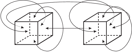
Note that self-adjacencies and multiple adjacencies are allowed. In Fig. 3 we have shown a cubulation of the 3-dimensional torus with two cubes (the identification of each pair of faces is the obvious one, i.e. the one without twists).
The following construction is well-known (see [1, 6, 4], for instance). Let be a cubulation of a closed 3-manifold; consider, for each cube of , the three squares shown in Fig. 4; the subset of obtained by gluing together all these squares is a filling Dehn surface of (up to isotopy, we can suppose that the squares fit together through the faces).

Conversely, a cell-decomposition can be constructed from a filling Dehn surface of by considering an abstract cube for each triple point of and by gluing the cubes together along the faces (the identification of each pair of faces is chosen by following the four germs of regions adjacent to the respective edge of ); the cell-decomposition just constructed is indeed a cubulation of . The cubulation and the filling Dehn surface constructed in such a way are said to be dual to each other.
An obvious corollary of Theorem 4 is the following result.
Corollary 8.
The surface-complexity of a (connected and closed) -irreducible 3-manifold, different from , and , is equal to the minimal number of cubes in a cubulation of .
4 Subadditivity
An important feature of a complexity function is to behave well with respect to the cut-and-paste operations. In this section, we will prove that the surface-complexity is subadditive under connected sum. We do not know whether it is indeed additive.
Theorem 9.
The complexity of the connected sum of (connected and closed) 3-manifolds is less than or equal to the sum of their complexities.
Proof.
In order to prove the theorem, it is enough to prove the statement in the case where the number of the manifolds involved in the connected sum is two. Hence, if we call and the two manifolds, we need to prove that . Let (resp. ) be a quasi-filling Dehn surface of (resp. ) with (resp. ) triple points. If the balls we remove to obtain the connected sum are disjoint from the ’s, we can suppose that and are embedded also in the connected sum . All the components of are balls except one that is a product ; see Fig. 5-left.

We modify as shown in Fig. 5-right, getting a Dehn surface, say . The complement is made up of the same balls as before (up to isotopy), a new small ball and a product (which is indeed a ball). Therefore, is a quasi-filling Dehn surface of . Since has triple points, we have . ∎
5 Estimations
5.1 Matveev complexity
The Matveev complexity [10] of a closed 3-manifold is defined using simple spines. A polyhedron is simple if the link of each point of can be embedded in the 1-skeleton of the tetrahedron. The points of whose link is the whole 1-skeleton of the tetrahedron are called vertices. A sub-polyhedron of is a spine of if is a ball. The Matveev complexity of is the minimal number of vertices of a simple spine of . The Matveev complexity is a natural measure of how much the manifold is complicated, because if is -irreducible and different from the sphere , the projective space and the Lens space , then its Matveev complexity is the minimum number of tetrahedra in a triangulation of it (the Matveev complexity of , and is zero). A simple spine of is standard if it is purely 2-dimensional and its singularities induce a cell-decomposition of . The dual cellularization of a standard spine of is a one-vertex triangulation of , see [11].
The Matveev complexity is related to the surface-complexity. Before describing more precisely this relation, we describe two constructions allowing us to create standard spines (or one-vertex triangulations, by duality) from filling Dehn surfaces (or cubulations, by duality), and vice versa.
Let be a one-vertex triangulation of . Consider, for each tetrahedron of , the four triangles shown in Fig. 6.

The subset of obtained by gluing together all these triangles is a Dehn surface of with triple points (up to isotopy, we can suppose that the triangles fit together through the faces). It is very easy to prove that is filling, so we leave it to the reader. The construction just described is the dual counterpart of the well-known construction consisting in dividing a tetrahedron into four cubes [17, 5, 6].
Conversely, let be a cubulation of . Consider, for each cube of , the five tetrahedra shown in Fig. 7.

The idea is to glue together these “bricks” (each of which is made up of five tetrahedra) by following the identifications of the faces of . Note that the faces of the cubes are divided by diagonals into two triangles and that it may occur that these pairs of triangles do not match each other. If they do not match each other, we insert a tetrahedron between them as shown in Fig. 8.

Eventually, we get a triangulation of with tetrahedra for each cube of and at most one tetrahedron for each face of . Since the number of faces of a cubulation is thrice the number of cubes, we have that the triangulation we have constructed has at most tetrahedra.
We note that there are two different identifications of the abstract “brick” with each cube, so there are possibilities for the identifications with the cubes of . Some of them may need less insertions of tetrahedra (for matching the pairs of triangles in the faces of ) than others. Hence, optimal choices may lead to a triangulation of with tetrahedra or few more.
The two constructions above and the list of the (connected and closed) -irreducible 3-manifolds with or obviously imply the following.
Theorem 10.
Let be a (connected and closed) -irreducible 3-manifold different from and ; then we have
Moreover, we have , , and .
5.2 Other estimations
In general, calculating the surface-complexity of is very difficult, however it is relatively easy to estimate it. More precisely, it is quite easy to give upper bounds for it. If we construct a quasi-filling Dehn surface of , the number of triple points of is an upper bound for the surface-complexity of . Afterwards, the (usually difficult) problem of proving the sharpness of this bound arises.
We can construct quasi-filling Dehn surfaces of from many presentations of and hence we obtain estimates from many presentations of . We use here three presentations: triangulations, Heegaard splittings and Dehn surgery.
We have already constructed a filling Dehn surface of from a one-vertex triangulation of in Section 5.1. The same construction applies to any triangulation of , yielding the following result.
Theorem 11.
Suppose a closed 3-manifold has a triangulation with tetrahedra. Then, we have .
Proof.
Let be the triangulation of with tetrahedra. Consider, for each tetrahedron of , the four triangles shown in Fig. 6. The subset of obtained by gluing together all these triangles is a Dehn surface of with triple points. It is very easy to prove that is filling, so we leave it to the reader. ∎
Theorem 12.
Suppose is a Heegaard splitting of a closed 3-manifold such that the meridians of the handlebody intersect those of transversely in points. Then, we have .
Proof.
Let be the number of meridians of and be the common boundary of and . Let (resp. ), with , be the meridians of (resp. ).
Let us suppose at first that each meridian of intersects at least one of , and vice versa. Let us call be the disc bounded by in . The boundary of a small regular neighbourhood of a disc is a sphere (say ) intersecting transversely along two loops parallel to , see Fig. 9.

The union of and the spheres is a Dehn surface, say ; we show it near an intersection point between a meridian of and one of in Fig. 10.

We prove now that is quasi-filling. Since is contained in and since the role of the two handlebodies is symmetrical, it is enough to prove that is made up of balls. The spheres divide into balls, because the discs do and each is made up of two discs parallel to . Moreover, the spheres divide these balls into smaller balls, because each meridian of intersects at least one of . Each point of intersection of two meridians yields 4 triple point (see Fig. 10), hence the number of triple points of is . Therefore, we have proved that if each meridian of intersects at least one of , and vice versa, then we have .
Suppose now that some meridian of does not intersect any of (the case of a meridian of is symmetrical). We can suppose, without loss of generality, that this meridian is . This Heegaard splitting is reducible. A loop in parallel to bounds in fact a disc both in and in . Let us call these discs and , respectively. We can suppose that is parallel to . The disc does not disconnect , therefore the sphere does not disconnect . Hence, is the connected sum of (or ) and another manifold, say . Moreover, we can explicitly construct a Heegaard splitting of . Namely, the two handlebodies, say , are obtained by cutting along (for ); the gluing map coincides with the old one out of the two pairs of discs created in the boundary of by the cut and identifies the four discs in pairs. Moreover, we consider the class of meridians of made up of , with . In order to get a class of meridians of , we consider the meridians discarding one of them: in order to choose the one to discard, we look at the two spheres with holes obtained by cutting the boundary of along the meridians and we discard a that is adjacent to both spheres. Note that a good choice of the to discard may yield a decrease of the number of intersections between the meridians; however, we only know that the number of intersections between the meridians does not increase.
If now some meridian of does not intersect any of , or vice versa, then we repeat the procedure. Eventually, we have that is the connected sum of some copies of (and ) and another manifold . Moreover, we obtain that has a Heegaard splitting such that each meridian of a handlebody intersects at least one of the other handlebody. If there is no meridian, is the sphere and hence ; otherwise, we have constructed a quasi-filling Dehn surface of with 4 triple points for each intersection of the meridians of the Heegaard splitting of . The number of intersections cannot increase along the procedure, therefore we have . Since we have (and ), by virtue of Theorem 9, we have . The proof is complete. ∎
Remark 13.
In [11] the following is proven:
Suppose is a Heegaard splitting of a closed 3-manifold such that the meridians of the handlebody intersect those of transversely in points.
Suppose also that the closure of one of the components into which the meridians of and divide contains such points.
Then, we have .
We can use this result to improve the estimation of of Theorem 12 if the decomposition of into prime manifolds contains only -irreducible closed 3-manifolds different from . Let be the connected sum of -irreducible manifolds , such that no is . By virtue of the statement above, we have . Since the Matveev complexity is additive under connected sum, we have . Note that Theorem 10 implies for each . Then, by virtue of Theorem 9, we have .
Theorem 14.
Suppose is obtained by Dehn surgery along a framed link in (hence is orientable). Moreover, suppose has a projection such that the framing is the blackboard one, there are crossing points and there are components containing no overpass. Then, we have .
Proof.
The projection plane can be regarded as a subset of a sphere contained in . We add a cylinder for each arc of the projection, as shown in Fig. 11.

We connect these cylinders by a pair of intersecting cylinders for each crossing point, as shown in Fig. 12.

The result is a Dehn surface, say , contained in and made up of the sphere and some tori (namely, one torus for each component of ).
The complement of in is made up of balls and solid tori. More precisely, we have one torus for each component of and one more torus for each component containing no overpass: note indeed that if is the torus corresponding to one of these components, then is made up of two balls and two tori, both of which are not divided into balls by overpasses. In order to divide them, we add one small sphere for each component containing no overpass, as shown in Fig. 13, getting another Dehn surface, say .

Now, the complement of in is made up of some balls and one torus for each component of the link . Moreover, up to isotopy, we can suppose that the union of the tori is a regular neighbourhood of the link . Hence, the Dehn surface can be regarded as a Dehn surface in . Furthermore, the complement of in is also made up of some balls and one torus, say , for each component of the link .
In order to get a quasi-filling Dehn surface of , we will divide the tori into balls by adding spheres. For each torus , let be a curve giving the (blackboard) framing, disjoint from and lying above (with respect to the projection); see Fig. 14.

Moreover, consider a disc bounded in by the curve and consider the boundary of a small regular neighbourhood of the disc, say . Each surface is a sphere intersecting along two curves (see Fig. 15).

We add the spheres to and we call the result . The complement of the Dehn surface in is made up of balls, so is a quasi-filling Dehn surface of . Moreover, has 8 triple points for each crossing of the projection of (see Fig. 15) and 4 triple points for each component of containing no overpass (see Fig. 13). The proof is complete. ∎
Remark 15.
If the framing is not the blackboard one, some curls must be added to the curves , as shown in Fig. 16.

However, a simple generalisation of the procedure shown in the proof of Theorem 14 yields an upper bound for surface-complexity by means of non-blackboard framings, where the wirthe (i.e. the blackboard framing) appears. More precisely, with the notation of Theorem 14, if and are, respectively, the framing and the wirthe of the -th component of the link, then we have .
Appendix A Starting enumeration
We recall that there are eight important 3-dimensional geometries: six of them concern Seifert manifolds (, , , , Nil and ), one concerns Stallings manifolds (Sol) and the last is the hyperbolic one [16]. The geometry of a Seifert manifold is determined by two invariants of any of its fibrations, namely the Euler characteristic of the base orbifold and the Euler number of the fibration, according to Table 1.
Nil
Finally, we recall that non-orientable Seifert manifolds cannot have , i.e. cannot be of type , Nil and .
In a subsequent paper [3], we will prove the following.
Theorem 16.
- •
There are no -irreducible orientable closed 3-manifolds having surface-complexity one of type , , Sol, hyperbolic or non-geometric.
- •
There are -irreducible orientable closed 3-manifolds having surface-complexity one of type (e.g. the lens spaces , , , ) and (e.g. the 3-dimensional torus ).
- •
There are no -irreducible non-orientable closed 3-manifolds having surface-complexity one of type , hyperbolic or non-geometric.
- •
There are -irreducible non-orientable closed 3-manifolds having surface-complexity one of type (e.g. the trivial bundle over the Klein bottle ).
Appendix B The bidimensional case
Let be a connected closed surface. Let us denote by the disjoint union of circles . A subset of is said to be a Dehn loop of if there exists and a transverse immersion such that ; some examples are shown in Fig. 17.

There are only two types of points in : smooth points and crossing points (see Fig. 18). The set of crossing points is denoted by .

A Dehn loop of will be called quasi-filling if is made up of discs; it will be called filling if its singularities induce a cell-decomposition of : more precisely,
- •
,
- •
is made up of intervals,
- •
is made up of discs (i.e. is quasi-filling).
Note that the second condition is automatically satisfied once the other two are fulfilled. It can be easily shown that only the sphere and the projective plane have quasi-filling Dehn loops that are not filling, while all non-positive Euler characteristic surfaces have only filling Dehn loops; see Fig. 17. Each surface has a filling Dehn loop. However, as opposed to the 3-dimensional case, a filling Dehn loop does not determine ; in fact, the bouquet of two circles is a Dehn loop of the projective plane , the torus and the Klein bottle ; see Fig. 17.
We define the loop-complexity of a connected closed surface as the minimal number of crossing points of a quasi-filling Dehn loop of . The loop-complexity of the surface with Euler characteristic is , except for the sphere having loop complexity zero. In terms of the genus of the surface, we have:
- •
the loop-complexity of the sphere and of the projective plane is zero,
- •
the loop-complexity of the orientable genus- surface is ,
- •
the loop-complexity of the non-orientable genus- surface is .
Note that it is not true that the loop-complexity of the connected sum of two surfaces is at most the sum of their loop-complexities; for instance, we have while .
A cubulation of a connected closed surface (i.e. a cell-decomposition of such that each 2-cell, called square, is glued along 4 edges) can be constructed from a filling Dehn loop of by considering an abstract square for each crossing point of and by gluing the squares together along the edges. However, there are two possibilities for gluing two squares along an edge and the abstract polyhedron does not encode any information to choose the right one. (In some sense, this explains why a filling Dehn loop does not determine unambiguously one surface.) If we consider also the immersion of in the surface containing the Dehn loop , we can choose the right identifications and construct a cubulation of .
The converse construction can also be performed obtaining a filling Dehn loop of a connected closed surface from a cubulation of . These constructions tells us that is the minimal number of squares in a cubulation of , except for and whose loop-complexity is zero.
Acknowledgements
I would like to thank the Department of Mathematics of the University of Salento for the nice welcome and, in particular, Prof. Giuseppe De Cecco for his willingness.
References
- [1] I. R. Aitchison – S. Matsumotoi – J. H. Rubinstein, Immersed surfaces in cubed manifolds, Asian J. Math. 1 (1997), no. 1, 85–95.
- [2] G. Amendola, Invariants of closed 3-manifolds via nullhomotopic filling Dehn spheres, preprint, http://arxiv.org/abs/0707.3226, 33 pp.
- [3] G. Amendola, The closed 3-manifolds obtained from one cube, in preparation.
- [4] E. K. Babson – C. S. Chan, Counting faces of cubical spheres modulo two, Discrete Math. 212 (2000), no. 3, 169–183.
- [5] N. P. Dolbilin – M. A. Shtan′ko – M. I. Shtogrin, Cubic manifolds in lattices, Izv. Ross. Akad. Nauk Ser. Mat. 58 (1994), no. 2, 93–107; translation in Russian Acad. Sci. Izv. Math. 44 (1995), no. 2, 301–313.
- [6] L. Funar, Cubulations, immersions, mappability and a problem of Habegger, Ann. Sci. École Norm. Sup. (4) 32 (1999), no. 5, 681–700.
- [7] J. Hass – J. Hughes, Immersions of surfaces in 3-manifolds, Topology 24 (1985), no. 1, 97–112.
- [8] T. Homma – T. Nagase, On elementary deformations of maps of surfaces into 3-manifolds. I, Yokohama Math. J. 33 (1985), no. 1-2, 103–119.
- [9] T. Homma – T. Nagase, On elementary deformations of maps of surfaces into 3-manifolds. II, Topology and computer science (Atami, 1986), 1–20, Kinokuniya, Tokyo, 1987.
- [10] S. V. Matveev, The theory of the complexity of three-dimensional manifolds, Akad. Nauk Ukrain. SSR Inst. Mat. Preprint (1988), no. 13, 32 pp.
- [11] S. V. Matveev, “Algorithmic topology and classification of 3-manifolds,” Algorithms and Computation in Mathematics, 9. Springer-Verlag, Berlin, 2003. xii+478 pp.
- [12] J. M. Montesinos-Amilibia, Representing 3-manifolds by Dehn spheres, Mathematical contributions: volume in honor of Professor Joaquín Arregui Fernández, 239–247, Homen. Univ. Complut., Editorial Complutense, Madrid, 2000.
- [13] C. D. Papakyriakopoulos, On Dehn’s lemma and the asphericity of knots, Ann. of Math. (2) 66 (1957), 1–26.
- [14] D. Roseman, Reidemeister-type moves for surfaces in four-dimensional space, Knot theory (Warsaw, 1995), 347–380, Banach Center Publ., 42, Polish Acad. Sci., Warsaw, 1998.
- [15] C. Rourke, A new proof that is zero, J. London Math. Soc. (2) 31 (1985), no. 2, 373–376.
- [16] P. Scott, The geometries of -manifolds, Bull. London Math. Soc. 15 (1983), 401-487.
- [17] M. A. Shtan′ko – M. I. Shtogrin, Embedding cubic manifolds and complexes into a cubic lattice, Uspekhi Mat. Nauk 47 (1992), no. 1 (283), 219–220; translation in Russian Math. Surveys 47 (1992), no. 1, 267–268.
- [18] R. Vigara, A new proof of a theorem of J. M. Montesinos, J. Math. Sci. Univ. Tokyo 11 (2004), no. 3, 325–351.
- [19] R. Vigara, A set of moves for Johansson representation of 3-manifolds, Fund. Math. 190 (2006), 245–288.
Department of Mathematics
University of Salento
Palazzo Fiorini, Via per Arnesano
I-73100 Lecce, Italy
amendola@mail.dm.unipi.it