跳到论文正文
W Papers独立论文阅读器 arXiv:0804.0686 论文正文 计算阅读时间 · 0%
引用这篇论文根据当前论文元数据生成,正式投稿前建议核对。


License: CC Zero
arXiv:0804.0686v1 [quant-ph] 04 Apr 2008

Discrimination of two channels by adaptive methods and its application to quantum system

Masahito Hayashi ††thanks: M. Hayashi is with Graduate School of Information Sciences, Tohoku University, Aoba-ku, Sendai, 980-8579, Japan (e-mail: hayashi@math.is.tohoku.ac.jp)
Abstract

The optimal exponential error rate for adaptive discrimination of two channels is discussed. In this problem, adaptive choice of input signal is allowed. This problem is discussed in various settings. It is proved that adaptive choice does not improve the exponential error rate in these settings. These results are applied to quantum state discrimination.

Index Terms: 
Simple hypothesis testing, Channel, Discrimination, Quantum state, One-way LOCC, Active learning, Experimental design, Stein’s lemma, Chernoff bound, Hoeffding bound, Han-Kobayashi bound

I Introduction

Discriminating two distributions is treated as a fundamental problem in the field of statistical inference. This problem can be regarded as simple hypothesis testing because both hypotheses consist of a single distribution. Many researchers, Stein, Chernoff[3], Hoeffding[16], and Han-Kobayashi[10] have studied the asymptotic behavior when the number nn of identical and independent observations is sufficiently large. They formulated a simple hypothesis testing/discrimination of two distributions as an optimization problem and derived the respective optimum value, e.g., the optimal exponential error rate. We call these optimum values the Stein bound, the Chernoff bound, the Hoeffding bound, and the Han-Kobayashi bound, respectively. Han [8, 9] later extended these results to the discrimination of two general sequences of distributions, including the Markovian case. Nagaoka-Hayashi [21] simplified Han’s discussion and generalized Han’s extension of the Han-Kobayashi bound.

In the present paper, we consider another extension of the above results. That is, we extend the above results to the discrimination of two (classical) channels, in which two probabilistic transition matrices are given. Such a problem has appeared in Blahut[2]. In this problem, the number of applications of this channel is fixed to a given constant nn, and we can choose appropriate inputs for this purpose. In this case, we assume that the given channel is memoryless. If we use the same input to all applications of the given channel, the nn output data obeys an identical and independent distribution. This property holds even if we choose the input randomly based on the same distribution on input signals. This strategy is called the non-adaptive method. In particular, when the same input is applied to all channels, it is called the deterministic non-adaptive method. If the input is determined stochastically, it is called the stochastic non-adaptive method, which was treated by Blahut[2]. In the non-adaptive method, our task is choosing the optimal input for distinguishing two channels most efficiently. In the present paper, we assume that we can choose the kk-th input signal based on the preceding k−1k-1 output data. This strategy is called the adaptive method, which is the main focus of the present paper. In the parameter estimation, such an adaptive method improves estimation performance. That is, in the one-parameter estimation, the asymptotic estimation error is bounded by the inverse of the optimum Fisher information. However, if we do not apply the adaptive method, it is generally impossible to realize the optimum Fisher information in all points at the same time. It is known that the adaptive method realizes the optimum Fisher information in all points[13, 7]. Therefore, one may expect that the adaptive method improves the performance of discriminating two channels.

As our main result, we succeeded in proving that the adaptive method cannot improve the non-adaptive method in the sense of all of the above mentioned bounds, i.e., the Stein bound, the Chernoff bound, the Hoeffding bound, and the Han-Kobayashi bound. That is, there is no difference between the non-adaptive method and the adaptive method in these asymptotic formulations. Indeed, as is proven herein, the deterministic non-adaptive method gives the optimum performance with respect to the Stein bound, the Chernoff bound, and the Hoeffding bound. However, in order to attain the Han-Kobayashi bound, in general, we need the stochastic non-adaptive method.

On the other hand, the research field in quantum information has treated the discrimination of two quantum states. Hiai-Petz[15] and Ogawa-Nagaoka[18] proved the quantum version of Stein’s lemma. Audenaert et al. [1] and Nussbaum-Szkoła [23, 24] obtained the quantum version of the Chernoff bound.

Ogawa-Hayashi [17] derived a lower bound of the quantum version of the Hoeffding bound. Later, Hayashi [12] and Nagaoka [20] obtained its tight bound based on the results by Audenaert et al. [1] and Nussbaum-Szkoła [23, 24]. Hayashi [11] (in p.90) obtained the quantum version of the Han-Kobayashi bound based on Nagaoka[19]’s discussion. These discussions assume that any measurement on the nn-tensor product system is allowed for testing the given state. Hence, the next goal is the derivation of these bounds under some locality restrictions on an nn-partite system for possible measurements. One easy setting is restricting the present measurement to be identical to that in the respective system. In this case, our task is the choice of the optimal measurement on the single system. By considering the measurement and the quantum state as the input and the channel, respectively, we can treat this problem by the non-adaptive method of the classical channel. Another setting is restricting our measurement to one-way local operations and classical communications (one-way LOCC). In the above-mentioned correspondence, the one-way LOCC setting can be regarded as the adaptive method of the classical channel. Hence, applying the above argument to discrimination of two quantum states, we can conclude that one-way communication does not improve discrimination of two quantum states in the respective asymptotic formulations.

Furthermore, the same problem appears in adaptive experimental design and active learning. In learning theory, we identify the given system by using the obtained sequence of input and output pairs. In particular, in active learning, we can choose the inputs using the preceding data. Hence, the present result indicates that active learning does not improve the performance of learning when the candidates of the unknown system are given by only two classical channels. In experimental design, we choose suitable design of our experiment for inferring the unknown parameter. Adaptive improvement for the design is allowed in adaptive experimental design. When the candidates of the unknown parameter are only two values, the obtained result can be applied. That is, adaptive improvement for design does not work.

The remainder of the present paper is organized as follows. Section II reviews the Stein bound, the Chernoff bound, the Hoeffding bound, and the Han-Kobayashi bound in discrimination of two probability distributions. In Section III, we present our formulation and notations of the adaptive method in the discrimination of two (classical) channels, and discuss the adaptive-method versions of the Stein bound, the Chernoff bound, the Hoeffding bound, and the Han-Kobayashi bound, respectively. In Section IV, we consider a simple example, in which the stochastic non-adaptive method is required for attaining the Han-Kobayashi bound. In Section V, we apply the present result to discrimination of two quantum states by one-way LOCC. In Sections VI, VII, and VIII, we prove the adaptive-method versions of Stein bound, the Chernoff bound, the Hoeffding bound, and the Han-Kobayashi bound, respectively.

II Discrimination/simple hypothesis testing between two probability distributions

In preparation for the main topic, we review the simple hypothesis testing problem for the null hypothesis H0H_{0} : PnP^{n} versus the alternative hypothesis H1H_{1}: P¯n{\overline{P}}^{n}, where PnP^{n} and P¯n{\overline{P}}^{n} are the nn-th identical and independent distributions of PP and P¯\overline{P}, respectively on the probability space 𝒴{\cal Y}. The problem is to decide which hypothesis is true based on nn outputs y1,…,yny_{1},\ldots,y_{n}. In the following, randomized tests are allowed as our decision. Hence, our decision method is described by a [0,1][0,1]-valued function ff on 𝒴n{\cal Y}^{n}. When we observe nn outputs y1,…,yny_{1},\ldots,y_{n}, we accept the alternative hypothesis P¯\overline{P} with the probability f⁡(y1,…,yn)f(y_{1},\ldots,y_{n}). We have two types of errors. In the first type, the null hypothesis PP is rejected despite being correct. In the second type, the alternative P¯\overline{P} is rejected despite being correct. Hence, the first type of error probability is given by EPn​f{\rm E}_{P^{n}}f, and the second type of error probability is by EP¯n​(1−f){\rm E}_{{\overline{P}}^{n}}(1-f). Note that EP{\rm E}_{P} describes the expectation under the distribution PP.

In the following, we assume that

Φ(s|P∥P¯)\displaystyle\Phi(s|P\|\overline{P}) :=∫𝒴(∂P¯∂P​(y))s​P​(𝑑y)<∞\displaystyle:=\int_{{\cal Y}}(\frac{\partial\overline{P}}{\partial P}(y))^{s}P(dy)<\infty
ϕ(s|P∥P¯)\displaystyle\phi(s|P\|\overline{P}) :=logΦ(s|P∥P¯)\displaystyle:=\log\Phi(s|P\|\overline{P})

and ϕ(s|P∥P¯)\phi(s|P\|\overline{P}) is C2C^{2}-continuous. In the present paper, we choose the base of the logarithm to be ee. In the discrimination of two distributions, we treat two types of probabilities equally. Then, we simply minimize the equal sum EPn​f+EP¯n​(1−f){\rm E}_{P^{n}}f+{\rm E}_{{\overline{P}}^{n}}(1-f). Its optimal rate of exponential decrease is characterized by the Chernoff bound[3]:

C(P,P¯):=limn→∞−1nlog(minfnEPnfn+EP¯n(1−fn))=−min0≤s≤1ϕ(s|P∥P¯).\displaystyle C(P,\overline{P}):=\lim_{n\rightarrow\infty}\frac{-1}{n}\log(\min_{f_{n}}{\rm E}_{P^{n}}f_{n}+{\rm E}_{{\overline{P}}^{n}}(1-f_{n}))=-\min_{0\leq s\leq 1}\phi(s|P\|\overline{P}).

In order to treat these two error probabilities asymmetrically, we often restrict the first type of error probability EPn​f{\rm E}_{P^{n}}f to below a particular threshold ϵ\epsilon, and minimize the second type of error probability EP¯n​(1−f){\rm E}_{{\overline{P}}^{n}}(1-f):

βn∗(ϵ):=minf{EP¯n(1−f)\displaystyle\beta_{n}^{*}(\epsilon):=\min_{f}\bigl\{{\rm E}_{{\overline{P}}^{n}}(1-f) |EPnf≤ϵ}.\displaystyle\bigm|{\rm E}_{P^{n}}f\leq\epsilon\bigr\}.

Then, the Stein’s lemma holds. For 0<∀ϵ<10<\forall\epsilon<1, the equation

limn→∞1nlogβn∗(ϵ)=−D(P∥P¯)\displaystyle\lim_{n\rightarrow\infty}\frac{1}{n}\log\beta_{n}^{*}(\epsilon)=-D(P\|\overline{P}) (1)

holds, where the relative entropy D(P∥P¯)D(P\|\overline{P}) is defined by

D(P∥P¯)=∫𝒴−log∂P¯∂P(y)P(dy).\displaystyle D(P\|\overline{P})=\int_{{\cal Y}}-\log\frac{\partial\overline{P}}{\partial P}(y)P(dy).

Indeed, this lemma has the following variant form. Define

B(P∥P¯):=\displaystyle B(P\|\overline{P}):= sup{fn}{lim¯n→∞−log⁡EP¯n​(1−fn)n|limn→∞EPnfn=0}\displaystyle\sup_{\{f_{n}\}}\left\{\left.\varliminf_{n\rightarrow\infty}\frac{-\log{\rm E}_{{\overline{P}}^{n}}(1-f_{n})}{n}\right|\lim_{n\rightarrow\infty}{\rm E}_{P^{n}}f_{n}=0\right\}
B∗(P∥P¯):=\displaystyle B^{*}(P\|\overline{P}):= inf{fn}{lim¯n→∞−log⁡EP¯n​(1−fn)n|lim¯n→∞EPnfn<1}.\displaystyle\inf_{\{f_{n}\}}\left\{\left.\varliminf_{n\rightarrow\infty}\frac{-\log{\rm E}_{{\overline{P}}^{n}}(1-f_{n})}{n}\right|\varliminf_{n\rightarrow\infty}{\rm E}_{P^{n}}f_{n}<1\right\}.

Then, these two quantities satisfy the following relations:

B(P∥P¯)=B∗(P∥P¯)=D(P∥P¯).\displaystyle B(P\|\overline{P})=B^{*}(P\|\overline{P})=D(P\|\overline{P}).

As a further analysis, we focus on the decreasing exponent of the error probability of the first type under an exponential constraint for the error probability of the second type. When the decreasing exponent of for the error probability of the second type is greater than the relative entropy D(P∥P¯)D(P\|\overline{P}) , the error probability of the second type converges to 11. In this case, we focus on the decreasing exponent of the probability of correctly accepting the null hypothesis PP. For this purpose, we define

Be(r|P∥P¯):=\displaystyle B_{e}(r|P\|\overline{P}):= sup{fn}{lim¯n→∞−log⁡EPn​fnn|lim¯n→∞−log⁡EP¯n​(1−fn)n≥r}\displaystyle\sup_{\{f_{n}\}}\left\{\left.\varliminf_{n\rightarrow\infty}\frac{-\log{\rm E}_{{P}^{n}}f_{n}}{n}\right|\varliminf_{n\rightarrow\infty}\frac{-\log{\rm E}_{{\overline{P}}^{n}}(1-f_{n})}{n}\geq r\right\}
Be∗(r|P∥P¯):=\displaystyle B_{e}^{*}(r|P\|\overline{P}):= inf{fn}{lim¯n→∞−log⁡EPn​(1−fn)n|lim¯n→∞−log⁡EP¯n​(1−fn)n≥r}.\displaystyle\inf_{\{f_{n}\}}\left\{\left.\varliminf_{n\rightarrow\infty}\frac{-\log{\rm E}_{{P}^{n}}(1-f_{n})}{n}\right|\varliminf_{n\rightarrow\infty}\frac{-\log{\rm E}_{{\overline{P}}^{n}}(1-f_{n})}{n}\geq r\right\}.

Then, the two quantities are calculated as

Be(r|P∥P¯)\displaystyle B_{e}(r|P\|\overline{P}) =minQ:D(Q∥P¯)≤rD(Q∥P)=sup0≤s≤1−sr−ϕ(s|P∥P¯)1−s\displaystyle=\min_{Q:D(Q\|\overline{P})\leq r}D(Q\|P)=\sup_{0\leq s\leq 1}\frac{-sr-\phi(s|P\|\overline{P})}{1-s} (2)
Be∗(r|P∥P¯)\displaystyle B_{e}^{*}(r|P\|\overline{P}) =minQ:D(Q∥P¯)≤rD(Q∥P)+r−D(Q∥P¯)=sups≤0−sr−ϕ(s|P∥P¯)1−s.\displaystyle=\min_{Q:D(Q\|\overline{P})\leq r}D(Q\|P)+r-D(Q\|\overline{P})=\sup_{s\leq 0}\frac{-sr-\phi(s|P\|\overline{P})}{1-s}. (3)

The first expressions of (2) and (3) are illustrated by Figs. 1 and 2.

Refer to caption
Fig. 1: Figure of Be(r|P∥P¯)B_{e}(r|P\|\overline{P})
Refer to caption
Fig. 2: Figure of Be∗(r|P∥P¯)B_{e}^{*}(r|P\|\overline{P}) when r0≥r≥D(P∥P¯)r0\geq r\geq D(P\|\overline{P})

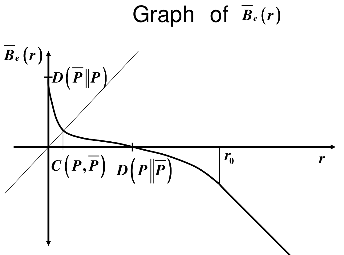
Now, we define the new function B¯​(r)\overline{B}(r):

B¯e​(r):={Be(r|P∥P¯)r≤D(P∥P¯)−Be∗(r|P∥P¯)r>D(P∥P¯).\displaystyle\overline{B}_{e}(r):=\left\{\begin{array}[]{ll}B_{e}(r|P\|\overline{P})&r\leq D(P\|\overline{P})\\ -B_{e}^{*}(r|P\|\overline{P})&r>D(P\|\overline{P}).\end{array}\right.

Then, its graph is shown in Fig. 3.

Refer to caption
Fig. 3: Graph of Be​(r)B_{e}(r)

In order to give other characterizations of (2), we introduce a one-parameter family

Ps,P,P¯​(d​y):=1Φ(s|P∥P)​(∂P¯∂P​(y))s​P​(d​y),\displaystyle P_{s,P,\overline{P}}(dy):=\frac{1}{\Phi(s|P\|P)}(\frac{\partial\overline{P}}{\partial P}(y))^{s}P(dy),

which is abbreviated as PsP_{s}. Then, since ϕ⁡(s)\phi(s) is C1C^{1} continuous,

D(Ps∥P1)\displaystyle D(P_{s}\|P_{1}) =(s−1)ϕ′(s)−ϕ(s)s∈(−∞,1]\displaystyle=(s-1)\phi^{\prime}(s)-\phi(s)\quad s\in(-\infty,1] (4)
D(P0∥Ps)\displaystyle D(P_{0}\|P_{s}) =ϕ⁡(s)−s​ϕ′​(0)s∈[0,∞).\displaystyle=\phi(s)-s\phi^{\prime}(0)\quad s\in[0,\infty). (5)

Since

d⁡(s−1)​ϕ′​(s)−ϕ⁡(s)d​s=−ϕ′′​(s)<0,\displaystyle\frac{d(s-1)\phi^{\prime}(s)-\phi(s)}{ds}=-\phi^{\prime\prime}(s)<0,

D(Ps∥P1)D(P_{s}\|P_{1}) is monotonically decreasing with respect to ss.

As is mentioned in Theorem 4 of Blahut [2], when r≤D(P∥P¯)r\leq D(P\|\overline{P}), there exists sr∈[0,1]s_{r}\in[0,1] such that

minQ:D(Q∥P¯)≤rD(Q∥P)=D(Psr∥P0).\displaystyle\min_{Q:D(Q\|\overline{P})\leq r}D(Q\|P)=D(P_{s_{r}}\|P_{0}).

Then, (4) and (5) imply that

r=D(Psr∥P1)=(sr−1)ϕ(sr)−ϕ(sr).\displaystyle r=D(P_{s_{r}}\|P_{1})=(s_{r}-1)\phi(s_{r})-\phi(s_{r}).

Thus, we obtain another expression.

minQ:D(Q∥P¯)≤rD(Q∥P)=mins∈[0,1]:D(Ps∥P¯)≤rD(Ps∥P).\displaystyle\min_{Q:D(Q\|\overline{P})\leq r}D(Q\|P)=\min_{s\in[0,1]:D(P_{s}\|\overline{P})\leq r}D(P_{s}\|P). (6)

On the other hand,

dd​s​−sr−ϕ(s|P∥P¯)1−s=−r+(s−1)​ϕ′​(s)−ϕ⁡(s)(1−s)2=D(Ps∥P1)(1−s)2.\displaystyle\frac{d}{ds}\frac{-sr-\phi(s|P\|\overline{P})}{1-s}=\frac{-r+(s-1)\phi^{\prime}(s)-\phi(s)}{(1-s)^{2}}=\frac{D(P_{s}\|P_{1})}{(1-s)^{2}}. (7)

Since D(Ps∥P1)D(P_{s}\|P_{1}) is monotonically decreasing with respect to ss, dd​s​−sr−ϕ(s|P∥P¯)1−s=0\frac{d}{ds}\frac{-sr-\phi(s|P\|\overline{P})}{1-s}=0 if and only if s=srs=s_{r}. The equation

minQ:D(Q∥P¯)≤rD(Q∥P)=sup0≤s≤1−sr−ϕ(s|P∥P¯)1−s\displaystyle\min_{Q:D(Q\|\overline{P})\leq r}D(Q\|P)=\sup_{0\leq s\leq 1}\frac{-sr-\phi(s|P\|\overline{P})}{1-s} (8)

can be checked.

In the following, we present some explanations concerning (3). As is mentioned by Han-Kobayashi[10] and Ogawa-Nagaoka[18], when r0:=D(P−∞∥P1)≥r≥D(P∥P¯)r_{0}:=D(P_{-\infty}\|P_{1})\geq r\geq D(P\|\overline{P}), the relation

Be∗(r|P∥P¯)=D(Psr∥P0)\displaystyle B_{e}^{*}(r|P\|\overline{P})=D(P_{s_{r}}\|P_{0})

holds, where sr∈(−∞,0]s_{r}\in(-\infty,0] is defined as

r=D(Psr∥P1)=(sr−1)ϕ(sr)−ϕ(sr).\displaystyle r=D(P_{s_{r}}\|P_{1})=(s_{r}-1)\phi(s_{r})-\phi(s_{r}).

Thus, similar to (6) and (8), the relation

minQ:D(Q∥P¯)≤rD(Q∥P)+r−D(Q∥P¯)\displaystyle\min_{Q:D(Q\|\overline{P})\leq r}D(Q\|P)+r-D(Q\|\overline{P}) =D(Psr∥P)=sups≤0−sr−ϕ(s|P∥P¯)1−s\displaystyle=D(P_{s_{r}}\|P)=\sup_{s\leq 0}\frac{-sr-\phi(s|P\|\overline{P})}{1-s} (9)

holds, where sr≤0s_{r}\leq 0 is defined by D(Psr∥P¯)=rD(P_{s_{r}}\|\overline{P})=r[18].

As mentioned by Nakagawa-Kanaya[22], when r≥r0r\geq r_{0}, the relation

minQ:D(Q∥P¯)≤rD(Q∥P)+r−D(Q∥P¯)=D(P−∞∥P)+r−D(P−∞∥P¯)=minQ:D(Q∥P¯)≤r0(D(Q∥P)+r0−D(Q∥P¯))+r−r0\displaystyle\min_{Q:D(Q\|\overline{P})\leq r}D(Q\|P)+r-D(Q\|\overline{P})=D(P_{-\infty}\|P)+r-D(P_{-\infty}\|\overline{P})=\min_{Q:D(Q\|\overline{P})\leq r_{0}}(D(Q\|P)+r_{0}-D(Q\|\overline{P}))+r-r_{0}

holds. This bound is attained by the following randomized test. The hypothesis PP is accepted with the probability only when the logarithmic likelihood ratio takes the maximum value r0r_{0}. Since D(Ps∥P1)<rD(P_{s}\|P_{1})<r, (7) implies that

sups≤0−sr−ϕ(s|P∥P¯)1−s=lims≤−∞−sr−ϕ(s|P∥P¯)1−s=lims≤−∞−sr0−ϕ(s|P∥P¯)1−s+r−r0\displaystyle\sup_{s\leq 0}\frac{-sr-\phi(s|P\|\overline{P})}{1-s}=\lim_{s\leq-\infty}\frac{-sr-\phi(s|P\|\overline{P})}{1-s}=\lim_{s\leq-\infty}\frac{-sr_{0}-\phi(s|P\|\overline{P})}{1-s}+r-r_{0}
=\displaystyle= minQ:D(Q∥P¯)≤r0(D(Q∥P)+r0−D(Q∥P¯))+r−r0.\displaystyle\min_{Q:D(Q\|\overline{P})\leq r_{0}}(D(Q\|P)+r_{0}-D(Q\|\overline{P}))+r-r_{0}. (10)
Remark 1

The classical Hoeffding bound in information theory is due to Blahut[2] and Csiszár-Longo[4]. The corresponding ideas in statistics were first put forward by Hoeffding[16], from whom the bound received its name. Some authors prefer to refer this bound as the Hoeffding-Blahut-Csiszár- Longo bound.

On the other hand, Han-Kobayashi[10] gave the first equation of (3), and proved that this equation among non-randomized tests when r0≥r≥D(P∥P¯)r_{0}\geq r\geq D(P\|\overline{P}). They pointed out that the minimum minQ:D(Q∥P¯)≤rD(Q∥P)+r−D(Q∥P¯)\min_{Q:D(Q\|\overline{P})\leq r}D(Q\|P)+r-D(Q\|\overline{P}) can be attained by QQ satisfying D(Q∥P¯)=rD(Q\|\overline{P})=r. Ogawa-Nagaoka[18]showed the second equation of (3) for this case.

Nakagawa-Kanaya[22] proved the first equation when r>r0r>r_{0}. Indeed, as pointed by Nakagawa-Kanaya[22], when r>r0r>r_{0}, any non-randomized test cannot attain the minimum minQ:D(Q∥P¯)≤rD(Q∥P)+r−D(Q∥P¯)\min_{Q:D(Q\|\overline{P})\leq r}D(Q\|P)+r-D(Q\|\overline{P}). In this case, the minimum minQ:D(Q∥P¯)≤rD(Q∥P)+r−D(Q∥P¯)\min_{Q:D(Q\|\overline{P})\leq r}D(Q\|P)+r-D(Q\|\overline{P}) cannot be attained by QQ satisfying D(Q∥P¯)=rD(Q\|\overline{P})=r.

III Main result: Adaptive method

Let us focus on two spaces, the set of input signals 𝒳{\cal X} and the set of outputs 𝒴{\cal Y}. In this case, the channel from 𝒳{\cal X} and 𝒴{\cal Y} is described by the map from the set 𝒳{\cal X} to the set of probability distributions on 𝒴{\cal Y}. That is, given a channel WW WxW_{x} represents the output distribution when the input is x∈𝒳x\in{\cal X}. When 𝒳{\cal X} and 𝒴{\cal Y} have finite elements, the channel is given by transition matrix. The main topic is the discrimination of two classical channels WW and W¯\overline{W}. In particular, we treat its asymptotic analysis when we can use the unknown channel only nn times. That is, we discriminate two hypotheses, the null hypothesis H0H_{0} : WnW^{n} versus the alternative hypothesis H1H_{1}: W¯n{\overline{W}}^{n}, where WnW^{n} and W¯n{\overline{W}}^{n} are the nn uses of the channel WW and W¯\overline{W} Then, our problem is to decide which hypothesis is true based on nn inputs x1,…,xnx_{1},\ldots,x_{n} and nn outputs y1,…,yny_{1},\ldots,y_{n}. In this setting, it is allowed to choose the kk-th input based on the previous k−1k-1 output adaptively. We choose the kk-th input xkx_{k} subject to the distribution P(x1,y1),…,(xk−1,yk−1)k​(xk)P^{k}_{(x_{1},y_{1}),\ldots,(x_{k-1},y_{k-1})}(x_{k}) on 𝒳{\cal X}. That is, the kk-th input xkx_{k} depends on kk conditional distributions P→k=(P1,P2,…,Pk)\vec{P}^{k}=(P^{1},P^{2},\ldots,P^{k}). Hence, our decision method is described by nn conditional distributions P→n=(P1,P2,…,Pn)\vec{P}^{n}=(P^{1},P^{2},\ldots,P^{n}) and a [0,1][0,1]-valued function fnf_{n} on (𝒳×𝒴)n({\cal X}\times{\cal Y})^{n}. In this case, when we choose nn inputs x1,…,xnx_{1},\ldots,x_{n} and observe nn outputs y1,…,yny_{1},\ldots,y_{n}, we accept the alternative hypothesis W¯\overline{W} with the probability fn​(x1,y1,…,xn,yn)f_{n}(x_{1},y_{1},\ldots,x_{n},y_{n}). That is, our scheme is illustrated by Fig. 4.

Refer to caption
Fig. 4: The adaptive method

In order to treat this problem mathematically, we introduce the following notation. For a channel WW from 𝒳{\cal X} to 𝒴{\cal Y} and a distribution PP on 𝒳{\cal X}, we define two notations, the distribution W​PWP on 𝒳×𝒴{\cal X}\times{\cal Y} and the distribution W⋅PW\cdot P on 𝒴{\cal Y} as

W​P​(x,y)\displaystyle WP(x,y) :=Wx​(y)​P​(x)\displaystyle:=W_{x}(y)P(x)
W⋅P⁡(x,y)\displaystyle W\cdot P(x,y) :=∫𝒳Wx​(y)​P​(𝑑x).\displaystyle:=\int_{{\cal X}}W_{x}(y)P(dx).

Using the distribution W​PWP, we define two quantities:

D(W∥W¯|P)\displaystyle D(W\|\overline{W}|P) :=D(WP∥W¯P)\displaystyle:=D(WP\|\overline{W}P)
ϕ(s|W∥W¯|P)\displaystyle\phi(s|W\|\overline{W}|P) :=ϕ(s|WP∥W¯P).\displaystyle:=\phi(s|WP\|\overline{W}P).

Based on kk conditional distributions P→k=(P1,P2,…,Pk)\vec{P}^{k}=(P^{1},P^{2},\ldots,P^{k}), we define the following distributions:

QW,P→n\displaystyle Q_{W,\vec{P}^{n}} :=WPnWPn−1⋯WP1\displaystyle:=WP^{n}WP^{n-1}\cdots WP^{1}
PW,P→n\displaystyle P_{W,\vec{P}^{n}} :=Pn⋅QW,P→n−1\displaystyle:=P^{n}\cdot Q_{W,\vec{P}^{n-1}}
Qs,W|W¯,P→n\displaystyle Q_{s,W|\overline{W},\vec{P}^{n}} :=Ps,QW,P→n,QW¯,P→n\displaystyle:=P_{s,Q_{W,\vec{P}^{n}},Q_{\overline{W},\vec{P}^{n}}}
Ps,W|W¯,P→n\displaystyle P_{s,W|\overline{W},\vec{P}^{n}} :=Pn⋅Qs,W|W¯,P→n−1.\displaystyle:=P^{n}\cdot Q_{s,W|\overline{W},\vec{P}^{n-1}}.

Then, the first type of error probability is given by EQW,P→n​fn{\rm E}_{Q_{W,\vec{P}^{n}}}f_{n}, and the second type of error probability is by EQW¯,P→n​(1−fn){\rm E}_{Q_{\overline{W},\vec{P}^{n}}}(1-f_{n}). In order to treat this problem, we introduce the following quantities:

C⁡(W,W¯)\displaystyle C(W,\overline{W}) :=limn→∞−1n​log⁡(minP→n,fn⁡EQW,P→n​fn+EQW¯,P→n​(1−fn))\displaystyle:=\lim_{n\rightarrow\infty}\frac{-1}{n}\log(\min_{\vec{P}^{n},f_{n}}{\rm E}_{Q_{W,\vec{P}^{n}}}f_{n}+{\rm E}_{Q_{\overline{W},\vec{P}^{n}}}(1-f_{n}))
βn∗​(ϵ)\displaystyle\beta_{n}^{*}(\epsilon) :=minP→n,fn⁡{EQW¯,P→n​(1−fn)|EQW,P→n​fn≤ϵ},\displaystyle:=\min_{\vec{P}^{n},f_{n}}\bigl\{{\rm E}_{Q_{\overline{W},\vec{P}^{n}}}(1-f_{n})\bigm|{\rm E}_{Q_{W,\vec{P}^{n}}}f_{n}\leq\epsilon\bigr\},

and

B(W∥W¯):=\displaystyle B(W\|\overline{W}):= sup{(P→n,fn)}{lim¯n→∞−log⁡EQW¯,P→n​(1−fn)n|limn→∞EQW,P→nfn=0}\displaystyle\sup_{\{(\vec{P}^{n},f_{n})\}}\left\{\left.\varliminf_{n\rightarrow\infty}\frac{-\log{\rm E}_{Q_{\overline{W},\vec{P}^{n}}}(1-f_{n})}{n}\right|\lim_{n\rightarrow\infty}{\rm E}_{Q_{W,\vec{P}^{n}}}f_{n}=0\right\}
B∗(W∥W¯):=\displaystyle B^{*}(W\|\overline{W}):= inf{(P→n,fn)}{lim¯n→∞−log⁡EQW¯,P→n​(1−fn)n|lim¯n→∞EQW,P→nfn<1}\displaystyle\inf_{\{(\vec{P}^{n},f_{n})\}}\left\{\left.\varliminf_{n\rightarrow\infty}\frac{-\log{\rm E}_{Q_{\overline{W},\vec{P}^{n}}}(1-f_{n})}{n}\right|\varliminf_{n\rightarrow\infty}{\rm E}_{Q_{W,\vec{P}^{n}}}f_{n}<1\right\}
Be(r|W∥W¯):=\displaystyle B_{e}(r|W\|\overline{W}):= sup{(P→n,fn)}{lim¯n→∞−log⁡EQW,P→n​fnn|lim¯n→∞−log⁡EQW¯,P→n​(1−fn)n≥r}\displaystyle\sup_{\{(\vec{P}^{n},f_{n})\}}\left\{\left.\varliminf_{n\rightarrow\infty}\frac{-\log{\rm E}_{Q_{W,\vec{P}^{n}}}f_{n}}{n}\right|\varliminf_{n\rightarrow\infty}\frac{-\log{\rm E}_{Q_{\overline{W},\vec{P}^{n}}}(1-f_{n})}{n}\geq r\right\}
Be∗(r|W∥W¯):=\displaystyle B_{e}^{*}(r|W\|\overline{W}):= inf{(P→n,fn)}{lim¯n→∞−log⁡EQW,P→n​(1−fn)n|lim¯n→∞−log⁡EQW¯,P→n​(1−fn)n≥r}.\displaystyle\inf_{\{(\vec{P}^{n},f_{n})\}}\left\{\left.\varliminf_{n\rightarrow\infty}\frac{-\log{\rm E}_{Q_{W,\vec{P}^{n}}}(1-f_{n})}{n}\right|\varliminf_{n\rightarrow\infty}\frac{-\log{\rm E}_{Q_{\overline{W},\vec{P}^{n}}}(1-f_{n})}{n}\geq r\right\}.

We obtain the following channel version of Stein’s lemma.

Theorem 1

Assume that ϕ(s|Wx∥W¯x)\phi(s|W_{x}\|\overline{W}_{x}) is C1C^{1} continuous, and

limϵ→+0ϕ(−ϵ|W∥W¯)ϵ=supx∈𝒳D(Wx∥W¯x),\displaystyle\lim_{\epsilon\to+0}\frac{\phi(-\epsilon|W\|\overline{W})}{\epsilon}=\sup_{x\in{\cal X}}D(W_{x}\|\overline{W}_{x}), (11)

where ϕ(s|W∥W¯):=supx∈𝒳ϕ(s|Wx|W¯x)=supP∈𝒫⁡(𝒳)ϕ(s|W∥W¯|P)\phi(s|W\|\overline{W}):=\sup_{x\in{\cal X}}\phi(s|W_{x}|\overline{W}_{x})=\sup_{P\in{\cal P}({\cal X})}\phi(s|W\|\overline{W}|P), and 𝒫⁡(𝒳){\cal P}({\cal X}) is the set of distributions on 𝒳{\cal X}.

Then,

B(W∥W¯)=B∗(W∥W¯)=D¯:=supx∈𝒳D(Wx∥W¯x).\displaystyle B(W\|\overline{W})=B^{*}(W\|\overline{W})=\overline{D}:=\sup_{x\in{\cal X}}D(W_{x}\|\overline{W}_{x}). (12)

The following is another expression of Stein’s lemma.

Corollary 1

Under the same assumption,

limn→∞−1n​log⁡βn∗​(ϵ)\displaystyle\lim_{n\rightarrow\infty}\frac{-1}{n}\log\beta_{n}^{*}(\epsilon) =supx∈𝒳D(Wx∥W¯x).\displaystyle=\sup_{x\in{\cal X}}D(W_{x}\|\overline{W}_{x}).

Condition (11) can be replaced by another condition.

Lemma 1

When any element x∈𝒳x\in{\cal X} satisfies

ϕ′(0|Wx∥W¯x)=D(Wx∥W¯x)\displaystyle\phi^{\prime}(0|W_{x}\|\overline{W}_{x})=D(W_{x}\|\overline{W}_{x})

and there exists a real number ϵ>0\epsilon>0 such that

C1:=supx∈𝒳sups∈[−ϵ,0]d2ϕ(s|Wx∥W¯x)d​s2\displaystyle C_{1}:=\sup_{x\in{\cal X}}\sup_{s\in[-\epsilon,0]}\frac{d^{2}\phi(s|W_{x}\|\overline{W}_{x})}{ds^{2}} <∞,\displaystyle<\infty, (13)

then condition (11) holds.

In addition, we obtain a channel version of the Hoeffding bound.

Theorem 2

When

supx∈𝒳sups∈[0,1]d2ϕ(s|Wx∥W¯x)d​s2\displaystyle\sup_{x\in{\cal X}}\sup_{s\in[0,1]}\frac{d^{2}\phi(s|W_{x}\|\overline{W}_{x})}{ds^{2}} <∞\displaystyle<\infty (14)

and

supx∈𝒳D(W¯x∥Wx)<∞,\displaystyle\sup_{x\in{\cal X}}D(\overline{W}_{x}\|W_{x})<\infty,

then

Be(r|W∥W¯)\displaystyle B_{e}(r|W\|\overline{W}) =supx∈𝒳sup0≤s≤1−sr−ϕ(s|Wx∥W¯x)1−s=supx∈𝒳minQ:D(Q∥W¯x)≤rD(Q∥Wx).\displaystyle=\sup_{x\in{\cal X}}\sup_{0\leq s\leq 1}\frac{-sr-\phi(s|W_{x}\|\overline{W}_{x})}{1-s}=\sup_{x\in{\cal X}}\min_{Q:D(Q\|\overline{W}_{x})\leq r}D(Q\|W_{x}). (15)
Corollary 2

Under the same assumption,

C⁡(W,W¯)\displaystyle C(W,\overline{W}) =supx∈𝒳−min0≤s≤1ϕ(s|Wx∥W¯x).\displaystyle=\sup_{x\in{\cal X}}-\min_{0\leq s\leq 1}\phi(s|W_{x}\|\overline{W}_{x}). (16)

These arguments imply that adaptive improvement does not improve the performance in the above senses. For example, when we apply the best input xM:=argmaxxD(Wx∥W¯x)x_{M}:=\mathop{\rm argmax}_{x}D(W_{x}\|\overline{W}_{x}) to all of nn channels, we can achieve the optimal performance in the sense of the Stein bound. The same fact is true concerning the Hoeffding bound and the Chernoff bound.

Proof:

The relation

C(W,W¯)=sup{r|Be(r|W∥W¯)≥r}\displaystyle C(W,\overline{W})=\sup\{r|B_{e}(r|W\|\overline{W})\geq r\}

holds. Since

sup{r|supx∈𝒳sup0≤s≤1−sr−ϕ(s|Wx∥W¯x)1−s≥r}\displaystyle\sup\Bigl\{r\Bigl|\sup_{x\in{\cal X}}\sup_{0\leq s\leq 1}\frac{-sr-\phi(s|W_{x}\|\overline{W}_{x})}{1-s}\geq r\Bigr.\Bigr\}
=\displaystyle= supx∈𝒳sup{r|sup0≤s≤1−sr−ϕ(s|Wx∥W¯x)1−s≥r}\displaystyle\sup_{x\in{\cal X}}\sup\Bigl\{r\Bigl|\sup_{0\leq s\leq 1}\frac{-sr-\phi(s|W_{x}\|\overline{W}_{x})}{1-s}\geq r\Bigr.\Bigr\}
=\displaystyle= supx∈𝒳−min0≤s≤1ϕ(s|Wx∥W¯x),\displaystyle\sup_{x\in{\cal X}}-\min_{0\leq s\leq 1}\phi(s|W_{x}\|\overline{W}_{x}),

the relation (16) holds. ∎

The channel version of the Han-Kobayashi bound is given as follows.

Theorem 3

When ϕ(s|Wx∥W¯x)\phi(s|W_{x}\|\overline{W}_{x}) is C1C^{1} continuous, then

Be∗(r|W∥W¯)\displaystyle B_{e}^{*}(r|W\|\overline{W}) =sups≤0−sr−ϕ(s|W∥W¯)1−s=infP∈𝒫⁡(𝒳)sups≤0−sr−ϕ(s|W∥W¯|P)1−s=infP∈𝒫2​(𝒳)sups≤0−sr−ϕ(s|W∥W¯|P)1−s,\displaystyle=\sup_{s\leq 0}\frac{-sr-\phi(s|W\|\overline{W})}{1-s}=\inf_{P\in{\cal P}({\cal X})}\sup_{s\leq 0}\frac{-sr-\phi(s|W\|\overline{W}|P)}{1-s}=\inf_{P\in{\cal P}^{2}({\cal X})}\sup_{s\leq 0}\frac{-sr-\phi(s|W\|\overline{W}|P)}{1-s}, (17)

where 𝒫2​(𝒳){\cal P}^{2}({\cal X}) is the distribution on 𝒳{\cal X} that takes positive probability only on at most two elements.

As shown in Section IV, the equality

sups≤0−sr−ϕ(s|W∥W¯)1−s=infx∈𝒳sups≤0−sr−ϕ(s|Wx∥W¯x)1−s\displaystyle\sup_{s\leq 0}\frac{-sr-\phi(s|W\|\overline{W})}{1-s}=\inf_{x\in{\cal X}}\sup_{s\leq 0}\frac{-sr-\phi(s|W_{x}\|\overline{W}_{x})}{1-s} (18)

does not necessarily hold in general. In order to understand the meaning of this fact, we assume that the equation (18) does not hold. When we apply the same input xx to all channels, the best performance cannot be achieved. However, the best performance can be achieved by the following method. Assume that the best input distribution argmaxP∈𝒫2​(𝒳)sups≤0−sr−ϕ(s|W∥W¯|P)1−s\mathop{\rm argmax}_{P\in{\cal P}^{2}({\cal X})}\sup_{s\leq 0}\frac{-sr-\phi(s|W\|\overline{W}|P)}{1-s} has the support {x,x′}\{x,x^{\prime}\}, and the probabilities λ\lambda and 1−λ1-\lambda. Then, applying xx or x′x^{\prime} to all channels with the probability λ\lambda and 1−λ1-\lambda, we can achieve the best performance in the sense of the Han-Kobayashi bound. That is, the structure of optimal strategy of the Han-Kobayashi bound is more complex than those of the above cases.

IV Simple example

In this section, we treat a simple example that does not satisfy (18). For four given parameters p,q,a>1,b>1p,q,a>1,b>1, we define the channels WW and W¯\overline{W}:

W0​(0):=a​q,W0​(1):=1−a​q,\displaystyle W_{0}(0):=aq,\quad W_{0}(1):=1-aq,
W¯0​(0):=q,W¯0​(1):=1−q,\displaystyle\overline{W}_{0}(0):=q,\quad\overline{W}_{0}(1):=1-q,
W1​(0):=b​q,W1​(1):=1−b​q,\displaystyle W_{1}(0):=bq,\quad W_{1}(1):=1-bq,
W¯1​(0):=q,W¯1​(1):=1−q.\displaystyle\overline{W}_{1}(0):=q,\quad\overline{W}_{1}(1):=1-q.

Then, we obtain

lims→−∞ϕ(s|W0∥W¯0)s=a,\displaystyle\lim_{s\to-\infty}\frac{\phi(s|W_{0}\|\overline{W}_{0})}{s}=a,
lims→−∞ϕ(s|W1∥W¯1)s=b.\displaystyle\lim_{s\to-\infty}\frac{\phi(s|W_{1}\|\overline{W}_{1})}{s}=b.

In this case,

D(W0∥W¯0)=\displaystyle D(W_{0}\|\overline{W}_{0})= a​p​log⁡a+(1−a​p)​log⁡1−a​p1−p\displaystyle ap\log a+(1-ap)\log\frac{1-ap}{1-p}
D(W1∥W¯1)=\displaystyle D(W_{1}\|\overline{W}_{1})= b​q​log⁡b+(1−b​q)​log⁡1−b​q1−q.\displaystyle bq\log b+(1-bq)\log\frac{1-bq}{1-q}.

When a>ba>b and D(W0∥W¯0)<D(W1∥W¯1)D(W_{0}\|\overline{W}_{0})<D(W_{1}\|\overline{W}_{1}), the magnitude relation between ϕ(s|W0∥W¯0)\phi(s|W_{0}\|\overline{W}_{0}) and ϕ(s|W1∥W¯1)\phi(s|W_{1}\|\overline{W}_{1}) on (−∞,0)(-\infty,0) depends on s∈(−∞,0)s\in(-\infty,0). For example, the case of a=100,b=1.5,p=0.0001,q=0.65a=100,b=1.5,p=0.0001,q=0.65 is shown in Fig. 5. In this case, Be∗(r|W0∥W¯0)B_{e}^{*}(r|W_{0}\|\overline{W}_{0}), Be∗(r|W1∥W¯1)B_{e}^{*}(r|W_{1}\|\overline{W}_{1}), and Be∗(r|W∥W¯)B_{e}^{*}(r|W\|\overline{W}) are calculated by Fig. 6. Then, the inequality (18) does not hold.

Refer to caption
Fig. 5: Magnitude relation between ϕ(s|W0∥W¯0)\phi(s|W_{0}\|\overline{W}_{0}) and ϕ(s|W1∥W¯1)\phi(s|W_{1}\|\overline{W}_{1}) on (−1,0)(-1,0). The upper solid line indicates ϕ(s|W0∥W¯0)\phi(s|W_{0}\|\overline{W}_{0}), the dotted line indicates ϕ(s|W1∥W¯1)\phi(s|W_{1}\|\overline{W}_{1}).
Refer to caption
Fig. 6: Magnitude relation between Be∗(r|W0∥W¯0)B_{e}^{*}(r|W_{0}\|\overline{W}_{0}), Be∗(r|W1∥W¯1)B_{e}^{*}(r|W_{1}\|\overline{W}_{1}), and Be∗(r|W∥W¯)B_{e}^{*}(r|W\|\overline{W}) on (−1,0)(-1,0). The upper solid line indicates Be∗(r|W0∥W¯0)B_{e}^{*}(r|W_{0}\|\overline{W}_{0}), the dotted line indicates Be∗(r|W1∥W¯1)B_{e}^{*}(r|W_{1}\|\overline{W}_{1}), and the lower solid line indicates Be∗(r|W∥W¯)B_{e}^{*}(r|W\|\overline{W}).

V Application to adaptive quantum state discrimination

Quantum state discrimination between two states ρ\rho and σ\sigma on a dd-dimensional system ℋ{\cal H} with nn copies by one-way LOCC is formulated as follows. We choose the first POVM M1M_{1} and obtain the data y1y_{1} through the measurement M1M_{1}. In the kk-th step, we choose the kk-th POVM Mk​((M1,y1),…,(Mk−1,yk−1))M_{k}((M_{1},y_{1}),\ldots,(M_{k-1},y_{k-1})) depending on (M1,y1),…,(Mk−1,yk−1)(M_{1},y_{1}),\ldots,(M_{k-1},y_{k-1}). Then, we obtain the kk-th data yky_{k} through Mk​((M1,y1),…,(Mk−1,yk−1))M_{k}((M_{1},y_{1}),\ldots,(M_{k-1},y_{k-1})). Therefore, this problem can be regarded as classical channel discrimination with the correspondence WM​(y)=TrM⁡(y)​ρW_{M}(y)=\mathop{\rm Tr}\nolimits M(y)\rho and W¯M​(y)=TrM⁡(y)​σ\overline{W}_{M}(y)=\mathop{\rm Tr}\nolimits M(y)\sigma. That is, in this case, the set of input signal corresponds to the set of extremal points of the set of POVMs on the given system ℋ{\cal H}. The proposed scheme is illustrated in Fig. 7.

Refer to caption
Fig. 7: Adaptive quantum state discrimination

Now, we assume that ρ>0\rho>0 and σ>0\sigma>0. In this case, 𝒳{\cal X} is compact, and the map (s,M)→d2ϕ(s|WM∥W¯M)d​s2(s,M)\to\frac{d^{2}\phi(s|W_{M}\|\overline{W}_{M})}{ds^{2}} is continuous. Then, the condition (13) holds. Therefore, one-way improvement does not improve the performance in the sense of the Stein bound, the Chernoff bound, the Hoeffding bound, or the Han-Kobayashi bound. That is, we obtain

B(W∥W¯)=\displaystyle B(W\|\overline{W})= B∗(W∥W¯)=maxM:POVMD(PρM∥PσM)\displaystyle B^{*}(W\|\overline{W})=\max_{M:{\rm POVM}}D(P^{M}_{\rho}\|P^{M}_{\sigma})
Be(r|W∥W¯)=\displaystyle B_{e}(r|W\|\overline{W})= maxM:POVMsup0≤s≤1−sr−ϕ(s|PMρ∥PMσ)1−s\displaystyle\max_{M:{\rm POVM}}\sup_{0\leq s\leq 1}\frac{-sr-\phi(s|P^{M}_{\rho}\|P^{M}_{\sigma})}{1-s}
Be∗(r|W∥W¯)=\displaystyle B_{e}^{*}(r|W\|\overline{W})= sups≤0−sr−maxM:POVMϕ(s|PMρ∥PMσ)1−s.\displaystyle\sup_{s\leq 0}\frac{-sr-\max_{M:{\rm POVM}}\phi(s|P^{M}_{\rho}\|P^{M}_{\sigma})}{1-s}.

Therefore, there exists a difference between one-way LOCC and collective measurement.

VI Proof of the Stein bound: (12)

Now, we prove the Stein bound: (12). For any x∈𝒳x\in{\cal X}, by choosing the input xx in nn times, we obtain

B(W∥W¯)≥D(Wx∥W¯x).\displaystyle B(W\|\overline{W})\geq D(W_{x}\|\overline{W}_{x}).

Taking the supremum, we have

B(W∥W¯)≥supx∈𝒳D(Wx∥W¯x).\displaystyle B(W\|\overline{W})\geq\sup_{x\in{\cal X}}D(W_{x}\|\overline{W}_{x}).

Furthermore, from the definition, it is trivial that

B(W∥W¯)≤B∗(W∥W¯).\displaystyle B(W\|\overline{W})\leq B^{*}(W\|\overline{W}).

Therefore, it is sufficient to show the strong converse part:

B∗(W∥W¯)≤D¯.\displaystyle B^{*}(W\|\overline{W})\leq\overline{D}. (19)

However, in preparation for the proof of (15), we present a proof of the weak converse part:

B(W∥W¯)≤D¯\displaystyle B(W\|\overline{W})\leq\overline{D} (20)

which is weaker argument than (19), and is valid without assumption (11). In the following proof, it is essential to evaluate the KL-divergence concerning the obtained data.

In order to prove (20), we prove that

lim¯n→∞−1nlogEQW¯,P→n(1−fn)≤D¯\displaystyle\varlimsup_{n\to\infty}-\frac{1}{n}\log{\rm E}_{Q_{\overline{W},\vec{P}^{n}}}(1-f_{n})\leq\overline{D} (21)

when

EQW,P→n​fn→0.\displaystyle{\rm E}_{Q_{W,\vec{P}^{n}}}f_{n}\to 0. (22)

It follows from the definitions of QW,P→nQ_{W,\vec{P}^{n}} and QW¯,P→nQ_{\overline{W},\vec{P}^{n}} that

D(QW,P→n∥QW¯,P→n)=∑k=1nD(W∥W¯|PW,P→k).\displaystyle D(Q_{W,\vec{P}^{n}}\|Q_{\overline{W},\vec{P}^{n}})=\sum_{k=1}^{n}D(W\|\overline{W}|P_{W,\vec{P}^{k}}).

Since −EQW,P→n​fn​log⁡EQW¯,P→n​fn≥0-{\rm E}_{Q_{W,\vec{P}^{n}}}f_{n}\log{\rm E}_{Q_{\overline{W},\vec{P}^{n}}}f_{n}\geq 0, information processing inequality concerning the KL divergence yields the following:

−h⁡(EQW,P→n​(1−fn))−(EQW,P→n​(1−fn))​log⁡EQW¯,P→n​(1−fn)\displaystyle-h({\rm E}_{Q_{W,\vec{P}^{n}}}(1-f_{n}))-({\rm E}_{Q_{W,\vec{P}^{n}}}(1-f_{n}))\log{\rm E}_{Q_{\overline{W},\vec{P}^{n}}}(1-f_{n})
≤\displaystyle\leq EQW,P→n​(1−fn)​(log⁡EQW,P→n​(1−fn)−log⁡EQW¯,P→n​(1−fn))+EQW,P→n​fn​(log⁡EQW,P→n​fn−log⁡EQW¯,P→n​fn)\displaystyle{\rm E}_{Q_{W,\vec{P}^{n}}}(1-f_{n})(\log{\rm E}_{Q_{W,\vec{P}^{n}}}(1-f_{n})-\log{\rm E}_{Q_{\overline{W},\vec{P}^{n}}}(1-f_{n}))+{\rm E}_{Q_{W,\vec{P}^{n}}}f_{n}(\log{\rm E}_{Q_{W,\vec{P}^{n}}}f_{n}-\log{\rm E}_{Q_{\overline{W},\vec{P}^{n}}}f_{n})
≤\displaystyle\leq D(QW,P→n∥QW¯,P→n)=∑k=1nD(W∥W¯|PW,P→k)≤nD¯.\displaystyle D(Q_{W,\vec{P}^{n}}\|Q_{\overline{W},\vec{P}^{n}})=\sum_{k=1}^{n}D(W\|\overline{W}|P_{W,\vec{P}^{k}})\leq n\overline{D}. (23)

That is,

−1n​log⁡EQW¯,P→n​(1−fn)≤D¯+1n​h​(EQW,P→n​(1−fn))EQW,P→n​(1−fn).\displaystyle-\frac{1}{n}\log{\rm E}_{Q_{\overline{W},\vec{P}^{n}}}(1-f_{n})\leq\frac{\overline{D}+\frac{1}{n}h({\rm E}_{Q_{W,\vec{P}^{n}}}(1-f_{n}))}{{\rm E}_{Q_{W,\vec{P}^{n}}}(1-f_{n})}. (24)

Therefore, (22) yields (21).

Next, we prove the strong converse part, i.e., we show that

EQW,P→n​(1−fn)→0\displaystyle{\rm E}_{Q_{W,\vec{P}^{n}}}(1-f_{n})\to 0 (25)

when

r:=lim¯n→∞⁡−log⁡EQW¯,P→n​(1−fn)n>D¯.\displaystyle r:=\varliminf_{n\rightarrow\infty}\frac{-\log{\rm E}_{Q_{\overline{W},\vec{P}^{n}}}(1-f_{n})}{n}>\overline{D}. (26)

Since

Φ(s|QW,P→n∥QW¯,P→n)\displaystyle\Phi(s|Q_{W,\vec{P}^{n}}\|Q_{\overline{W},\vec{P}^{n}})
=\displaystyle= Φ(s|QW,P→n−1∥QW¯,P→n−1)(∫𝒳(∫𝒴(∂Wxn′∂Wxn(yn))sWxn(dyn))Ps,W|W¯,P→n(dxn)),\displaystyle\Phi(s|Q_{W,\vec{P}^{n-1}}\|Q_{\overline{W},\vec{P}^{n-1}})\left(\int_{{\cal X}}\left(\int_{{\cal Y}}(\frac{\partial W_{x_{n}}^{\prime}}{\partial W_{x_{n}}}(y_{n}))^{s}W_{x_{n}}(dy_{n})\right)P_{s,W|\overline{W},\vec{P}^{n}}(dx_{n})\right),

we obtain

ϕ(s|QW,P→n∥QW¯,P→n)=ϕ(s|QW,P→n−1∥QW¯,P→n−1)+ϕ(s|W∥W¯|Ps,W|W¯,P→n).\displaystyle\phi(s|Q_{W,\vec{P}^{n}}\|Q_{\overline{W},\vec{P}^{n}})=\phi(s|Q_{W,\vec{P}^{n-1}}\|Q_{\overline{W},\vec{P}^{n-1}})+\phi(s|W\|\overline{W}|P_{s,W|\overline{W},\vec{P}^{n}}). (27)

Applying (27) inductively, we obtain the relation

ϕ(s|QW,P→n∥QW¯,P→n)=∑k=1nϕ(s|W∥W¯|Ps,W|W¯,P→k)≤nϕ(s|W∥W¯).\displaystyle\phi(s|Q_{W,\vec{P}^{n}}\|Q_{\overline{W},\vec{P}^{n}})=\sum_{k=1}^{n}\phi(s|W\|\overline{W}|P_{s,W|\overline{W},\vec{P}^{k}})\leq n\phi(s|W\|\overline{W}). (28)

Since the information quantity ϕ(s|P∥P¯)\phi(s|P\|\overline{P}) satisfies the information processing inequality, we have

(EQW,P→n​(1−fn))1−s​(EQW¯,P→n​(1−fn))s\displaystyle({\rm E}_{Q_{W,\vec{P}^{n}}}(1-f_{n}))^{1-s}({\rm E}_{Q_{\overline{W},\vec{P}^{n}}}(1-f_{n}))^{s}
≤\displaystyle\leq (EQW,P→n​(1−fn))1−s​(EQW¯,P→n​(1−fn))s+(EQW,P→n​fn)1−s​(EQW¯,P→n​fn)s\displaystyle({\rm E}_{Q_{W,\vec{P}^{n}}}(1-f_{n}))^{1-s}({\rm E}_{Q_{\overline{W},\vec{P}^{n}}}(1-f_{n}))^{s}+({\rm E}_{Q_{W,\vec{P}^{n}}}f_{n})^{1-s}({\rm E}_{Q_{\overline{W},\vec{P}^{n}}}f_{n})^{s}
≤\displaystyle\leq eϕ(s|QW,P→n∥QW¯,P→n)\displaystyle e^{\phi(s|Q_{W,\vec{P}^{n}}\|Q_{\overline{W},\vec{P}^{n}})}
≤\displaystyle\leq enϕ(s|W∥W¯),\displaystyle e^{n\phi(s|W\|\overline{W})},

for s≤0s\leq 0. Taking the logarithm, we obtain

(1−s)logEQW,P→n(1−fn)≤−slogEQW¯,P→n(1−fn)+nϕ(s|W∥W¯).\displaystyle(1-s)\log{\rm E}_{Q_{W,\vec{P}^{n}}}(1-f_{n})\leq-s\log{\rm E}_{Q_{\overline{W},\vec{P}^{n}}}(1-f_{n})+n\phi(s|W\|\overline{W}). (29)

That is,

−1n​log⁡EQW,P→n​(1−fn)≥−s−1nlogEQW¯,P→n(1−fn)−ϕ(s|W∥W¯)1−s.\displaystyle\frac{-1}{n}\log{\rm E}_{Q_{W,\vec{P}^{n}}}(1-f_{n})\geq\frac{-s\frac{-1}{n}\log{\rm E}_{Q_{\overline{W},\vec{P}^{n}}}(1-f_{n})-\phi(s|W\|\overline{W})}{1-s}.

When lim¯n→∞⁡−log⁡EP¯n​(1−fn)n≥r\varliminf_{n\rightarrow\infty}\frac{-\log{\rm E}_{{\overline{P}}^{n}}(1-f_{n})}{n}\geq r, the inequality

Be∗(r|W∥W¯)≥lim¯n→∞−1nlogEQW,P→n(1−fn)≥−sr−ϕ(s|W∥W¯)1−s\displaystyle B_{e}^{*}(r|W\|\overline{W})\geq\varliminf_{n\rightarrow\infty}\frac{-1}{n}\log{\rm E}_{Q_{W,\vec{P}^{n}}}(1-f_{n})\geq\frac{-sr-\phi(s|W\|\overline{W})}{1-s}

holds. Taking the supremum, we obtain

Be∗(r|W∥W¯)≥sups≤0−sr−ϕ(s|W∥W¯)1−s.\displaystyle B_{e}^{*}(r|W\|\overline{W})\geq\sup_{s\leq 0}\frac{-sr-\phi(s|W\|\overline{W})}{1-s}.

From conditions (11) and (26), there exists a small real number ϵ>0\epsilon>0 such that r>ϕ(−ϵ|W∥W¯)−ϵr>\frac{\phi(-\epsilon|W\|\overline{W})}{-\epsilon}. Thus,

sups≤0−sr−ϕ(s|W∥W¯)1−s≥ϵr−ϕ(−ϵ|W∥W¯)1+ϵ>0.\displaystyle\sup_{s\leq 0}\frac{-sr-\phi(s|W\|\overline{W})}{1-s}\geq\frac{\epsilon r-\phi(-\epsilon|W\|\overline{W})}{1+\epsilon}>0.

Therefore, we obtain (25).

Remark 2

The technique of the strong converse part except for (28) was developed by Nagaoka [19]. Hence, deriving (28) can be regarded as the main contribution in this section of the present paper.

Proof of Lemma 1:

It is sufficient for a proof of (11) to show that the uniformity of the convergence ϕ(−ϵ|Wx∥W¯x)ϵ−D(Wx∥W¯x)→0\frac{\phi(-\epsilon|W_{x}\|\overline{W}_{x})}{\epsilon}-D(W_{x}\|\overline{W}_{x})\to 0 concerning x∈𝒳x\in{\cal X}. Now, we choose ϵ>0\epsilon>0 satisfying condition (13). Then, there exists s∈[−ϵ,0]s\in[-\epsilon,0] such that ϕ(−ϵ|Wx∥W¯x)ϵ−D(Wx∥W¯x)=12ϵϕ(s|Wx∥W¯x)≤C12ϵ\frac{\phi(-\epsilon|W_{x}\|\overline{W}_{x})}{\epsilon}-D(W_{x}\|\overline{W}_{x})=\frac{1}{2}\epsilon\phi(s|W_{x}\|\overline{W}_{x})\leq\frac{C_{1}}{2}\epsilon. Therefore, the condition (11) holds.

VII Proof of the Hoeffding bound: (15)

In this section, we prove the Hoeffding bound: (15). Since the inequality

Be(r|W∥W¯)≥supx∈𝒳sup0≤s≤1−sr−ϕ(s|Wx∥W¯x)1−s=supx∈𝒳minQ:D(Q∥W¯x)≤rD(Q∥Wx)\displaystyle B_{e}(r|W\|\overline{W})\geq\sup_{x\in{\cal X}}\sup_{0\leq s\leq 1}\frac{-sr-\phi(s|W_{x}\|\overline{W}_{x})}{1-s}=\sup_{x\in{\cal X}}\min_{Q:D(Q\|\overline{W}_{x})\leq r}D(Q\|W_{x})

is trivial, we prove the opposite inequality. In the following proof, the geometric characterization Fig. 1 and the weak and the strong converse parts are essential. Equation (6) guarantees that

supx∈𝒳minQ:D(Q∥W¯x)≤rD(Q∥Wx)=supx∈𝒳mins∈[0,1]:D(Ps,Wx,W¯x∥W¯x)≤rD(Ps,Wx,W¯x∥Wx).\displaystyle\sup_{x\in{\cal X}}\min_{Q:D(Q\|\overline{W}_{x})\leq r}D(Q\|W_{x})=\sup_{x\in{\cal X}}\min_{s\in[0,1]:D(P_{s,W_{x},\overline{W}_{x}}\|\overline{W}_{x})\leq r}D(P_{s,W_{x},\overline{W}_{x}}\|W_{x}).

For this purpose, for arbitrary ϵ>0\epsilon>0, we choose a channel V:Vx=Ps⁡(x),Wx,W¯xV:V_{x}=P_{s(x),W_{x},\overline{W}_{x}} by

s(x):=argmins∈[0,1]:D(Ps,Wx,W¯x∥W¯x)≤rD(Ps,Wx,W¯x∥Wx).\displaystyle s(x):=\mathop{\rm argmin}_{s\in[0,1]:D(P_{s,W_{x},\overline{W}_{x}}\|\overline{W}_{x})\leq r}D(P_{s,W_{x},\overline{W}_{x}}\|W_{x}).

Assume that a sequence {(P→n,fn)}\{(\vec{P}^{n},f_{n})\} satisfies

lim¯n→∞⁡−1n​log⁡EQW¯,P→n​(1−fn)=r.\displaystyle\varlimsup_{n\to\infty}\frac{-1}{n}\log{\rm E}_{Q_{\overline{W},\vec{P}^{n}}}(1-f_{n})=r.

By substituting VV into WW, the strong converse part of the Stein bound:(25) implies that

limEQV,P→n​(1−fn)=0.\displaystyle\lim{\rm E}_{Q_{V,\vec{P}^{n}}}(1-f_{n})=0.

The condition (13) can be checked by the following relations:

dϕ(t|Ps⁡(x),Wx,W¯x∥W¯x)d​t\displaystyle\frac{d\phi(t|P_{s(x),W_{x},\overline{W}_{x}}\|\overline{W}_{x})}{dt} =(1−s(x))ϕ′(s(x)(1−t)+t|Wx∥W¯x)\displaystyle=(1-s(x))\phi^{\prime}(s(x)(1-t)+t|W_{x}\|\overline{W}_{x}) (30)
d2ϕ(t|Ps⁡(x),Wx,W¯x∥W¯x)d​t2\displaystyle\frac{d^{2}\phi(t|P_{s(x),W_{x},\overline{W}_{x}}\|\overline{W}_{x})}{dt^{2}} =(1−s(x))2ϕ′′(s(x)(1−t)+t|Wx∥W¯x).\displaystyle=(1-s(x))^{2}\phi^{\prime\prime}(s(x)(1-t)+t|W_{x}\|\overline{W}_{x}). (31)

Thus, by substituting VV and WW into WW and W¯\overline{W}, the relation (24) implies that

lim¯n→∞−1nlogEQW¯,P→n(1−fn)≤supx∈𝒳D(Vx∥Wx).\displaystyle\varlimsup_{n\to\infty}-\frac{1}{n}\log{\rm E}_{Q_{\overline{W},\vec{P}^{n}}}(1-f_{n})\leq\sup_{x\in{\cal X}}D(V_{x}\|W_{x}).

Similar to (30) and (31), we can check the condition (13).

From the construction of VV, we obtain

lim¯n→∞−1nlogEQW¯,P→n(1−fn)≤maxxminQ:D(Q∥W¯x)≤r−ϵD(Q∥Wx).\displaystyle\varlimsup_{n\to\infty}-\frac{1}{n}\log{\rm E}_{Q_{\overline{W},\vec{P}^{n}}}(1-f_{n})\leq\max_{x}\min_{Q:D(Q\|\overline{W}_{x})\leq r-\epsilon}D(Q\|W_{x}).

The uniform continuity guarantees that

lim¯n→∞−1nlogEQW¯,P→n(1−fn)≤maxxminQ:D(Q∥W¯x)≤rD(Q∥Wx).\displaystyle\varlimsup_{n\to\infty}-\frac{1}{n}\log{\rm E}_{Q_{\overline{W},\vec{P}^{n}}}(1-f_{n})\leq\max_{x}\min_{Q:D(Q\|\overline{W}_{x})\leq r}D(Q\|W_{x}).

Now, we show the uniformity of the function r↦sup0≤s≤1−sr−ϕ(s|Wx∥W¯x)1−sr\mapsto\sup_{0\leq s\leq 1}\frac{-sr-\phi(s|W_{x}\|\overline{W}_{x})}{1-s} concerning xx. As mentioned in p. 82 of Hayashi[11], the relation

dd​r​sup0≤s≤1−sr−ϕ(s|Wx∥W¯x)1−s=srsr−1\displaystyle\frac{d}{dr}\sup_{0\leq s\leq 1}\frac{-sr-\phi(s|W_{x}\|\overline{W}_{x})}{1-s}=\frac{s_{r}}{s_{r}-1}

holds, where

sr:=argmax0≤s≤1−sr−ϕ(s|Wx∥W¯x)1−s.\displaystyle s_{r}:=\mathop{\rm argmax}_{0\leq s\leq 1}\frac{-sr-\phi(s|W_{x}\|\overline{W}_{x})}{1-s}.

Since

dd​r​−sr−ϕ(s|Wx∥W¯x)1−s|s=sr=0,\displaystyle\frac{d}{dr}\left.\frac{-sr-\phi(s|W_{x}\|\overline{W}_{x})}{1-s}\right|_{s=s_{r}}=0,

we have

r=(sr−1)ϕ′(sr|Wx∥W¯x)−ϕ(sr|Wx∥W¯x).\displaystyle r=(s_{r}-1)\phi^{\prime}(s_{r}|W_{x}\|\overline{W}_{x})-\phi(s_{r}|W_{x}\|\overline{W}_{x}).

Since −ϕ(sr|Wx∥W¯x)≥0-\phi(s_{r}|W_{x}\|\overline{W}_{x})\geq 0, (sr−1)≤0(s_{r}-1)\leq 0, and ϕ′′(s|Wx∥W¯x)≥0\phi^{\prime\prime}(s|W_{x}\|\overline{W}_{x})\geq 0,

r≥(sr−1)ϕ′(sr|Wx∥W¯x)≥(sr−1)ϕ′(1|Wx∥W¯x)=(1−sr)D(W¯x∥Wx).\displaystyle r\geq(s_{r}-1)\phi^{\prime}(s_{r}|W_{x}\|\overline{W}_{x})\geq(s_{r}-1)\phi^{\prime}(1|W_{x}\|\overline{W}_{x})=(1-s_{r})D(\overline{W}_{x}\|W_{x}).

Thus,

rD(W¯x∥Wx)≥(1−sr).\displaystyle\frac{r}{D(\overline{W}_{x}\|W_{x})}\geq(1-s_{r}).

Hence,

|srsr−1|≤11−sr≤D(W¯x∥Wx)r≤supxD(W¯x∥Wx)r.\displaystyle|\frac{s_{r}}{s_{r}-1}|\leq\frac{1}{1-s_{r}}\leq\frac{D(\overline{W}_{x}\|W_{x})}{r}\leq\frac{\sup_{x}D(\overline{W}_{x}\|W_{x})}{r}.

Therefore, the function r↦sup0≤s≤1−sr−ϕ(s|Wx∥W¯x)1−sr\mapsto\sup_{0\leq s\leq 1}\frac{-sr-\phi(s|W_{x}\|\overline{W}_{x})}{1-s} is uniform continuous with respect to xx.

VIII Proof of the Han-Kobayashi bound: (17)

The inequality

Be(r|W∥W¯)≥sups≤0−sr−ϕ(s|W∥W¯)1−s.\displaystyle B_{e}(r|W\|\overline{W})\geq\sup_{s\leq 0}\frac{-sr-\phi(s|W\|\overline{W})}{1-s}. (32)

has been shown in Section VI, and the inequality

Be(r|W∥W¯)≤infP∈𝒫2​(𝒳)sups≤0−sr−ϕ(s|W∥W¯|P)1−s\displaystyle B_{e}(r|W\|\overline{W})\leq\inf_{P\in{\cal P}^{2}({\cal X})}\sup_{s\leq 0}\frac{-sr-\phi(s|W\|\overline{W}|P)}{1-s}

can be easily check by considering the input PP. Therefore, it is sufficient to show the inequality

infP∈𝒫2​(𝒳)sups≤0−sr−ϕ(s|W∥W¯|P)1−s≤sups≤0−sr−ϕ(s|W∥W¯)1−s=sups≤0infP∈𝒫2​(𝒳)−sr−ϕ(s|W∥W¯|P)1−s.\displaystyle\inf_{P\in{\cal P}^{2}({\cal X})}\sup_{s\leq 0}\frac{-sr-\phi(s|W\|\overline{W}|P)}{1-s}\leq\sup_{s\leq 0}\frac{-sr-\phi(s|W\|\overline{W})}{1-s}=\sup_{s\leq 0}\inf_{P\in{\cal P}^{2}({\cal X})}\frac{-sr-\phi(s|W\|\overline{W}|P)}{1-s}. (33)

This relation seems to be guaranteed by the mini-max theorem (Chap. VI Prop. 2.3 of [5]). However, the function −sr−ϕ(s|W∥W¯|P)1−s\frac{-sr-\phi(s|W\|\overline{W}|P)}{1-s} is not necessarily concave concerning ss while it is convex concerning PP. Hence, this relation cannot be guaranteed by the mini-max theorem.

Now, we prove this inequality when the maximum maxs≤0⁡−sr−ϕ(s|W∥W¯)1−s\max_{s\leq 0}\frac{-sr-\phi(s|W\|\overline{W})}{1-s} exists. Since ϕ(s|Wx∥W¯x)\phi(s|W_{x}\|\overline{W}_{x}) is convex concerning ss, ϕ(s|W∥W¯)\phi(s|W\|\overline{W}) is also convex concerning ss. Then, we can define

∂+ϕ(s|W∥W¯):=limϵ→+0ϕ(s+ϵ|W∥W¯)−ϕ(s|W∥W¯)ϵ\displaystyle\partial^{+}\phi(s|W\|\overline{W}):=\lim_{\epsilon\to+0}\frac{\phi(s+\epsilon|W\|\overline{W})-\phi(s|W\|\overline{W})}{\epsilon}
∂−ϕ(s|W∥W¯):=limϵ→+0ϕ(s|W∥W¯)−ϕ(s−ϵ|W∥W¯)ϵ.\displaystyle\partial^{-}\phi(s|W\|\overline{W}):=\lim_{\epsilon\to+0}\frac{\phi(s|W\|\overline{W})-\phi(s-\epsilon|W\|\overline{W})}{\epsilon}.

Hence, the real number sr:=argmaxs≤0−sr−ϕ(s|W∥W¯)1−ss_{r}:=\mathop{\rm argmax}_{s\leq 0}\frac{-sr-\phi(s|W\|\overline{W})}{1-s} satisfies that

(1−sr)∂−ϕ(sr|W∥W¯)+ϕ(sr|W∥W¯)≤−r≤(1−sr)∂+ϕ(sr|W∥W¯)+ϕ(sr|W∥W¯).\displaystyle(1-s_{r})\partial^{-}\phi(s_{r}|W\|\overline{W})+\phi(s_{r}|W\|\overline{W})\leq-r\leq(1-s_{r})\partial^{+}\phi(s_{r}|W\|\overline{W})+\phi(s_{r}|W\|\overline{W}).

That is, there exists λ∈[0,1]\lambda\in[0,1] such that

−r=(1−sr)(λ∂+ϕ(sr|W∥W¯)+(1−λ)∂−ϕ(sr|W∥W¯))+ϕ(sr|W∥W¯).\displaystyle-r=(1-s_{r})(\lambda\partial^{+}\phi(s_{r}|W\|\overline{W})+(1-\lambda)\partial^{-}\phi(s_{r}|W\|\overline{W}))+\phi(s_{r}|W\|\overline{W}). (34)

For an arbitrary real number 1>ϵ>01>\epsilon>0, there exists 1>δ>01>\delta>0 such that

ϕ(s+δ|W∥W¯)−ϕ(s|W∥W¯)δ\displaystyle\frac{\phi(s+\delta|W\|\overline{W})-\phi(s|W\|\overline{W})}{\delta} ≤∂+ϕ(s|W∥W¯)+ϵ\displaystyle\leq\partial^{+}\phi(s|W\|\overline{W})+\epsilon (35)
ϕ(s|W∥W¯)−ϕ(s−δ|W∥W¯)δ\displaystyle\frac{\phi(s|W\|\overline{W})-\phi(s-\delta|W\|\overline{W})}{\delta} ≥∂−ϕ(s|W∥W¯)−ϵ.\displaystyle\geq\partial^{-}\phi(s|W\|\overline{W})-\epsilon. (36)

Then, we choose x+,x−∈𝒳x^{+},x^{-}\in{\cal X} such that

ϕ(sr+λδ|W∥W¯)−δϵ≤ϕ(sr+λδ|Wx+∥W¯x+)≤ϕ(sr+λδ|W∥W¯)\displaystyle\phi(s_{r}+\lambda\delta|W\|\overline{W})-\delta\epsilon\leq\phi(s_{r}+\lambda\delta|W_{x^{+}}\|\overline{W}_{x^{+}})\leq\phi(s_{r}+\lambda\delta|W\|\overline{W}) (37)
ϕ(sr−(1−λ)δ|W∥W¯)−δϵ≤ϕ(sr−(1−λ)δ|Wx−∥W¯x−)≤ϕ(sr−(1−λ)δ|W∥W¯).\displaystyle\phi(s_{r}-(1-\lambda)\delta|W\|\overline{W})-\delta\epsilon\leq\phi(s_{r}-(1-\lambda)\delta|W_{x^{-}}\|\overline{W}_{x^{-}})\leq\phi(s_{r}-(1-\lambda)\delta|W\|\overline{W}). (38)

Thus, (37) implies that

ϕ(sr+λδ|Wx+∥W¯x+)−ϕ(sr−(1−λ)δ|Wx+∥W¯x+)δ\displaystyle\frac{\phi(s_{r}+\lambda\delta|W_{x^{+}}\|\overline{W}_{x^{+}})-\phi(s_{r}-(1-\lambda)\delta|W_{x^{+}}\|\overline{W}_{x^{+}})}{\delta}
≥\displaystyle\geq ϕ(sr+λδ|W∥W¯)−δϵ−ϕ(sr−(1−λ)δ|W∥W¯)δ\displaystyle\frac{\phi(s_{r}+\lambda\delta|W\|\overline{W})-\delta\epsilon-\phi(s_{r}-(1-\lambda)\delta|W\|\overline{W})}{\delta}
≥\displaystyle\geq ϕ(sr+λδ|W∥W¯)−ϕ(sr+|W∥W¯)+ϕ(sr+|W∥W¯)−ϕ(sr−(1−λ)δ|W∥W¯)−δϵδ\displaystyle\frac{\phi(s_{r}+\lambda\delta|W\|\overline{W})-\phi(s_{r}+|W\|\overline{W})+\phi(s_{r}+|W\|\overline{W})-\phi(s_{r}-(1-\lambda)\delta|W\|\overline{W})-\delta\epsilon}{\delta}
≥\displaystyle\geq λδ∂+ϕ(sr|W∥W¯)+(1−λ)δ(∂−ϕ(sr+|W∥W¯)−ϵ)−δϵδ\displaystyle\frac{\lambda\delta\partial^{+}\phi(s_{r}|W\|\overline{W})+(1-\lambda)\delta(\partial^{-}\phi(s_{r}+|W\|\overline{W})-\epsilon)-\delta\epsilon}{\delta}
=\displaystyle= λ∂+ϕ(sr|W∥W¯)+(1−λ)∂−ϕ(sr+|W∥W¯)−ϵ.\displaystyle\lambda\partial^{+}\phi(s_{r}|W\|\overline{W})+(1-\lambda)\partial^{-}\phi(s_{r}+|W\|\overline{W})-\epsilon. (39)

Similarly, (38) implies that

ϕ(sr+λδ|Wx−∥W¯x−)−ϕ(sr−(1−λ)δ|Wx−∥W¯x−)δ\displaystyle\frac{\phi(s_{r}+\lambda\delta|W_{x^{-}}\|\overline{W}_{x^{-}})-\phi(s_{r}-(1-\lambda)\delta|W_{x^{-}}\|\overline{W}_{x^{-}})}{\delta}
≤\displaystyle\leq λ∂+ϕ(sr|W∥W¯)+(1−λ)∂−ϕ(sr+|W∥W¯)+ϵ.\displaystyle\lambda\partial^{+}\phi(s_{r}|W\|\overline{W})+(1-\lambda)\partial^{-}\phi(s_{r}+|W\|\overline{W})+\epsilon. (40)

Therefore, there exists a real number λ′∈[0,1]\lambda^{\prime}\in[0,1] such that

|φ⁡(sr+λ​δ|λ′)−φ⁡(sr−(1−λ)​δ|λ′)δ−(λ∂+ϕ(sr|W∥W¯)+(1−λ)∂−ϕ(sr+|W∥W¯))|\displaystyle\left|\frac{\varphi(s_{r}+\lambda\delta|\lambda^{\prime})-\varphi(s_{r}-(1-\lambda)\delta|\lambda^{\prime})}{\delta}-(\lambda\partial^{+}\phi(s_{r}|W\|\overline{W})+(1-\lambda)\partial^{-}\phi(s_{r}+|W\|\overline{W}))\right|
≤\displaystyle\leq ϵ.\displaystyle\epsilon. (41)

where

φ(s|λ′):=λ′ϕ(s|Wx+∥W¯x+)+(1−λ′)ϕ(s|Wx−∥W¯x−).\displaystyle\varphi(s|\lambda^{\prime}):=\lambda^{\prime}\phi(s|W_{x^{+}}\|\overline{W}_{x^{+}})+(1-\lambda^{\prime})\phi(s|W_{x^{-}}\|\overline{W}_{x^{-}}).

Thus, there exists s¯r∈[sr−(1−λ)​δ,sr+λ​δ]\overline{s}_{r}\in[s_{r}-(1-\lambda)\delta,s_{r}+\lambda\delta] such that

|φ′(s¯r|λ′)−(λ∂+ϕ(sr|W∥W¯)+(1−λ)∂−ϕ(sr|W∥W¯))|≤ϵ.\displaystyle\left|\varphi^{\prime}(\overline{s}_{r}|\lambda^{\prime})-(\lambda\partial^{+}\phi(s_{r}|W\|\overline{W})+(1-\lambda)\partial^{-}\phi(s_{r}|W\|\overline{W}))\right|\leq\epsilon. (42)

The relation (41) also implies that

0≤\displaystyle 0\leq φ⁡(sr−(1−λ)​δ|λ′)−φ⁡(s¯r|λ′)≤φ⁡(sr−(1−λ)​δ|λ′)−φ⁡(sr+λ​δ|λ′)\displaystyle\varphi(s_{r}-(1-\lambda)\delta|\lambda^{\prime})-\varphi(\overline{s}_{r}|\lambda^{\prime})\leq\varphi(s_{r}-(1-\lambda)\delta|\lambda^{\prime})-\varphi(s_{r}+\lambda\delta|\lambda^{\prime})
≤\displaystyle\leq [ϵ−((λ∂+ϕ(sr|W∥W¯)+(1−λ)∂−ϕ(sr|W∥W¯))]δ\displaystyle[\epsilon-((\lambda\partial^{+}\phi(s_{r}|W\|\overline{W})+(1-\lambda)\partial^{-}\phi(s_{r}|W\|\overline{W}))]\delta
≤\displaystyle\leq (ϵ−∂−ϕ(sr|W∥W¯))δ.\displaystyle(\epsilon-\partial^{-}\phi(s_{r}|W\|\overline{W}))\delta. (43)

Since

ϕ(sr−(1−λ)δ|Wx+∥W¯x+)≥ϕ(sr+λδ|Wx+∥W¯x+),\displaystyle\phi(s_{r}-(1-\lambda)\delta|W_{x^{+}}\|\overline{W}_{x^{+}})\geq\phi(s_{r}+\lambda\delta|W_{x^{+}}\|\overline{W}_{x^{+}}),

relations (36) and (37) guarantee that

0≤\displaystyle 0\leq ϕ(sr−(1−λ)δ|W∥W¯)−ϕ(sr−(1−λ)δ|Wx+∥W¯x+)\displaystyle\phi(s_{r}-(1-\lambda)\delta|W\|\overline{W})-\phi(s_{r}-(1-\lambda)\delta|W_{x^{+}}\|\overline{W}_{x^{+}})
≤\displaystyle\leq ϕ(sr−(1−λ)δ|W∥W¯)−ϕ(sr+λδ|W∥W¯)+ϕ(sr+λδ|W∥W¯)−ϕ(sr+λδ|Wx+∥W¯x+)\displaystyle\phi(s_{r}-(1-\lambda)\delta|W\|\overline{W})-\phi(s_{r}+\lambda\delta|W\|\overline{W})+\phi(s_{r}+\lambda\delta|W\|\overline{W})-\phi(s_{r}+\lambda\delta|W_{x^{+}}\|\overline{W}_{x^{+}})
≤\displaystyle\leq (ϵ−∂−ϕ(sr|W∥W¯))(sr+λδ−s¯r)+δϵ\displaystyle(\epsilon-\partial^{-}\phi(s_{r}|W\|\overline{W}))(s_{r}+\lambda\delta-\overline{s}_{r})+\delta\epsilon
≤\displaystyle\leq (ϵ−∂−ϕ(sr|W∥W¯))δ+δϵ=(2ϵ−∂−ϕ(sr|W∥W¯))δ.\displaystyle(\epsilon-\partial^{-}\phi(s_{r}|W\|\overline{W}))\delta+\delta\epsilon=(2\epsilon-\partial^{-}\phi(s_{r}|W\|\overline{W}))\delta.

Therefore,

0≤\displaystyle 0\leq ϕ(sr−(1−λ)δ|W∥W¯)−φ(sr−(1−λ)δ|λ′)\displaystyle\phi(s_{r}-(1-\lambda)\delta|W\|\overline{W})-\varphi(s_{r}-(1-\lambda)\delta|\lambda^{\prime})
≤\displaystyle\leq λ′(ϕ(sr−(1−λ)δ|W∥W¯)−ϕ(sr−(1−λ)δ|Wx+∥W¯x+))+(1−λ′)(ϕ(sr−(1−λ)δ|W∥W¯)−ϕ(sr−(1−λ)δ|Wx−∥W¯x−))\displaystyle\lambda^{\prime}(\phi(s_{r}-(1-\lambda)\delta|W\|\overline{W})-\phi(s_{r}-(1-\lambda)\delta|W_{x^{+}}\|\overline{W}_{x^{+}}))+(1-\lambda^{\prime})(\phi(s_{r}-(1-\lambda)\delta|W\|\overline{W})-\phi(s_{r}-(1-\lambda)\delta|W_{x^{-}}\|\overline{W}_{x^{-}}))
≤\displaystyle\leq λ′(ϵ−∂−ϕ(sr|W∥W¯))δ+(1−λ′)δϵ≤(ϵ−∂−ϕ(sr|W∥W¯))δ.\displaystyle\lambda^{\prime}(\epsilon-\partial^{-}\phi(s_{r}|W\|\overline{W}))\delta+(1-\lambda^{\prime})\delta\epsilon\leq(\epsilon-\partial^{-}\phi(s_{r}|W\|\overline{W}))\delta. (44)

Since (36) implies that

ϕ(sr−(1−λ)δ|W∥W¯)−ϕ(sr|W∥W¯)≤(ϵ−∂−ϕ(sr|W∥W¯))δ,\displaystyle\phi(s_{r}-(1-\lambda)\delta|W\|\overline{W})-\phi(s_{r}|W\|\overline{W})\leq(\epsilon-\partial^{-}\phi(s_{r}|W\|\overline{W}))\delta,

relations (43) and (44) guarantee that

|φ(s¯r|λ′)−ϕ(sr|W∥W¯)|\displaystyle|\varphi(\overline{s}_{r}|\lambda^{\prime})-\phi(s_{r}|W\|\overline{W})|
≤\displaystyle\leq |φ(s¯r|λ′)−φ(sr−(1−λ)δ|λ′)|+|φ(sr−(1−λ)δ|λ′)−ϕ(sr−(1−λ)δ|W∥W¯)|+|ϕ(sr−(1−λ)δ|W∥W¯)−ϕ(sr|W∥W¯)|\displaystyle|\varphi(\overline{s}_{r}|\lambda^{\prime})-\varphi(s_{r}-(1-\lambda)\delta|\lambda^{\prime})|+|\varphi(s_{r}-(1-\lambda)\delta|\lambda^{\prime})-\phi(s_{r}-(1-\lambda)\delta|W\|\overline{W})|+|\phi(s_{r}-(1-\lambda)\delta|W\|\overline{W})-\phi(s_{r}|W\|\overline{W})|
≤\displaystyle\leq (4ϵ−3∂−ϕ(sr|W∥W¯))δ≤C2δ,\displaystyle(4\epsilon-3\partial^{-}\phi(s_{r}|W\|\overline{W}))\delta\leq C_{2}\delta, (45)

where

C2:=4−3∂−ϕ(sr|W∥W¯))≥4ϵ−3∂−ϕ(sr|W∥W¯).\displaystyle C_{2}:=4-3\partial^{-}\phi(s_{r}|W\|\overline{W}))\geq 4\epsilon-3\partial^{-}\phi(s_{r}|W\|\overline{W}).

Note that the constant C2C_{2} does not depend on ϵ\epsilon or δ\delta.

We choose a real number r¯:=(1−s¯r)​φ​(s¯r|λ′)+φ′​(s¯r|λ′)\overline{r}:=(1-\overline{s}_{r})\varphi(\overline{s}_{r}|\lambda^{\prime})+\varphi^{\prime}(\overline{s}_{r}|\lambda^{\prime}). Then, (45), (42), and the inequality |sr−s¯r|≤δ|s_{r}-\overline{s}_{r}|\leq\delta imply that

|r¯−r|\displaystyle|\overline{r}-r|
≤\displaystyle\leq |(1−s¯r)φ(s¯r|λ′)−(1−sr)ϕ(sr|W∥W¯))|+|φ′(s¯r|λ′)−(λ∂+ϕ(sr|W∥W¯)+(1−λ)∂−ϕ(sr+|W∥W¯))|\displaystyle|(1-\overline{s}_{r})\varphi(\overline{s}_{r}|\lambda^{\prime})-(1-s_{r})\phi(s_{r}|W\|\overline{W}))|+|\varphi^{\prime}(\overline{s}_{r}|\lambda^{\prime})-(\lambda\partial^{+}\phi(s_{r}|W\|\overline{W})+(1-\lambda)\partial^{-}\phi(s_{r}+|W\|\overline{W}))|
≤\displaystyle\leq |(1−s¯r)(φ(s¯r|λ′)−ϕ(sr|W∥W¯))|+|ϕ(sr|W∥W¯)(sr−s¯r)|+|φ′(s¯r|λ′)−(λ∂+ϕ(sr|W∥W¯)+(1−λ)∂−ϕ(sr+|W∥W¯))|\displaystyle|(1-\overline{s}_{r})(\varphi(\overline{s}_{r}|\lambda^{\prime})-\phi(s_{r}|W\|\overline{W}))|+|\phi(s_{r}|W\|\overline{W})(s_{r}-\overline{s}_{r})|+|\varphi^{\prime}(\overline{s}_{r}|\lambda^{\prime})-(\lambda\partial^{+}\phi(s_{r}|W\|\overline{W})+(1-\lambda)\partial^{-}\phi(s_{r}+|W\|\overline{W}))|
≤\displaystyle\leq (1−s¯r)C2δ+|ϕ(sr|W∥W¯)|δ+ϵ≤C3δ+ϵ,\displaystyle(1-\overline{s}_{r})C_{2}\delta+|\phi(s_{r}|W\|\overline{W})|\delta+\epsilon\leq C_{3}\delta+\epsilon, (46)

where

C3:=\displaystyle C_{3}:= (2−sr)C2+|ϕ(sr|W∥W¯)|\displaystyle(2-s_{r})C_{2}+|\phi(s_{r}|W\|\overline{W})|
≥\displaystyle\geq (1−sr+(1−λ)δ)C2+|ϕ(sr|W∥W¯)|\displaystyle(1-s_{r}+(1-\lambda)\delta)C_{2}+|\phi(s_{r}|W\|\overline{W})|
≥\displaystyle\geq (1−s¯r)C2+|ϕ(sr|W∥W¯)|.\displaystyle(1-\overline{s}_{r})C_{2}+|\phi(s_{r}|W\|\overline{W})|.

Note that the constant C3C_{3} does not depend on ϵ\epsilon or δ\delta. The function −s​r¯−φ⁡(s|λ′)1−s\frac{-s\overline{r}-\varphi(s|\lambda^{\prime})}{1-s} takes the maximum at s=s¯rs=\overline{s}_{r}. Using (45) and (46), we can check that this maximum is approximated by the value −srr−ϕ(sr||W∥W¯)1−sr\frac{-s_{r}r-\phi(s_{r}||W\|\overline{W})}{1-s_{r}} as

|−s¯r​r¯−φ⁡(s¯r|λ′)1−s¯r−−srr−ϕ(sr|W∥W¯)1−sr|\displaystyle|\frac{-\overline{s}_{r}\overline{r}-\varphi(\overline{s}_{r}|\lambda^{\prime})}{1-\overline{s}_{r}}-\frac{-s_{r}r-\phi(s_{r}|W\|\overline{W})}{1-s_{r}}|
≤\displaystyle\leq |−s¯r​r¯−φ⁡(s¯r|λ′)1−s¯r−−srr−ϕ(sr|W∥W¯)1−s¯r|+|−srr−ϕ(sr|W∥W¯)1−s¯r−−srr−ϕ(sr|W∥W¯)1−sr|\displaystyle|\frac{-\overline{s}_{r}\overline{r}-\varphi(\overline{s}_{r}|\lambda^{\prime})}{1-\overline{s}_{r}}-\frac{-s_{r}r-\phi(s_{r}|W\|\overline{W})}{1-\overline{s}_{r}}|+|\frac{-s_{r}r-\phi(s_{r}|W\|\overline{W})}{1-\overline{s}_{r}}-\frac{-s_{r}r-\phi(s_{r}|W\|\overline{W})}{1-s_{r}}|
≤\displaystyle\leq |s¯r​r¯−sr​r1−s¯r|+|φ(s¯r|λ′)−ϕ(sr|W∥W¯)1−s¯r|+|−srr−ϕ(sr|W∥W¯)(sr−s¯r)(1−s¯r)​(1−sr)\displaystyle|\frac{\overline{s}_{r}\overline{r}-s_{r}r}{1-\overline{s}_{r}}|+|\frac{\varphi(\overline{s}_{r}|\lambda^{\prime})-\phi(s_{r}|W\|\overline{W})}{1-\overline{s}_{r}}|+|\frac{-s_{r}r-\phi(s_{r}|W\|\overline{W})(s_{r}-\overline{s}_{r})}{(1-\overline{s}_{r})(1-s_{r})}
≤\displaystyle\leq |(s¯r(r¯−r)|+|r(s¯r−sr)|1−s¯r+|φ(s¯r|λ′)−ϕ(sr|W∥W¯)1−s¯r|+|−srr−ϕ(sr|W∥W¯)(1−sr+1)​(1−sr)|​δ\displaystyle\frac{|(\overline{s}_{r}(\overline{r}-r)|+|r(\overline{s}_{r}-s_{r})|}{1-\overline{s}_{r}}+|\frac{\varphi(\overline{s}_{r}|\lambda^{\prime})-\phi(s_{r}|W\|\overline{W})}{1-\overline{s}_{r}}|+|\frac{-s_{r}r-\phi(s_{r}|W\|\overline{W})}{(1-s_{r}+1)(1-s_{r})}|\delta
≤\displaystyle\leq (−sr+δ)​(C3​δ+ϵ)+r​δ2−sr+|C2​ϵ2−sr|+|−srr−ϕ(sr|W∥W¯)(2−sr)​(1−sr)|​δ\displaystyle\frac{(-s_{r}+\delta)(C_{3}\delta+\epsilon)+r\delta}{2-s_{r}}+|\frac{C_{2}\epsilon}{2-s_{r}}|+|\frac{-s_{r}r-\phi(s_{r}|W\|\overline{W})}{(2-s_{r})(1-s_{r})}|\delta
≤\displaystyle\leq C4​ϵ+C5​δ,\displaystyle C_{4}\epsilon+C_{5}\delta, (47)

where we choose C4C_{4} and C5C_{5} as follows.

C4:=\displaystyle C_{4}:= −sr+12−sr+|C22−sr|\displaystyle\frac{-s_{r}+1}{2-s_{r}}+|\frac{C_{2}}{2-s_{r}}|
≥\displaystyle\geq −sr+δ2−sr+|C22−sr|\displaystyle\frac{-s_{r}+\delta}{2-s_{r}}+|\frac{C_{2}}{2-s_{r}}|
C5:=\displaystyle C_{5}:= (−sr+1)​C3+r​δ2−sr+|−srr−ϕ(sr|W∥W¯)(2−sr)​(1−sr)|\displaystyle\frac{(-s_{r}+1)C_{3}+r\delta}{2-s_{r}}+|\frac{-s_{r}r-\phi(s_{r}|W\|\overline{W})}{(2-s_{r})(1-s_{r})}|
≥\displaystyle\geq (−sr+δ)​C3+r​δ2−sr+|−srr−ϕ(sr|W∥W¯)(2−sr)​(1−sr)|.\displaystyle\frac{(-s_{r}+\delta)C_{3}+r\delta}{2-s_{r}}+|\frac{-s_{r}r-\phi(s_{r}|W\|\overline{W})}{(2-s_{r})(1-s_{r})}|.

Note that the constants C4C_{4} and C5C_{5} do not depend on δ\delta or ϵ\epsilon. Since

|−s​r−φ⁡(s|λ′)1−s−−s​r¯−φ⁡(s|λ′)1−s|≤−s1−s​|r−r¯|≤|r−r¯|,\displaystyle|\frac{-sr-\varphi(s|\lambda^{\prime})}{1-s}-\frac{-s\overline{r}-\varphi(s|\lambda^{\prime})}{1-s}|\leq\frac{-s}{1-s}|r-\overline{r}|\leq|r-\overline{r}|,

(46) implies that

|maxs≤0⁡−s​r−φ⁡(s|λ′)1−s−maxs≤0⁡−s​r¯−φ⁡(s|λ′)1−s|≤|r−r¯|≤C3​δ+ϵ.\displaystyle|\max_{s\leq 0}\frac{-sr-\varphi(s|\lambda^{\prime})}{1-s}-\max_{s\leq 0}\frac{-s\overline{r}-\varphi(s|\lambda^{\prime})}{1-s}|\leq|r-\overline{r}|\leq C_{3}\delta+\epsilon. (48)

Since φ(s|λ′)≤ϕ(s|W∥W¯)\varphi(s|\lambda^{\prime})\leq\phi(s|W\|\overline{W}), (48) and (47) guarantee that

0≤maxs≤0⁡−s​r−φ⁡(s|λ′)1−s−−srr−ϕ(sr|W∥W¯)1−sr≤(C4+1)​ϵ+(C3+C5)​δ.\displaystyle 0\leq\max_{s\leq 0}\frac{-sr-\varphi(s|\lambda^{\prime})}{1-s}-\frac{-s_{r}r-\phi(s_{r}|W\|\overline{W})}{1-s_{r}}\leq(C_{4}+1)\epsilon+(C_{3}+C_{5})\delta. (49)

We define the distribution Pλ′∈𝒫2​(𝒳)P_{\lambda^{\prime}}\in{\cal P}^{2}({\cal X}) by

Pλ′​(x+)=λ′,Pλ′​(x−)=1−λ′.\displaystyle P_{\lambda^{\prime}}(x^{+})=\lambda^{\prime},\quad P_{\lambda^{\prime}}(x^{-})=1-\lambda^{\prime}.

Since the function x→log⁡xx\to\log x is concave, the inequality

φ(s|λ′)≤ϕ(s|W∥W¯|Pλ′)\displaystyle\varphi(s|\lambda^{\prime})\leq\phi(s|W\|\overline{W}|P_{\lambda^{\prime}}) (50)

holds. Hence, (49) and (50) imply that

0≤\displaystyle 0\leq infP∈𝒫2​(𝒳)maxs≤0⁡−sr−ϕ(s|W∥W¯|P)1−s−−srr−ϕ(sr|W∥W¯)1−sr\displaystyle\inf_{P\in{\cal P}^{2}({\cal X})}\max_{s\leq 0}\frac{-sr-\phi(s|W\|\overline{W}|P)}{1-s}-\frac{-s_{r}r-\phi(s_{r}|W\|\overline{W})}{1-s_{r}}
≤\displaystyle\leq maxs≤0⁡−sr−ϕ(s|W∥W¯|Pλ′)1−s−−srr−ϕ(sr|W∥W¯)1−sr≤(C4+1)​ϵ+(C3+C5)​δ.\displaystyle\max_{s\leq 0}\frac{-sr-\phi(s|W\|\overline{W}|P_{\lambda^{\prime}})}{1-s}-\frac{-s_{r}r-\phi(s_{r}|W\|\overline{W})}{1-s_{r}}\leq(C_{4}+1)\epsilon+(C_{3}+C_{5})\delta.

We take the limit δ→+0\delta\to+0. After this limit, we take the limit ϵ→+0\epsilon\to+0. Then, we obtain (33).

Next, we prove the inequality (33) when the maximum maxs≤0⁡−sr−ϕ(s|W∥W¯)1−s\max_{s\leq 0}\frac{-sr-\phi(s|W\|\overline{W})}{1-s} does not exist. The real number R:=lims→−∞ϕ(s|W∥W¯)sR:=\lim_{s\to-\infty}\frac{\phi(s|W\|\overline{W})}{s} satisfies r≥−Rr\geq-R. Thus,

sups≤0−sr−ϕ(sr|W∥W¯)1−s=r+R.\displaystyle\sup_{s\leq 0}\frac{-sr-\phi(s_{r}|W\|\overline{W})}{1-s}=r+R.

For any ϵ>0\epsilon>0, there exists s0<0s_{0}<0 such that any s<s0s<s_{0} satisfies that

R≤ϕ(s0|W∥W¯)−ϕ(s|W∥W¯)s0−s≤R+ϵ.\displaystyle R\leq\frac{\phi(s_{0}|W\|\overline{W})-\phi(s|W\|\overline{W})}{s_{0}-s}\leq R+\epsilon.

We choose x0x_{0} such that

ϕ(s0−1|W∥W¯)−ϵ≤ϕ(s0−1|Wx0∥W¯x0)≤ϕ(s0−1|W∥W¯).\displaystyle\phi(s_{0}-1|W\|\overline{W})-\epsilon\leq\phi(s_{0}-1|W_{x_{0}}\|\overline{W}_{x_{0}})\leq\phi(s_{0}-1|W\|\overline{W}).

Thus,

ϕ(s0|Wx0∥W¯x0)−ϕ(s0−1|Wx0∥W¯x0)≤ϕ(s0|W∥W¯)−ϕ(s0−1|W∥W¯)+ϵ≤R+2ϵ.\displaystyle\phi(s_{0}|W_{x_{0}}\|\overline{W}_{x_{0}})-\phi(s_{0}-1|W_{x_{0}}\|\overline{W}_{x_{0}})\leq\phi(s_{0}|W\|\overline{W})-\phi(s_{0}-1|W\|\overline{W})+\epsilon\leq R+2\epsilon.

Hence, for any s<s0s<s_{0},

ϕ(s0|Wx0∥W¯x0)−ϕ(s|Wx0∥W¯x0)s0−s\displaystyle\frac{\phi(s_{0}|W_{x_{0}}\|\overline{W}_{x_{0}})-\phi(s|W_{x_{0}}\|\overline{W}_{x_{0}})}{s_{0}-s}
≤\displaystyle\leq ϕ(s0|Wx0∥W¯x0)−ϕ(s0−1|Wx0∥W¯x0)\displaystyle\phi(s_{0}|W_{x_{0}}\|\overline{W}_{x_{0}})-\phi(s_{0}-1|W_{x_{0}}\|\overline{W}_{x_{0}})
≤\displaystyle\leq ϕ(s0|W∥W¯)−ϕ(s0−1|W∥W¯)+ϵ≤R+2ϵ.\displaystyle\phi(s_{0}|W\|\overline{W})-\phi(s_{0}-1|W\|\overline{W})+\epsilon\leq R+2\epsilon.

Thus,

−r≤R≤lims→−∞ϕ(s|Wx0∥W¯x0)s≤R+2​ϵ.\displaystyle-r\leq R\leq\lim_{s\to-\infty}\frac{\phi(s|W_{x_{0}}\|\overline{W}_{x_{0}})}{s}\leq R+2\epsilon.

Therefore,

sups≤0−sr−ϕ(sr|Wx0∥W¯x0)1−s≤r+R+2​ϵ.\displaystyle\sup_{s\leq 0}\frac{-sr-\phi(s_{r}|W_{x_{0}}\|\overline{W}_{x_{0}})}{1-s}\leq r+R+2\epsilon.

Taking ϵ→0\epsilon\to 0, we obtain (33).

IX Concluding remarks and future study

We have obtained a general asymptotic formula for the discrimination of two classical channels with adaptive improvement concerning the several asymptotic formulations. We have proved that any adaptive method does not improve the asymptotic performance. That is, the non-adaptive method attains the optimum performance in these asymptotic formulations. Applying the obtained result to the discrimination of two quantum states by one-way LOCC, we have shown that one-way communication does not improve the asymptotic performance in these senses.

On the other hand, as shown in Section 3.5 of Hayashi[11], we cannot improve the asymptotic performance of the Stein bound even if we extend the class of our measurement to the separable POVM in the nn-partite system. Hence, two-way LOCC does not improve the Stein bound. However, other asymptotic performances in two-way LOCC and separable POVM have not been solved. Therefore, it is an interesting problem to solve whether two-way LOCC improves the asymptotic performance for other than the Stein’s bound.

Furthermore, the discrimination of two quantum channels (TP-CP maps) is an interesting related topic. An open problem remains as to whether choosing input quantum states adaptively improves the discrimination performance in an asymptotic framework. The solution to this problem will be sought in a future study.

Acknowledgments

The author would like to thank Professor Emilio Bagan, Professor Ramon Munoz Tapia, and Dr. John Calsamiglia for their interesting discussions. The present study was supported in part by MEXT through a Grant-in-Aid for Scientific Research on Priority Area “Deepening and Expansion of Statistical Mechanical Informatics (DEX-SMI),” No. 18079014.

References

  • [1] K.M.R. Audenaert, J. Calsamiglia, R. Munoz-Tapia, E. Bagan, Ll. Masanes, A. Acin and F. Verstraete, “Discriminating States: The Quantum Chernoff Bound,” Phys. Rev. Lett., 98, 160501 (2007).
  • [2] R.E. Blahut, “Hypothesis Testing and Information Theory,” IEEE Trans. Infor. Theory, 20, 405–417 (1974).
  • [3] H. Chernoff, “A Measure of Asymptotic Efficiency for Tests of a Hypothesis based on the Sum of Observations,” Ann. Math. Stat., 23, 493-507 (1952).
  • [4] I. Csiszár and G. Longo, “On the error exponent for source coding and testing simple hypotheses,” Studia Sci. Math. Hungarica, 6, 181–191 (1971).
  • [5] I. Ekeland and R. Téman, Convex Analysis and Variational Problems, (North-Holland, 1976); (SIAM, 1999).
  • [6] V.V. Fedorov, Theory of Optimal Experiments, Academic Press (1972).
  • [7] A. Fujiwara, “Strong consistency and asymptotic efficiency for adaptive quantum estimation problems,” J. Phys. A: Math. Gen., 39, No 40, 12489-12504, (2006).
  • [8] T.S. Han, “Hypothesis testing with the general source,” IEEE Trans. Infor. Theory, 46, 2415–2427, (2000).
  • [9] T. S. Han: Information-Spectrum Methods in Information Theory, (Springer-Verlag, New York, 2002) (Originally published by Baifukan 1998 in Japanese)
  • [10] T. S. Han and K. Kobayashi, “The strong converse theorem for hypothesis testing,” IEEE Trans. Infor. Theory, 35, 178-180 (1989).
  • [11] M. Hayashi, Quantum Information: An Introduction, Springer, Berlin (2006). (Originally published by Saiensu-sha 2004 in Japanese)
  • [12] M. Hayashi, “Error Exponent in Asymmetric Quantum Hypothesis Testing and Its Application to Classical-Quantum Channel coding,” Phys. Rev. A, 76, 062301 (2007).
  • [13] M. Hayashi and K. Matsumoto, “Statistical model with measurement degree of freedom and quantum physics,” Surikaiseki Kenkyusho Kokyuroku, 1055, 96–110, (1998). (In Japanese) (Its English translation is also appeared as Chapter 13 of Asymptotic Theory of Quantum Statistical Inference, M. Hayashi eds.)
  • [14] M. Hayashi and K. Matsumoto, “Two Kinds of Bahadur Type Bound in Adaptive Experimental Design,” IEICE Trans., J83-A, 629-638 (2000). (In Japanese)
  • [15] F. Hiai and D. Petz, “The proper formula for relative entropy and its asymptotics in quantum probability,” Comm. Math. Phys., 143, 99–114, (1991).
  • [16] W. Hoeffding, “Asymptotically optimal test for multinomial distributions,” Ann. Math. Stat., 36, 369-401 (1965).
  • [17] T. Ogawa and M. Hayashi, “On Error Exponents in Quantum Hypothesis Testing,” IEEE Trans. Infor. Theory, 50, 1368 –1372 (2004).
  • [18] T. Ogawa and H. Nagaoka, “Strong converse and Stein’s lemma in quantum hypothesis testing,” IEEE Trans. Infor. Theory, 46, 2428–2433 (2000);
  • [19] H. Nagaoka, “Strong converse theorems in quantum information theory,” Proc. ERATO Conference on Quantum Information Science (EQIS) 2001, 33 (2001). It is also appeared as Chapter 4 of Asymptotic Theory of Quantum Statistical Inference, M. Hayashi eds.)
  • [20] H. Nagaoka, “The Converse Part of The Theorem for Quantum Hoeffding Bound”, arxiv.org E-print quant-ph/0611289 (2006).
  • [21] H. Nagaoka and M. Hayashi, “An information-spectrum approach to classical and quantum hypothesis testing,” IEEE Trans. Infor. Theory, 53, 534-549 (2007).
  • [22] K. Nakagawa and F. Kanaya, “On the converse theorem in statistical hypothesis testing,” IEEE Trans. Infor. Theory, 39, Issue 2, 623 - 628 (1993).
  • [23] M. Nussbaum and A. Szkoła, “A lower bound of Chernoff type in quantum hypothesis testing”, arxiv.org E-print quant-ph/0607216 (2006).
  • [24] M. Nussbaum and A. Szkoła, “The Chernoff lower bound in quantum hypothesis testing”, Preprint No. 69/2006, MPI MiS Leipzig.