SAGA-HE-240
KEK-TH-1230
Index theorem in spontaneously symmetry-broken
gauge theories on a fuzzy 2-sphere
Hajime Aokia11 1 e-mail address: haoki@cc.saga-u.ac.jp, Yoshiko Hirayamaa22 2 e-mail address: hirayama@th.phys.saga-u.ac.jp and Satoshi Isob33 3 e-mail address: satoshi.iso@kek.jp
aDepartment of Physics, Saga University, Saga 840-8502,
Japan
bInstitute of Particle and Nuclear Studies,
High Energy Accelerator Research Organization (KEK)
Tsukuba 305-0801, Japan
Abstract
We consider a gauge-Higgs system on a fuzzy 2-sphere and study the topological structure of gauge configurations, when the gauge symmetry is spontaneously broken to by the vev of the Higgs field. The topology is classified by the index of the Dirac operator satisfying the Ginsparg-Wilson relation, which turns out to be a noncommutative analog of the topological charge introduced by ’t Hooft. It can be rewritten as a form whose commutative limit becomes the winding number of the Higgs field. We also study conditions which assure the validity of the formulation, and give a generalization of the admissibility condition. Finally we explicitly calculate the topological charge of a one-parameter family of configurations.
1 Introduction
Matrix models are a promising candidate to formulate the superstring theory nonperturbatively [1, 2], where both spacetime and matter are described in terms of matrices, and noncommutative geometries [3] naturally appear [4, 5, 6]. One of the important subjects of the matrix model is a construction of configurations with nontrivial indices in finite noncommutative geometries, since compactification of extra dimensions with nontrivial index can realize chiral gauge theory on our spacetime. Topologically nontrivial configurations in finite noncommutative geometries were constructed extensively [7, 8, 9, 10, 11, 12]. A link to relate the topological charge of the background to the index of the Dirac operator is provided by the index theorem [13]. The index theorem can also be proved in noncommutative [14].
Extension of the index theorem to finite noncommutative geometry is a nontrivial issue due to the doubling problem of the naive Dirac operator. An analogous problem was solved in the lattice gauge theory by introducing the Dirac operator which satisfies the Ginsparg-Wilson (GW) relation [15]. Its explicit construction was given by the overlap Dirac operator [16] and the perfect action [17]. The exact chiral symmetry [18, 19] and the index theorem [17, 18] at a finite cutoff can be realized due to the GW relation. These ideas of using the GW relation were also applied to the noncommutative geometries. In ref. [20], we have provided a general prescription to construct a GW Dirac operator with coupling to nonvanishing gauge field backgrounds on general finite noncommutative geometries. As a concrete example we considered the fuzzy 2-sphere [21]11 1 The GW Dirac operator on the fuzzy 2-sphere for vanishing gauge field was given earlier in [22]. The GW relation was also implemented on the noncommutative torus by using the Neuberger’s overlap Dirac operator [23]. In [24], this GW Dirac operator was obtained from the general prescription [20].. Owing to the GW relation, an index theorem can be proved even for finite noncommutative geometries.
We then constructed ’t Hooft-Polyakov (TP) monopole configurations as topologically nontrivial configurations [25, 26]. We showed that these configurations are a noncommutative analogue of the commutative TP monopole by explicitly studying the form of the configurations. We then formulated an index theorem for the TP monopole backgrounds by introducing a projection operator [27]. The topological charge takes the appropriate values for the TP monopole configurations. Furthermore, in [28], we presented a mechanism for dynamical generation of nontrivial indices, which may be useful to realize chiral fermion on our spacetime, by showing that the TP monopole configurations with nontrivial topologies are stabler than the trivial sector in the Yang-Mills-Chern-Simons matrix model [29, 30]22 2 A related work is given in [31]. The stability of these configurations was also studied in [30, 32, 33, 34, 35, 36, 37]. .
The index theorem can be extended to general configurations which do not obey the equations of motion, by modifying the chirality operators and the GW Dirac operator [27]. The topological charge has an appropriate commutative limit, introduced by ’t Hooft. Since this formulation is applicable to general configurations where the gauge symmetry is broken down to through the Higgs mechanism, the configuration space of gauge fields can be classified into the topological sectors. Then, all of the topological sectors are defined from a single theory, while defining the projective module in the noncommutative theories could provide only a single topological sector33 3 A related work is given in [10]..
In this paper, we study the topological structure of spontaneously symmetry-broken gauge theory on the fuzzy 2-sphere in more detail. We discuss conditions under which this general formulation is valid. This gives a generalization of the admissibility condition, which was developed in the lattice gauge theory. We also study some topological properties of the topological charge, and in particular, we show that the topological charge is rewritten as a form whose commutative limit becomes the winding number of the scalar field. Furthermore, as a concrete example, we evaluate the topological charge and a form of the GW Dirac operator for some explicit configurations. The results agree with the corresponding commutative cases if the configurations satisfy the admissibility condition. We further extend the configurations to the non-admissible regions.
In section 2, we review the formulation of the index theorem for the TP monopole backgrounds. In section 3, we study the index theorem for general configurations. Some detailed calculations for taking the commutative limits are sent to appendices A and B. In section 4, we investigate the explicit configurations. Analyses on the zero-modes are given in appendix C. Section 5 is devoted to conclusions and discussions.
2 Formulation for the TP monopole background
In this section, we summarize our previous results on the Ginsparg-Wilson (GW) Dirac operator and the index theorem for the ’t Hooft-Polyakov (TP) monopole backgrounds.
2.1 Dirac operators on fuzzy 2-sphere
Noncommutative coordinates of the fuzzy 2-sphere are described by , where is the noncommutative parameter, and ’s are -dimensional irreducible representation matrices of algebra. Then we have the relation , where expresses the radius of the fuzzy 2-sphere. The commutative limit can be taken by with fixed.
Any wave functions on the fuzzy 2-sphere are mapped to matrices. We can expand them in terms of noncommutative analogues of the spherical harmonics. Derivatives along the Killing vectors of a function on the 2-sphere are written as the adjoint operator of on the corresponding matrix :
An integral of a function is given by a trace of the corresponding matrix:
Two types of Dirac operators have been proposed in [38] and [39]. in [38] has exact chiral symmetry but has doublers. in [39] has no doublers but breaks chiral symmetry at finite matrix size. The chiral anomaly is correctly reproduced in the commutative limit[8, 40, 41, 42].
The fermionic action of is given by
| (2.1) |
where ’s are Pauli matrices. The gauge field of gauge group and the fermionic field in the fundamental representation of the gauge group are expressed by and matrices, respectively. This action is invariant under the gauge transformation:
| (2.2) |
since a combination, which is called a covariant coordinate,
| (2.3) |
transforms covariantly as .
In the commutative limit, the Dirac operator (2.1) becomes
| (2.4) |
which is the ordinary Dirac operator on the commutative 2-sphere. The gauge fields ’s in 3-dimensional space can be decomposed into the tangential components on the 2-sphere and the normal component as
| (2.8) | |||||
where is a unit vector. The normal component is a scalar field on the 2-sphere, and fermions are coupled to the scalar field through the Yukawa coupling.
2.2 GW Dirac operator
In order to discuss the chiral structures, a Dirac operator satisfying the GW relation is more suitable. Ref.[20] provided a general prescription to define a GW Dirac operator in arbitrary gauge field backgrounds. We first define two chirality operators:
| (2.9) |
with
| (2.10) |
where is defined in (2.3), and is a noncommutative analogue of a lattice-spacing. The upper index in means that this operator acts from the right on matrices. These chirality operators satisfy
| (2.11) |
In the commutative limit, both and become the chirality operator on the commutative 2-sphere, .
We then define the GW Dirac operator as
| (2.12) |
By the definition, the GW relation
| (2.13) |
is satisfied, owing to which the index theorem can be proved. The action
| (2.14) |
is invariant under the gauge transformation (2.2). In the commutative limit, becomes
| (2.15) |
where is the projector to the tangential directions on the sphere. This operator is the Dirac operator without coupling to the scalar field, which is consistent with the fact that satisfies the GW relation, a modified chiral symmetry.
2.3 Monopole configurations
As topologically nontrivial configurations in the gauge theory on the fuzzy 2-sphere, the following monopole configurations were constructed [25, 26]:
| (2.16) |
where is defined in (2.3), and are dimensional irreducible representations of algebra. The total matrix size is . The case corresponds to two coincident fuzzy 2-spheres, whose effective action is given by the gauge theory on the fuzzy 2-sphere. The cases with general correspond to two fuzzy 2-spheres with different radii. For , they correspond to the monopole configurations with magnetic charge , where the gauge symmetry is spontaneously broken down to .
For the case, (2.16) is unitary equivalent to
| (2.17) |
Comparing with (2.3), the gauge field is given by
| (2.18) |
By taking the commutative limit of (2.18), and decomposing it into the normal and the tangential components of the sphere as in (2.1), it becomes
| (2.19) | |||||
| (2.20) |
which is precisely the TP monopole configuration.
The configuration with is the vacuum configuration, and of course topologically trivial. A topologically trivial configuration with a non-vanishing expectation value of the scalar field is given by
| (2.21) |
Its commutative limit becomes and the gauge symmetry is spontaneously broken to .
2.4 Index theorem for the monopole backgrounds
The index theorem for the TP monopole backgrounds (2.16) were formulated [27] as44 4 This equation can be proved by using the GW relation (2.13) and the fact that commutes with , and . :
| (2.22) |
where denotes a trace over the space of matrices and over the spinor index. is the projection operator to pick up the Hilbert space for the dimensional representation in (2.16). That is, it picks up one of the two fuzzy 2-spheres. It is written as
| (2.23) |
with
| (2.24) | |||||
| (2.25) |
On the other hand, in the representation (2.3), (2.24) becomes
| (2.26) |
In the commutative limit, becomes when , where is the scalar field defined in (2.1). Moreover, it is normalized as . Therefore, is the generator for the unbroken gauge group in the TP monopole. Recall that the TP monopole configuration breaks the gauge symmetry down to . Then, the eigenstate of with eigenvalue corresponds to the fermionic state with electric charge of the unbroken gauge group. Thus, the index in the projected space (2.22) gives the index for each electric charge component. Without the projection operator, contributions from and charges cancel the index, and this is why we introduced the projection operator.
The right-hand side (rhs) of (2.22) has the following properties. Firstly, it takes only integer values since both and have a form of sign operator. Secondly, for the TP monopole configurations (2.16), it takes appropriate values
| (2.27) |
for electric charge component. Finally, in the commutative limit, we obtain
| (2.28) |
where is a scalar field normalized as . is the field strength defined as . Equation (2.28) is the magnetic charge for the unbroken component in the TP monopole configuration55 5 The topological charge should have an additional term as the second term in (3.12). However this term vanishes for the TP monopole configurations. . From (2.27) and , we obtain
| (2.29) |
for the configurations (2.16). Note that only negative topological charge can be defined in this formulation.
3 Formulation for the general configurations
3.1 Index theorem for general configurations
In the previous section, we have considered the index theorem (2.22) for the monopole background configurations (2.16), which satisfy the equations of motion. We now extend it to general configurations which do not necessarily obey the equations of motion. The only assumption in the following is that the gauge symmetry is spontaneously broken to through the Higgs mechanism, i.e. a nonzero value of the scalar field.
We first generalize the definition of the operator in (2.24) to
| (3.1) |
This definition is valid for general configurations unless the denominator has zero-modes. For the configurations (2.16), reduces to the previous one (2.25). Furthermore, it satisfies
| (3.2) |
and then its eigenvalue takes or . As we show in Appendix A, the commutative limit of becomes the normalized scalar field as
| (3.3) |
where we omitted the part in the gauge group. Then, the eigenstate of with eigenvalue corresponds to the fermionic state with the electric charge of unbroken gauge group. We will then call an electric charge operator, neglecting a factor .
We next define modified chirality operators as
| (3.4) | |||||
| (3.5) |
where and are defined in (2.9). In (3.4), we used . While these chirality operators are weighted by the electric charge operator , they still satisfy the usual relations:
| (3.6) |
From these chirality operators, we define a modified GW Dirac operator as
| (3.7) |
This Dirac operator is also weighted by the electric charge operator . As we show in Appendix B, in the commutative limit, this Dirac operator becomes
| (3.8) |
In particular, in the gauge, it becomes
| (3.9) |
which is the Dirac operator with coupling to the unbroken gauge fields, and .
From the definition (3.7), this Dirac operator satisfies the GW relation
| (3.10) |
Thus, the index theorem
| (3.11) |
can be proved similarly to the ordinary case. Since and are weighted by the electric charge operator , the cancellation of the index by the contributions from electric charge components is avoided. For the configurations (2.16), commutes with , and then we obtain . Thus the rhs of (3.11) reduces to the previous one, the left-hand side (lhs) of (2.28). For the configuration (2.21), the rhs of (3.11) gives a vanishing value.
Furthermore, as we show in Appendix B, for general configurations, the commutative limit of the rhs in (3.11) becomes
| (3.12) |
where is the field strength defined as , and is the covariant derivative defined as . is the tangential components of the gauge field defined in (2.1). This is precisely the topological charge in the case where the gauge symmetry is spontaneously broken down to [44]. Hence, the index theorem (3.11) gives a natural generalization to general configurations which are not restricted to the special configurations such as the TP monopoles.
3.2 Admissibility condition
Now that we have the formulation (3.11) where the topological charge can be defined for general configurations, the gauge configuration space on the fuzzy 2-sphere can be classified into the topological sectors. For this, we need to exclude the regions in the configuration space which separate the different topological sectors. In the lattice gauge theories, the admissibility condition was introduced to assure this condition and the locality of the overlap Dirac operator [45, 46, 47]. Here we will study similar conditions in the formulation (3.11).
The formulation (3.11) is valid if the denominators of the three operators, defined in (3.1), in (2.9), and in (3.5), do not have zero-modes. This condition is studied for the explicit configurations in section 4, and the zero-modes are analyzed in detail in appendix C.
In the following, we consider stronger conditions which assure the validity of the commutative limit. They give a sufficient condition for the above condition.
The first condition for the configuration is that the fluctuation should not become as large as the classical background . Otherwise, would change the structure of the space and violate the assumption that we are considering a gauge theory on the fuzzy 2-sphere. This condition is written as
| (3.13) |
for a suitably chosen gauge with a unitary matrix . Here is defined as the maximum value in the absolute values of all the eigenvalues of the operator . Then (3.13) means that all of the eigenvalues are bounded by , which is of the order .
Alternatively to the condition (3.13), we can impose
| (3.14) |
In the commutative limit, this becomes the condition that the field strength and the covariant derivative of the scalar field are bounded by . In this sense, it is similar to the admissibility condition in the lattice gauge theory [45, 46, 47]66 6 A similar admissibility condition on the noncommutative torus was studied in [48].. The condition will be sufficient if we consider fluctuations around the classical background with two-blocks, but it allows a configuration consisting of more than 2 spheres, e.g. a configuration made of 3 irreducible representations of algebra, such as . In order to avoid these configurations, we further impose the following condition:
| (3.15) |
Configurations with other-than-two blocks give values of order and hence they are prohibited. The monopole configurations (2.16) give values of order . Thus we have to take smaller than order , and larger than or equal to order . The condition (3.13) corresponds to .
The second condition is that gauge symmetry is spontaneously broken to . Namely, the scalar field must have non-vanishing values on arbitrary points on the sphere: for all . Otherwise we could not define the topological charge (3.12). This condition can be satisfied if we impose
| (3.16) |
in the gauge same as in (3.13). Here means the minimum value in all the eigenvalues of the operator . stands for a trace over the gauge group space, leaving matrix components representing sphere coordinates untouched. Here we used (A.2) and (A.3) to obtain the condition that the scalar field in the part has non-vanishing values.
These two conditions give the lower bound (3.16) as well as the upper bound (3.13), or (3.14) and (3.15), on the fluctuations. While here we considered the conditions that classical configurations have the appropriate commutative limit, in order to define quantum theory, we will need to specify numerical values of the bounds and more precisely.
3.3 Properties of the topological charge
In this subsection we consider topological properties of the charge (3.12). After reviewing some properties in the commutative theory, we will show that these properties hold in the noncommutative theory as well. In particular, the topological charge is shown to be rewritten as the winding number of the scalar field in the noncommutative theory as well as the commutative theory.
The topological charge in the commutative theory is defined as the rhs of (3.12):
| (3.17) |
with
| (3.18) |
The flux is gauge invariant. In the gauge, it becomes the flux in the unbroken component, . The charge is also topologically invariant in the sense that it is invariant under any variations of the gauge fields and the scalar field. One can indeed show that is rewritten as [49]
| (3.19) |
Then, is equivalent to the winding number of the scalar field , which is known as the Kronecker index, unless the field configurations have singularities.
In the following, we will show that these properties hold in the topological charge of the noncommutative theory, the lhs of (3.12). In fact, both and are gauge invariant and topologically invariant. Note that the trace of the sign operator is invariant under any variations whenever it is changed continuously. We will study these two quantities, and , in detail below.
For any configuration , we introduce an interpolating configuration between and :
| (3.20) |
where is a real parameter of . The electric charge operator (3.1) for this configuration becomes
| (3.21) |
If we restrict our configuration to satisfy the admissibility conditions, (3.13) and (3.16), the eigenvalues of are of the order of while those of are of the order of . Thus the denominator of (3.21) does not have zero-modes for any . Then, (3.21) is a continuous function of , except for the prefactor .
for this configuration becomes
| (3.22) |
where denotes a trace of matrices which act matrices from the right, and over the spinor space. is a trace of matrices which act from the left, and over the gauge group space. Since the trace part in (3.22) is topologically invariant, it takes a constant value for any , if satisfies the admissibility conditions. Hence, it can be replaced by the one with as
| (3.23) |
Similarly,
| (3.24) |
is equal to the one with as
| (3.25) |
We now take the commutative limits of (3.23) and (3.25), and consider their corresponding quantities in the commutative theory. The commutative limit of (3.23) becomes
| (3.26) |
where is a trace over the gauge group space. The first term vanishes after taking the trace, if does not have the component. The second term, which is a correction to the scalar field , gives a finite value, since taking gave a factor in (3.26). Therefore, the meaning of (3.26) in the commutative theory is obscure. Although is a gauge invariant and topologically invariant quantity in the noncommutative theory, its commutative counterpart is absent. This quantity is related to the index of the would-be species-doubler, as can be shown by the GW algebra [27, 50].
By expanding the denominator of (3.25), we obtain
The first term is exactly equal to the minus of (3.23). Thus they are canceled in the topological charge, the lhs of (3.12). The second term becomes the winding number of the scalar field in the commutative limit. Therefore, in the commutative limit, the topological charge for the configurations becomes the winding number of the scalar field
| (3.28) |
Here we took in order to return the configuration (3.20) to the original one .
In subsection 3.1, we showed that the commutative limit of the topological charge becomes that of the commutative theory in (3.12). In this subsection, we have shown that it can also be rewritten as the winding number of the scalar field in (3.28), by using the topological arguments. This is consistent with the commutative theory, shown in (3.18) and (3.19).
4 Explicit example of configurations
In this section, we will consider the following configurations:
| (4.1) |
for an arbitrary real value . The case corresponds to the TP monopole configuration (2.17). We will calculate the topological charge for these configurations. We also show that the GW Dirac operator can be written as a simple form. The results agree with the corresponding commutative cases if the configurations satisfy the admissibility conditions. We further extrapolate the configurations to non-admissible regions.
4.1 Commutative theory
Before we show calculations in the noncommutative theory, we study the case in the commutative theory.
From (2.3), we see that the gauge field for (4.1) is given by
| (4.2) |
By taking the commutative limit, and decomposing it into the tangential and the normal components on the 2-sphere as in (2.1), we obtain
| (4.3) | |||||
| (4.4) |
This is the TP monopole configuration, (2.19) and (2.20), multiplied by .
As we mentioned in (3.19), the topological charge in the commutative theory can be written as
| (4.5) |
which is the winding number of the normalized scalar field . Substituting (4.4), it becomes
| (4.6) |
Furthermore, we can show that the GW Dirac operator itself is written simply. The commutative limit of is given in (3.8). As we will show later, the electric charge operator for the configuration (4.1) can be written as (4.34). Its commutative limit becomes
| (4.7) |
where is a unit vector for the normal component of the sphere. Then, from (3.3), the normalized scalar field is given by
| (4.8) |
From (2.15) and (4.2), we obtain
| (4.9) |
Therefore, the commutative limit of becomes
| (4.10) | |||||
where
| (4.11) |
is the Dirac operator defined by (2.15), for the TP monopole configuration (2.18). Here we used the relation . Owing to this relation, the dependence on disappeared except for the prefactor in (4.10).
In the following subsections, we will show that the same results are obtained from the noncommutative theory as well.
4.2 Calculations for
We first note that we can easily obtain for the configurations (4.1) of . Since satisfies the admissibility conditions, from the arguments of subsection 3.3, takes a constant value for any . Moreover, since for , we obtain the above result. This agrees with the result in the commutative case (4.6). In the following, we will perform explicit calculations in the noncommutative theory for the configurations (4.1) of an arbitrary real value of , not restricted to .
We then consider the chirality operator (2.9). A crucial observation is that the operator
| (4.12) |
commutes with the total spin operator
| (4.13) |
and thus
| (4.14) |
is satisfied for an arbitrary real value of . It then follows that there exists a simultaneous eigenstate for and :
| (4.15) | |||||
| (4.16) | |||||
| (4.17) |
The eigenvalue of takes the same value in each multiplet of .
We thus obtain
| (4.24) |
where is the eigenvalue of in each multiplet . Here we introduced as . Since there is a two-folded degeneracy in , the eigenstate is obtained by a unitary transformation from a fixed basis . When the operator of (4.12) does not have zero-modes, is a continuous function of , and so are . Moreover, takes a value of either or . Thus takes a constant value irrespective of .
For , is diagonalized by the operator , and we can easily obtain . We can perform similar calculations for . Furthermore, we check zero-modes for the operator of (4.12). As we show in Appendix C, the state of becomes a zero-mode at . The state becomes a zero-mode at . The states do not become zero-modes for an arbitrary value of . Consequently, has a form of (4.24) with
| (4.25) |
We thus obtain
| (4.26) |
We now digress from the calculation for , and give some comments on a naive topological charge without introducing the projection operator or the electric charge operator. It becomes
| (4.27) | |||||
| (4.28) |
From the same arguments of subsection 3.3, for any admissible configurations, takes the same value as for the case of , and thus we have . The result (4.27) agrees with this fact. Moreover, (4.27) shows that this result is kept in quite large regions of the configuration space, even in the non-admissible regions of . On the other hand, (4.28) shows that the topological charge can take nonzero values for non-admissible configurations.
In fact, the topological charge takes various integer values for various matrix configurations, while only the topologically-trivial sector remains after imposing the admissibility conditions. The same results were obtained in the noncommutative torus [51]. This situation is in striking contrast to the commutative case. In the ordinary lattice gauge theories, all of the topological sectors remain even after imposing the admissibility conditions. This discrepancy can be explained as follows: Configurations with nontrivial topologies are described in three ways. The first way is to consider a singular configuration and put nontriviality on the singularity. The second one is to consider the theory with the twisted boundary conditions or to introduce the notion of patch. The third one is to use the spontaneous symmetry-breakdown of the gauge symmetry. However, noncommutative geometry smears out singularities of configurations, and prohibits the first way. Thus only the trivial topological sector can exist if one specifies the trivial boundary conditions.
This is the case when we consider the naive topological charge . We can obtain a nontrivial topology within the admissible configurations if we introduce the projection operator as in section 2. Noncommutative gauge theory with the twisted boundary conditions is also formulated by the finite size matrix model in [52]. Furthermore, as we showed in section 3, we can define all of the topological sectors from a single theory, by describing the topology in terms of the winding number of the scalar field in the spontaneously symmetry-broken gauge theory.
4.3 Calculations for
We now consider the electric charge operator of (3.1) for the configurations (4.1). Using
| (4.29) |
we obtain
| (4.30) |
For the dimensional irreducible representation of , the operator takes the following values:
In the dimensional representation, we obtain , and then for . In the dimensional representation, we have , and for . Therefore, is written as
| (4.34) | |||||
| (4.35) |
Moreover, commutes with the total spin operator defined in (4.13), and then (4.34) is rewritten as a form of (4.24) with multiplied by . We summarize the forms of and in Figure 1.

We next consider the modified chirality operator of (3.5). For and for , reduces to , whose form was already given in (4.25). For , zero-modes might occur from the anti-commutator of and in the sector. As we show in Appendix C, such zero-modes do not take place. Consequently, we obtain
| (4.36) |
for . It is independent of except for the prefactor .
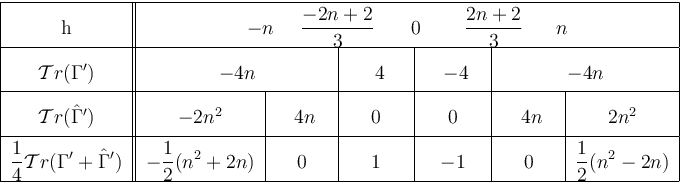
Now that we have evaluated the operators , , we can easily evaluate . The results are shown in Figure 3 and in Figure 3. In particular, we obtain
| (4.37) |
for . This agrees with the result in the commutative theory (4.6). As we mentioned at the beginning of subsection 4.2, this result can also be obtained from the arguments of subsection 3.3 for . Note also that we obtain both positive and negative topological charge, while we could define only negative charge in the previous formulation, as we pointed out in (2.29). Furthermore, we have obtained the results for non-admissible regions as well. The result (4.37) holds even in the non-admissible regions of , but it changes its value if we further extend the value of .

Since the chirality operator , (4.36), is independent of except for the prefactor, it can be written as
| (4.38) |
The other chirality operator is written as
| (4.39) |
Therefore, the GW Dirac operator (3.7) reduces to
| (4.40) |
for . Here is the GW Dirac operator of the previous definition (2.12), for the TP monopole configuration with magnetic charge (2.17)77 7 Incidentally, can be written as .. is independent of . is given in (4.34). This result (4.40) agrees with the commutative case (4.10).
5 Conclusions and Discussions
In this paper, we studied the topological structure of spontaneously symmetry-broken gauge theory on the fuzzy 2-sphere, by examining the index theorem which is applicable to general configurations, not restricted to a special type of configurations. We showed in detail that the commutative limit of the topological charge becomes the appropriate one introduced by ’t Hooft. Since this formulation is valid for general configurations, configuration space can be classified into topological sectors.
We then discussed the conditions to assure the validity of this formulation, which gave both upper and lower bounds to the fluctuations, though the ordinary admissibility condition in the lattice gauge theory gives only the upper bound. It is an interesting future problem to devise a mechanism which dynamically realizes these conditions rather than imposing them by hand. For example, we can deform the bosonic action to prevent configurations which are prohibited by these conditions [47]. This will open possibilities to perform Monte Carlo simulations of this formulation.
We also studied some topological properties of the topological charge. In particular, we showed that the topological charge is rewritten as the winding number of the scalar field in the noncommutative theory as well as in the commutative theory. We also found the gauge invariant and topologically invariant quantity, , in the noncommutative theory, whose counterpart in the commutative theory is absent. This quantity is related to the index of the would-be species-doubler. Although it is an analogue of a lattice artifact, it plays an important role in defining the index consistently in theories with finite degrees of freedom.
We further investigated some explicit configurations. We calculated the topological charge and obtained the simple form of the GW Dirac operator for these configurations. The results agree with the commutative case if the configurations satisfy the admissibility conditions. We also showed that we can define both positive and negative topological charge, while in the previous formulation we could only define the negative charge. We further obtained the results for non-admissible regions. Furthermore, since we obtained the explicit form of the Dirac operator for these configurations, we can calculate various quantities as the spectrum of the Dirac operator. While here we studied a series of configurations which connect the topological sectors with the topological charge and , it is also interesting to study configurations of other sectors. In order to study the configurations with the topological charge greater than or equal to , however, it may be necessary to obtain another representation of the configurations where space and gauge field are written separately.
We finally give some comments on the implications to the string theory compactifications. While in the general formulation studied in this paper, all of the topological sectors are defined from a single theory as in the commutative theories, defining the projective module in the noncommutative theory gives only a single topological sector, as in the previous formulation for the TP monopoles using the projection operator. This feature of the noncommutative theory, if we use it in the compactified spaces in the string theories, may be useful to determine the number of matter generations. On the other hand, we have observed various topological sectors in the non-admissible regions, from the calculations for the explicit configurations. They are different from the so-called noncommutative solitons and fluxons [53], which are also new topological objects in the noncommutative theory but appear only in the single topological sector specified by the theory. In the compactified spaces in the string theories, the notion of the ordinary space may be spoiled and the description of finite size matrices may become more appropriate. In these cases, the novel topologies in the non-admissible regions may play an important role in determining matter contents on our spacetime. We hope that the finite matrix will give a new possibility for the string theory compactifications.
Appendix A Commutative limit of the electric charge operator
In this appendix, we show that the electric charge operator becomes the normalized scalar field in the commutative limit, (3.3).
Since we consider the gauge group, the gauge field has the part and the part as
| (A.1) |
where the first term is of . Here we will assume that the part is of order one and the part is of .
Then, the scalar field
| (A.2) |
has the part of order one and the part of . The square of (A.2) becomes
| (A.3) |
In this form, the second term is of order one and the other terms are of .
The reason why we assumed that the part is negligibly small is for the normalization of . This assumption has nothing to do with the admissibility conditions, discussed in subsection 3.2, which assure the validity of the formulation. It is then desirable to define a more elaborate , which has the proper commutative limit without any constraints to the configurations.
Appendix B Commutative limit of the Dirac operator and the topological charge
In this appendix, we show the calculations of taking the commutative limit of the Dirac operator, (3.8), and the topological charge, (3.12).
The denominator of the chirality operator can be written as
| (B.1) |
since and . The second term in (B.1) is of the order of . We thus obtain
| (B.2) |
For taking the commutative limit of the Dirac operator , it is enough to take the first term in (B.2) into account. We can easily see
| (B.3) | |||||
| (B.4) |
In particular, in the gauge, it becomes the Dirac operator with the coupling to the unbroken gauge fields.
For taking the commutative limit of the topological charge, however, we have to take into account the second term in (B.2) as well. We then have
| (B.5) |
Note that the first and the second terms are of the order of , and give finite values after taking the trace, since taking trace gives a factor . The first term becomes in the commutative limit
| (B.6) |
as in [20, 26]. is the field strength defined as , where is the tangental components of the gauge field on the sphere. The second term becomes
| (B.7) |
where is a trace over the spinor space and over the gauge group space. is the covariant derivative operator defined as . Here we used
| (B.8) |
Taking the trace , (B.7) becomes
| (B.9) |
Therefore, the commutative limit of the topological charge becomes
| (B.10) |
which is precisely the topological charge introduced by ’t Hooft [44].
Appendix C Analyses on zero-modes in the chirality operators
In this appendix, we investigate zero-modes in the chirality operators and to obtain the results (4.25) and (4.36).
C.1 Bases and unitary transformations
As we mentioned below (4.24), there exists a two-folded degeneracy in the sector. We thus have an ambiguity to choose two multiplets, which we will call and . We here introduce three types of the bases with : are diagonalized by a spin operator and have spin respectively. Similarly, are diagonalized by with spin . are diagonalized by with spin . Therefore, these states are eigenstates for the following operators:
Different types of bases are related to one another by unitary transformation
| (C.10) |
The unitary matrices have the following forms:
This can be checked by comparing the highest-weight state, namely the state with , in each multiplet:
C.2 Calculations for zero-modes in
We now study zero-modes for the operator of (4.12). The zero-mode equation is written as
| (C.23) |
The state of is a simultaneous eigenstate for the operators in both sides of (C.23). The lhs gives , while the rhs gives . Therefore state becomes a zero-mode at . Similarly, the state becomes a zero-mode at .
For the states , we consider a linear combination . We here took the basis . From (C.1) and (C.1), (C.23) is written as
| (C.24) |
By taking as
| (C.25) |
(C.24) becomes
| (C.26) |
This equation has a nontrivial solution if and only if
| (C.27) |
is satisfied. This is satisfied by some real value if . On the other hand, by comparing (C.25) with (C.1), we have
| (C.28) |
and thus we obtain
| (C.29) |
for . Consequently, the states do not have zero-modes for an arbitrary real value if .
Therefore, we obtain our result (4.25).
C.3 Calculations for zero-modes in
We next consider zero-modes in . From Figure 1, we see that for , and are written as
We here took the bases . The unitary matrix relates to which are eigenstates of the operator of (4.12) with positive and negative eigenvalues.
Then, from (3.5), we obtain
| (C.42) |
For the block X of the sector, we have to evaluate a sign of the coefficient in
| (C.43) |
Here we took as
| (C.44) |
For , the operator becomes , and thus the basis reduces to . Then becomes , and we obtain
| (C.45) |
for . Similarly, we can obtain , and .
We then study whether takes place within the regions . means . This corresponds to the case where
| (C.46) |
is satisfied at some value of . By using
(C.46) is written as
Solving this equation, we obtain
| (C.69) | |||||
| (C.70) |
For , take positive and negative values respectively, which is consistent with the result in the previous subsection: has always positive and negative eigenvalues in the sector, since it does not have zero-modes for an arbitrary value of . Moreover, since for , does not take place within the region .
Since the operator is a continuous function of , so is . Thus has always the same sign in the region . Since has a negative value at , it always has negative values in this region. Therefore, we obtain our result (4.36).
References
- [1] T. Banks, W. Fischler, S. H. Shenker and L. Susskind, Phys. Rev. D 55, 5112 (1997) [arXiv:hep-th/9610043].
- [2] N. Ishibashi, H. Kawai, Y. Kitazawa and A. Tsuchiya, Nucl. Phys. B 498, 467 (1997) [arXiv:hep-th/9612115]. For a review: H. Aoki, S. Iso, H. Kawai, Y. Kitazawa, A. Tsuchiya and T. Tada, Prog. Theor. Phys. Suppl. 134, 47 (1999) [arXiv:hep-th/9908038].
- [3] A. Connes, Noncommutative geometry, Academic Press, 1990.
- [4] A. Connes, M. R. Douglas and A. Schwarz, JHEP 9802, 003 (1998) [arXiv:hep-th/9711162].
- [5] H. Aoki, N. Ishibashi, S. Iso, H. Kawai, Y. Kitazawa and T. Tada, Nucl. Phys. B 565, 176 (2000) [arXiv:hep-th/9908141].
- [6] N. Seiberg and E. Witten, JHEP 9909 (1999) 032 [arXiv:hep-th/9908142].
- [7] H. Grosse, C. Klimcik and P. Presnajder, Commun. Math. Phys. 178, 507 (1996) [arXiv:hep-th/9510083]; S. Baez, A. P. Balachandran, B. Ydri and S. Vaidya, Commun. Math. Phys. 208, 787 (2000) [arXiv:hep-th/9811169]; G. Landi, J. Geom. Phys. 37, 47 (2001) [arXiv:math-ph/9905014].
- [8] A. P. Balachandran and S. Vaidya, Int. J. Mod. Phys. A 16, 17 (2001) [arXiv:hep-th/9910129].
- [9] P. Valtancoli, Mod. Phys. Lett. A 16, 639 (2001) [arXiv:hep-th/0101189].
- [10] H. Steinacker, Nucl. Phys. B 679, 66 (2004) [arXiv:hep-th/0307075].
- [11] D. Karabali, V. P. Nair and A. P. Polychronakos, Nucl. Phys. B 627, 565 (2002) [arXiv:hep-th/0111249].
- [12] U. Carow-Watamura, H. Steinacker and S. Watamura, J. Geom. Phys. 54, 373 (2005) [arXiv:hep-th/0404130].
- [13] M. F. Atiyah and I. M. Singer, Annals Math. 93, 139 (1971).
- [14] K. Y. Kim, B. H. Lee and H. S. Yang, Phys. Rev. D 66, 025034 (2002) [arXiv:hep-th/0205010].
- [15] P. H. Ginsparg and K. G. Wilson, Phys. Rev. D 25, 2649 (1982).
- [16] H. Neuberger, Phys. Lett. B 417, 141 (1998) [arXiv:hep-lat/9707022]; Phys. Rev. D 57, 5417 (1998) [arXiv:hep-lat/9710089]; Phys. Lett. B 427, 353 (1998) [arXiv:hep-lat/9801031].
- [17] P. Hasenfratz, Nucl. Phys. Proc. Suppl. 63, 53 (1998) [arXiv:hep-lat/9709110]; P. Hasenfratz, V. Laliena and F. Niedermayer, Phys. Lett. B 427, 125 (1998) [arXiv:hep-lat/9801021].
- [18] M. Lüscher, Phys. Lett. B 428, 342 (1998) [arXiv:hep-lat/9802011].
- [19] F. Niedermayer, Nucl. Phys. Proc. Suppl. 73, 105 (1999) [arXiv:hep-lat/9810026].
- [20] H. Aoki, S. Iso and K. Nagao, Phys. Rev. D 67, 085005 (2003) [arXiv:hep-th/0209223].
- [21] J. Madore, Class. Quant. Grav. 9, 69 (1992).
- [22] A. P. Balachandran, T. R. Govindarajan and B. Ydri, Mod. Phys. Lett. A 15, 1279 (2000) [arXiv:hep-th/9911087]; arXiv:hep-th/0006216.
- [23] J. Nishimura and M. A. Vazquez-Mozo, JHEP 0108, 033 (2001) [arXiv:hep-th/0107110].
- [24] S. Iso and K. Nagao, Prog. Theor. Phys. 109, 1017 (2003) [arXiv:hep-th/0212284].
- [25] A. P. Balachandran and G. Immirzi, Phys. Rev. D 68, 065023 (2003) [arXiv:hep-th/0301242].
- [26] H. Aoki, S. Iso and K. Nagao, Nucl. Phys. B 684, 162 (2004) [arXiv:hep-th/0312199].
- [27] H. Aoki, S. Iso and T. Maeda, Phys. Rev. D 75, 085021 (2007) [arXiv:hep-th/0610125]. For a short review: H. Aoki, Prog. Theor. Phys. Suppl. 171, 228 (2007) [arXiv:0706.3078 [hep-th]].
- [28] H. Aoki, S. Iso, T. Maeda and K. Nagao, Phys. Rev. D 71, 045017 (2005) [arXiv:hep-th/0412052]
- [29] R. C. Myers, JHEP 9912, 022 (1999) [arXiv:hep-th/9910053].
- [30] S. Iso, Y. Kimura, K. Tanaka and K. Wakatsuki, Nucl. Phys. B 604, 121 (2001) [arXiv:hep-th/0101102].
- [31] P. Aschieri, T. Grammatikopoulos, H. Steinacker and G. Zoupanos, JHEP 0609, 026 (2006) [arXiv:hep-th/0606021]; H. Steinacker and G. Zoupanos, JHEP 0709, 017 (2007) [arXiv:0706.0398 [hep-th]].
- [32] S. Bal and H. Takata, Int. J. Mod. Phys. A 17, 2445 (2002) [arXiv:hep-th/0108002].
- [33] P. Valtancoli, Int. J. Mod. Phys. A 18, 967 (2003) [arXiv:hep-th/0206075].
- [34] T. A. Imai, Y. Kitazawa, Y. Takayama and D. Tomino, Nucl. Phys. B 665, 520 (2003) [arXiv:hep-th/0303120].
- [35] T. Azuma, S. Bal, K. Nagao and J. Nishimura, JHEP 0405, 005 (2004) [arXiv:hep-th/0401038]; JHEP 0605, 061 (2006) [arXiv:hep-th/0405277]; T. Azuma, K. Nagao and J. Nishimura, JHEP 0506, 081 (2005) [arXiv:hep-th/0410263].
- [36] P. Castro-Villarreal, R. Delgadillo-Blando and B. Ydri, Nucl. Phys. B 704, 111 (2005) [arXiv:hep-th/0405201].
- [37] M. Panero, JHEP 0705, 082 (2007) [arXiv:hep-th/0608202].
- [38] U. Carow-Watamura and S. Watamura, Commun. Math. Phys. 183, 365 (1997) [arXiv:hep-th/9605003]; Commun. Math. Phys. 212, 395 (2000) [arXiv:hep-th/9801195].
- [39] H. Grosse and J. Madore, Phys. Lett. B 283, 218 (1992); H. Grosse and P. Presnajder, Lett. Math. Phys. 33, 171 (1995); H. Grosse, C. Klimcik and P. Presnajder, Commun. Math. Phys. 185, 155 (1997) [arXiv:hep-th/9507074]; arXiv:hep-th/9603071.
- [40] H. Grosse and P. Presnajder, arXiv:hep-th/9805085; Lett. Math. Phys. 46, 61 (1998).
- [41] P. Presnajder, J. Math. Phys. 41, 2789 (2000) [arXiv:hep-th/9912050].
- [42] H. Aoki, S. Iso and K. Nagao, Phys. Rev. D 67, 065018 (2003) [arXiv:hep-th/0209137].
- [43] G. Ishiki, S. Shimasaki, Y. Takayama and A. Tsuchiya, JHEP 0611, 089 (2006) [arXiv:hep-th/0610038]; T. Ishii, G. Ishiki, S. Shimasaki and A. Tsuchiya, JHEP 0705, 014 (2007) [arXiv:hep-th/0703021]; Phys. Rev. D 77, 126015 (2008) [arXiv:0802.2782 [hep-th]].
- [44] G. ’t Hooft, Nucl. Phys. B 79, 276 (1974).
- [45] M. Luscher, Commun. Math. Phys. 85, 39 (1982).
- [46] P. Hernandez, K. Jansen and M. Luscher, Nucl. Phys. B 552, 363 (1999) [arXiv:hep-lat/9808010].
- [47] M. Luscher, Nucl. Phys. B 538, 515 (1999) [arXiv:hep-lat/9808021]; Nucl. Phys. B 549, 295 (1999) [arXiv:hep-lat/9811032].
- [48] K. Nagao, Phys. Rev. D 73, 065002 (2006) [arXiv:hep-th/0509034].
- [49] J. Arafune, P. G. O. Freund and C. J. Goebel, J. Math. Phys. 16, 433 (1975).
- [50] K. Fujikawa, Phys. Rev. D 60, 074505 (1999) [arXiv:hep-lat/9904007].
- [51] H. Aoki, J. Nishimura and Y. Susaki, JHEP 0702, 033 (2007) [arXiv:hep-th/0602078]; JHEP 0710, 024 (2007) [arXiv:hep-th/0604093].
- [52] H. Aoki, J. Nishimura and Y. Susaki, appear soon.
- [53] R. Gopakumar, S. Minwalla and A. Strominger, JHEP 0005, 020 (2000) [arXiv:hep-th/0003160]; J. A. Harvey, P. Kraus and F. Larsen, JHEP 0012, 024 (2000) [arXiv:hep-th/0010060]; N. Nekrasov and A. Schwarz, Commun. Math. Phys. 198, 689 (1998) [arXiv:hep-th/9802068]; A. P. Polychronakos, Phys. Lett. B 495, 407 (2000) [arXiv:hep-th/0007043]; D. J. Gross and N. A. Nekrasov, JHEP 0010, 021 (2000) [arXiv:hep-th/0007204]; M. Aganagic, R. Gopakumar, S. Minwalla and A. Strominger, JHEP 0104, 001 (2001) [arXiv:hep-th/0009142]; D. Bak, Phys. Lett. B 495, 251 (2000) [arXiv:hep-th/0008204]; D. J. Gross and N. A. Nekrasov, JHEP 0007, 034 (2000) [arXiv:hep-th/0005204].