Kinetic transport in the two-dimensional periodic Lorentz gasThanks: J.M. has been supported by EPSRC Research Grants GR/T28058/01 and GR/S87461/01, and a Philip Leverhulme Prize. A.S. is a Royal Swedish Academy of Sciences Research Fellow supported by a grant from the Knut and Alice Wallenberg Foundation.

One of the central challenges in kinetic theory is the derivation of macroscopic evolution equations—describing for example the dynamics of an electron gas—from the underlying fundamental microscopic laws of classical or quantum mechanics. An iconic mathematical model in this research area is the Lorentz gas [15], which describes an ensemble of non-interacting point particles in an infinite array of spherical scatterers. In the case of a disordered scatterer configuration, well known results by Gallavotti [12], Spohn [22], and Boldrighini, Bunimovich and Sinai [5] show that the time evolution of a macroscopic particle cloud is governed, in the limit of small scatterer density (Boltzmann-Grad limit), by the linear Boltzmann equation. We have recently proved an analogous statement for a periodic configuration of scatterers [16], [17]. In this case the linear Boltzmann equation fails (cf. also Golse [13]), and the random flight process that emerges in the Boltzmann-Grad limit is substantially more complicated.

In the present paper we focus on the two-dimensional case, and derive explicit formulae for the collision kernels of the limiting random flight process. These include information not only of the velocity before and after the collision (as in the case of the linear Boltzmann equation), but also the path length until the next hit and the velocity thereafter. Our formulae thus generalize those for the limiting distributions of the free path length found by Dahlqvist [10], Boca, Gologan and Zaharescu [3], and Boca and Zaharescu [4]. The higher dimensional case is more difficult, and we refer the reader to [16], [17], [18] for further information. The asymptotic estimates for the distribution tails in [18] improve the bounds by Bourgain, Golse and Wennberg [6].

Our results on the Boltzmann-Grad limit complement classical studies in ergodic theory, where the scatterer size remains fixed. Bunimovich and Sinai [7] showed that the dynamics of the two-dimensional periodic Lorentz gas is diffusive in the limit of large times, and satisfies a central limit theorem. They assumed that the periodic Lorentz gas has a finite horizon, i.e., the scatterers are configured in such a way that the path length between consecutive collisions is bounded. The corresponding result for infinite horizon has recently been established by Szasz and Varju [21] following initial work by Bleher [2]. See also the recent papers by Dolgopyat, Szasz and Varju [11], and Melbourne and Nicol [19], [20] for related studies of statistical properties of the two-dimensional periodic Lorentz gas. The case of higher dimensions is still open, even for models with finite horizon, cf. Chernov [9], and Balint and Toth [1]. Scaling limits that are intermediate between the Boltzmann-Grad and the limit of large times have been explored by Klages and Dellago [14].

—–

This paper is organized as follows. We begin by recalling the necessary details from [16], [17], then derive our main results—the explicit formulae for the collision kernels of the two-dimensional Lorentz gas in the Boltzmann-Grad limit. The final two sections study the implications for the distribution of free path lengths, and asymptotic properties of the collision kernels.

—–

To describe the main results of [16], [17], let us fix a euclidean lattice ${\mathcal{L}}\subset{\mathbb{R}}^{d}$, and assume (without loss of generality) that its fundamental cell has volume one. We denote by ${\mathcal{K}}_{\rho}\subset{\mathbb{R}}^{d}$ the complement of the set ${\mathcal{B}}_{\rho}^{d}+{\mathcal{L}}$ (the “billiard domain”), and $\operatorname{T{}}^{1}({\mathcal{K}}_{\rho})={\mathcal{K}}_{\rho}\times\operatorname{S{}}_{1}^{d-1}$ its unit tangent bundle (the “phase space”), with ${\text{\boldmath$q$}}\in{\mathcal{K}}_{\rho}$ the position and ${\text{\boldmath$v$}}\in\operatorname{S{}}_{1}^{d-1}$ the velocity of the particle. Here ${\mathcal{B}}_{\rho}^{d}$ denotes the open ball of radius $\rho$, centered at the origin, and $\operatorname{S{}}_{1}^{d-1}$ the unit sphere. The dynamics of a particle in the Lorentz gas is defined as the motion with unit speed along straight lines, and specular reflection at the balls ${\mathcal{B}}_{\rho}^{d}+{\mathcal{L}}$. (We will here also permit more general scattering processes.) In order to pass to the Boltzmann-Grad limit, it is convenient to rescale the length units in such a way that the mean free path length remains constant as $\rho\to 0$. This is achieved by introducing the macroscopic coordinates $({\text{\boldmath$x$}},{\text{\boldmath$v$}})=(\rho^{d-1}{\text{\boldmath$q$}},{\text{\boldmath$v$}})\in\operatorname{T{}}^{1}(\rho^{d-1}{\mathcal{K}}_{\rho})$.

We take $({\text{\boldmath$x$}}_{0},{\text{\boldmath$v$}}_{0})\in\operatorname{T{}}^{1}(\rho^{d-1}{\mathcal{K}}_{\rho})$ as the initial data, and denote by $\tau_{1}({\text{\boldmath$x$}}_{0},{\text{\boldmath$v$}}_{0})$ the time until the first collision (the free path length), ${\text{\boldmath$v$}}_{1}({\text{\boldmath$x$}}_{0},{\text{\boldmath$v$}}_{0})$ the velocity thereafter, and analogously by $\tau_{k}({\text{\boldmath$x$}}_{0},{\text{\boldmath$v$}}_{0})$ and ${\text{\boldmath$v$}}_{k}({\text{\boldmath$x$}}_{0},{\text{\boldmath$v$}}_{0})$ the time between the $(k-1)$st and $k$th collision and the subsequent velocity. The following theorem proves the existence of a joint limiting distribution for random initial data in the limit $\rho\to 0$. The statement is a variant of the more general Theorem 4.1 in [17].

The collision kernels $p({\text{\boldmath$v$}}_{0},\xi_{1},{\text{\boldmath$v$}}_{1})$ and $p_{\mathbf{0},{\text{\boldmath$\beta$}}_{{\text{\boldmath$v$}}_{0}}^{+}}({\text{\boldmath$v$}}_{1},\xi_{2},{\text{\boldmath$v$}}_{2})$ are in particular independent of the choice of $\Lambda$ and ${\mathcal{L}}$, and are characterized in [16], [17] by certain measures on the homogeneous spaces $\operatorname{ASL}(d,{\mathbb{Z}})\backslash\operatorname{ASL}(d,{\mathbb{R}})$ and $\operatorname{SL}(d,{\mathbb{Z}})\backslash\operatorname{SL}(d,{\mathbb{R}})$, respectively. In the present paper we will show how, in dimension $d=2$, this abstract description can be turned into explicit, elementary formulae; the same task seems substantially more difficult in dimension $d>2$.

Theorem 1 forms the key ingredient in the proof of the existence of a stochastic process that governs the particle dynamics in the limit $\rho\to 0$, see [17] for details. Specifically, a particle cloud with initial density $f_{0}$ evolves in time $t$ to the density $f_{t}$ given by

where $f$ is the unique solution of the differential equation

subject to the initial condition $f(0,{\text{\boldmath$x$}},{\text{\boldmath$v$}},\xi,{\text{\boldmath$v$}}_{+})=f_{0}({\text{\boldmath$x$}},{\text{\boldmath$v$}})p({\text{\boldmath$v$}},\xi,{\text{\boldmath$v$}}_{+})$. Equation (3) may be viewed as a substitute for the linear Boltzmann equation, which describes the macroscopic dynamics in a random, rather than periodic, configuration of scatterers [12], [22], [5]. Independently of our studies in [16], [17], Caglioti and Golse [8] have recently proposed an equation analogous to (3) in dimension $d=2$, by assuming an independence hypothesis which is analogous to the statement of Theorem 1 above.

—–

In order to treat more general scattering processes than specular reflection, we recall the basic facts from [17, Section 2.2], limiting our attention to the case $d=2$. For a scatterer centered at the lattice point ${\text{\boldmath$m$}}\in{\mathcal{L}}\subset{\mathbb{R}}^{2}$, we use the boundary coordinates $({\text{\boldmath$v$}},{\text{\boldmath$w$}})\in\operatorname{S{}}_{1}^{1}\times\operatorname{S{}}_{1}^{1}$, where $v$ is the velocity and $w$ position so that ${\text{\boldmath$q$}}={\text{\boldmath$m$}}+\rho{\text{\boldmath$w$}}$. Let

be the set of incoming data at a given scatterer, i.e., the relative velocity and position at the time of collision. The corresponding outgoing data is parametrized by the set

We define the scattering map by

In the case of the original Lorentz gas the scattering map is given by specular reflection,

Let $\Theta_{1}({\text{\boldmath$v$}},{\text{\boldmath$w$}})\in\operatorname{S{}}_{1}^{1}$ and $\Theta_{2}({\text{\boldmath$v$}},{\text{\boldmath$w$}})\in\operatorname{S{}}_{1}^{1}$ be the projection of $\Theta({\text{\boldmath$v$}},{\text{\boldmath$w$}})\in\operatorname{S{}}_{1}^{1}$ onto the first and second component, respectively. We assume in the following that

1. (i)

   the scattering map $\Theta$ is spherically symmetric, i.e., if $({\text{\boldmath$v$}}_{+},{\text{\boldmath$w$}}_{+})=\Theta({\text{\boldmath$v$}},{\text{\boldmath$w$}})$ then $({\text{\boldmath$v$}}_{+}K,{\text{\boldmath$w$}}_{+}K)=\Theta({\text{\boldmath$v$}}K,{\text{\boldmath$w$}}K)$ for all $K\in\operatorname{O{}}(2)$;

2. (ii)

   if ${\text{\boldmath$w$}}=-{\text{\boldmath$v$}}$ then ${\text{\boldmath$v$}}_{+}=-{\text{\boldmath$v$}}$;

3. (iii)

   $\Theta:{\mathcal{S}}_{-}\to{\mathcal{S}}_{+}$ is $\operatorname{C{}}^{1}$ and for each fixed ${\text{\boldmath$v$}}\in\operatorname{S{}}_{1}^{1}$ the map ${\text{\boldmath$w$}}\mapsto\Theta_{1}({\text{\boldmath$v$}},{\text{\boldmath$w$}})$ is a $\operatorname{C{}}^{1}$ diffeomorphism from $\{{\text{\boldmath$w$}}\in\operatorname{S{}}_{1}^{1}\>:\>{\text{\boldmath$v$}}\cdot{\text{\boldmath$w$}}<0\}$ onto some open subset of $\operatorname{S{}}_{1}^{1}$.

We will write $\varphi({\text{\boldmath$v$}},{\text{\boldmath$u$}})\in[0,2\pi)$ for the angle between any two vectors ${\text{\boldmath$v$}},{\text{\boldmath$u$}}\in\mathbb{R}^{2}\setminus\{\mathbf{0}\}$, measured counter-clockwise from $v$ to $u$. Using the spherical symmetry and $\Theta_{1}({\text{\boldmath$v$}},-{\text{\boldmath$v$}})=-{\text{\boldmath$v$}}$ one sees that there exists a constant $0\leq B_{\Theta}<\pi$ such that for each ${\text{\boldmath$v$}}\in\operatorname{S{}}_{1}^{1}$, the image of the diffeomorphism ${\text{\boldmath$w$}}\mapsto\Theta_{1}({\text{\boldmath$v$}},{\text{\boldmath$w$}})$ is

Let us write ${\text{\boldmath$\beta$}}_{\text{\boldmath$v$}}^{-}:{\mathcal{V}}_{\text{\boldmath$v$}}\to\{{\text{\boldmath$w$}}\in\operatorname{S{}}_{1}^{1}\>:\>{\text{\boldmath$v$}}\cdot{\text{\boldmath$w$}}<0\}$ for the inverse map. Then ${\text{\boldmath$\beta$}}_{\text{\boldmath$v$}}^{-}$ is spherically symmetric in the sense that ${\text{\boldmath$\beta$}}_{{\text{\boldmath$v$}}K}^{-}({\text{\boldmath$u$}}K)={\text{\boldmath$\beta$}}_{{\text{\boldmath$v$}}}^{-}({\text{\boldmath$u$}})K$ for all ${\text{\boldmath$v$}}\in\operatorname{S{}}_{1}^{1}$, ${\text{\boldmath$u$}}\in{\mathcal{V}}_{\text{\boldmath$v$}}$, $K\in\operatorname{O{}}(2)$, and in particular ${\text{\boldmath$\beta$}}_{\text{\boldmath$v$}}^{-}({\text{\boldmath$u$}})$ is jointly $\operatorname{C{}}^{1}$ in ${\text{\boldmath$v$}},{\text{\boldmath$u$}}$.

We also define

The map ${\text{\boldmath$\beta$}}^{+}$ is spherically symmetric and jointly $\operatorname{C{}}^{1}$ in ${\text{\boldmath$v$}},{\text{\boldmath$u$}}$. In terms of the original scattering situation, the point of our notation is the following: Given any ${\text{\boldmath$v$}}_{-},{\text{\boldmath$v$}}_{+}\in\operatorname{S{}}_{1}^{1}$, there exist ${\text{\boldmath$w$}}_{-},{\text{\boldmath$w$}}_{+}\in\operatorname{S{}}_{1}^{1}$ such that $\Theta({\text{\boldmath$v$}}_{-},{\text{\boldmath$w$}}_{-})=({\text{\boldmath$v$}}_{+},{\text{\boldmath$w$}}_{+})$ if and only if $B_{\Theta}<\varphi({\text{\boldmath$v$}}_{-},{\text{\boldmath$v$}}_{+})<2\pi-B_{\Theta}$, and in this case ${\text{\boldmath$w$}}_{-}$ and ${\text{\boldmath$w$}}_{+}$ are uniquely determined, as ${\text{\boldmath$w$}}_{\pm}={\text{\boldmath$\beta$}}^{\pm}_{{\text{\boldmath$v$}}_{-}}({\text{\boldmath$v$}}_{+})$. For example, in the case of specular reflection (7) we have $B_{\Theta}=0$ and

We denote the unit vectors $(1,0)$ and $(0,1)$ by ${\text{\boldmath$e$}}_{1}$ and ${\text{\boldmath$e$}}_{2}$, respectively. For ${\text{\boldmath$v$}}=(\cos\phi,\sin\phi)\in\operatorname{S{}}_{1}^{1}$ we set

so that ${\text{\boldmath$v$}}K({\text{\boldmath$v$}})={\text{\boldmath$e$}}_{1}$. The classical impact parameter is related to the above by

where $\vartheta=\varphi({\text{\boldmath$v$}},{\text{\boldmath$u$}})$. The scattering cross section is $\sigma(\vartheta)\equiv\sigma({\text{\boldmath$v$}},{\text{\boldmath$u$}})=|b^{\prime}(\vartheta)|$. We define the exit parameter correspondingly by

with $\vartheta=\varphi({\text{\boldmath$u$}},{\text{\boldmath$v$}})$.

In the case of specular reflection (7), we have $b(\vartheta)=\cos(\vartheta/2)$, $s(\vartheta)=-\cos(\vartheta/2)$.

—–

We now turn to the main results of this paper.

It follows that $\Phi_{\mathbf{0}}(\xi,w,z)$ is discontinuous at each point $(\xi,w,z)\in S$, where $S$ is the curve $S=\bigl\{((1+|z|)^{-1},-z,z)\>:\>-1<z<1\bigr\}$; in fact $\Phi_{\mathbf{0}}$ maps any neighbourhood of such a point onto the interval $[0,1]$. On the other hand $\Phi_{\mathbf{0}}$ is continuous everywhere in the complementary region, $(\xi,w,z)\in\bigl(\mathbb{R}_{>0}\times(-1,1)\times(-1,1)\bigr)\setminus S$.

We now turn to the proof of Theorem 2, which will involve computations similar to those in [23, Sec. 8].

—–

The inner integral in (25) evaluates to

To state the result of the second integration in (25), we define the auxiliary function $\Psi(a)$ for $a>0$ as the solution to $\Psi^{\prime}(a)=(a^{-1}-1)\log\bigl|a^{-1}-1\bigr|$ with $\Psi(1)=0$; thus

with the dilogarithm $\operatorname{Li}_{2}(z)=\sum_{k=1}^{\infty}\frac{z^{k}}{k^{2}}$ ($|z|\leq 1$). For $\xi$ in the range $\frac{1}{2}<\xi<\frac{1}{1+|w|}$ we set

and for $\xi$ in the range $\frac{1}{1+|w|}<\xi<\frac{1}{1-|w|}$ we set

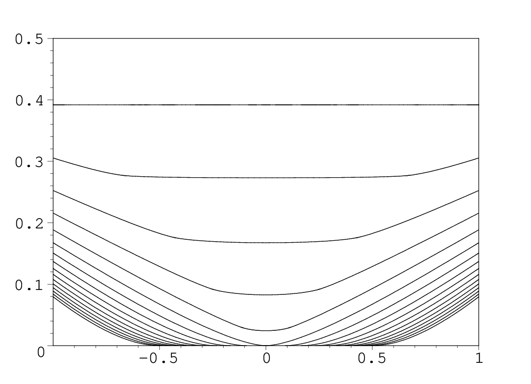
The density $\Phi(\xi,w)$ in (25) can now be written as

We have already seen in [16, Remark 4.5] that $\Phi(\xi,w)$ is continuous for all $(\xi,w)\in\mathbb{R}_{>0}\times(-1,1)$. The fact that the formulae on the right hand side of (30) agree at the points $\xi=\frac{1}{1+|w|}$ can be verified directly from (27)–(29), using the identity $\operatorname{Li}_{2}(\frac{1+|w|}{2})+\operatorname{Li}_{2}(\frac{1-|w|}{2})=-\log(\frac{1+|w|}{2})\log(\frac{1-|w|}{2})+\frac{\pi^{2}}{6}$. The function $\Phi(\xi,w)$ can furthermore be continuously extended to $\mathbb{R}_{>0}\times[-1,1]$ by setting

We finally remark that the function $\Phi(\xi,0)$ was computed in [23, Prop. 3] in a different context; set $\Phi(\xi,0)=f_{1}^{\text{box},\operatorname{SL}_{2}}(4\xi)$ in the notation of that paper.

—–

Dahlqvist [10], Boca, Gologan and Zaharescu [3], and Boca and Zaharescu [4] have obtained explicit formulae for the limiting distribution of the free path lengths in dimension two. These can be recovered from the above expressions via the relations (cf. [16, Remark 4.3])

for the free path length between consecutive collisions,

for the free path length from a generic initial point inside the billiard domain, and

for the free path length of a particle starting at a lattice point (with the scatterer removed).

—–

We conclude with a brief asymptotic analysis of the collision kernels, when $\xi\to\infty$ (the limit $\xi\to 0$ is trivial). We assume in the following that $\xi>1$. A short calculation shows that, if $wz\leq 0$, we have $\Phi_{\text{\boldmath$0$}}(\xi,w,z)=0$. Otherwise, for $wz>0$,

where $u=\xi(1-|w|)$, $y=\xi(1-|z|)$. Thus

uniformly with respect to $w,z\in(-1,1)$ as $\xi\to\infty$. A simple integration yields for (26)

We substitute $\eta=t\xi$ in (25) and apply (37) to obtain

if $u\in[0,1)$, and $\Phi(\xi,w)=0$ otherwise. Both (37) and (38) hold uniformly with respect to $w\in(-1,1)$ as $\xi\to\infty$. These asymptotics can of course also be obtained by expanding (26) and (30), respectively.

References

• [1] P. Balint and I.P. Toth, Exponential decay of correlations in multi-dimensional dispersing billiards, preprint 2007.
• [2] P.M. Bleher, Statistical properties of two-dimensional periodic Lorentz gas with infinite horizon. J. Statist. Phys. 66 (1992), 315–373.
• [3] F.P. Boca, R.N. Gologan and A. Zaharescu, The statistics of the trajectory of a certain billiard in a flat two-torus. Comm. Math. Phys. 240 (2003), 53-73.
• [4] F.P. Boca and A. Zaharescu, The distribution of the free path lengths in the periodic two-dimensional Lorentz gas in the small-scatterer limit, Commun. Math. Phys. 269 (2007), 425-471.
• [5] C. Boldrighini, L.A. Bunimovich and Y.G. Sinai, On the Boltzmann equation for the Lorentz gas. J. Statist. Phys. 32 (1983), 477–501.
• [6] J. Bourgain, F. Golse and B. Wennberg, On the distribution of free path lengths for the periodic Lorentz gas. Comm. Math. Phys. 190 (1998), 491–508.
• [7] L.A. Bunimovich and Y.G. Sinai, Statistical properties of Lorentz gas with periodic configuration of scatterers. Comm. Math. Phys. 78 (1980/81), 479–497.
• [8] E. Caglioti and F. Golse, The Boltzmann-Grad limit of the periodic Lorentz gas in two space dimensions, arXiv:0710.0716
• [9] N.I. Chernov, Statistical properties of the periodic Lorentz gas. Multidimensional case. J. Statist. Phys. 74 (1994), 11–53.
• [10] P. Dahlqvist, The Lyapunov exponent in the Sinai billiard in the small scatterer limit. Nonlinearity 10 (1997), 159–173.
• [11] D. Dolgopyat, D. Szasz and T. Varju, Recurrence properties of the planar Lorentz process, Duke Math. J., to appear.
• [12] G. Gallavotti, Divergences and approach to equilibrium in the Lorentz and the Wind-tree-models, Physical Review 185 (1969), 308–322.
• [13] F. Golse, On the periodic Lorentz gas and the Lorentz kinetic equation, preprint arXiv:math/0703812.
• [14] R. Klages and C. Dellago, Density-dependent diffusion in the periodic Lorentz gas, J. Stat. Phys. 101 (2000), 145–159.
• [15] H. Lorentz, Le mouvement des électrons dans les métaux, Arch. Néerl. 10 (1905), 336–371.
• [16] J. Marklof and A. Strömbergsson, The distribution of free path lengths in the periodic Lorentz gas and related lattice point problems, arXiv:0706.4395; to appear in the Annals of Mathematics.
• [17] J. Marklof and A. Strömbergsson, The Boltzmann-Grad limit of the periodic Lorentz gas, arXiv:0801.0612
• [18] J. Marklof and A. Strömbergsson, The periodic Lorentz gas in the Boltzmann-Grad limit: Asymptotic estimates. In preparation.
• [19] I. Melbourne and M. Nicol, Almost sure invariance principle for nonuniformly hyperbolic systems. Comm. Math. Phys. 260 (2005), 131–146.
• [20] I. Melbourne and M. Nicol, A vector-valued almost sure invariance principle for hyperbolic dynamical systems, arXiv:math/0606535
• [21] D. Szasz and T. Varju, Limit laws and recurrence for the planar Lorentz process with infinite horizon, preprint 2007.
• [22] H. Spohn, The Lorentz process converges to a random flight process, Comm. Math. Phys. 60 (1978), 277–290.
• [23] A. Strömbergsson, A. Venkatesh, Small solutions to linear congruences and Hecke equidistribution, Acta Arith., 118 (2005), 41-78.