Classical solutions for the Carroll-Field-Jackiw-Proca electrodynamics

For a purely timelike background, $V^{\alpha}=(\mathbf{v}_{0},\mathbf{0}),$ the components of the inverse tensor operator, $\left[D_{\nu\beta}\right]^{-1}$, takes the form

where $\epsilon_{123}=1$ and $\Delta$ is

We are interested in stationary solution of the four-potential, thus, setting $p_{0}=0$ the components of the tensor $\left[D_{\nu\beta}\right]^{-1}$ read as

with

We should now write a general expression for the four-potential by the Green method taking a non-null current density. In this sense, the four-potential is read as

where $G_{\mu\nu}\left(\mathbf{r}-\mathbf{r}^{\prime}\right)$ is the Green’s functions here written in terms of the inverse tensor $\left[\bar{D}^{-1}\right]_{\mu\nu}$:

From the matrix $\left[\bar{D}^{-1}\right]_{\mu\nu}\left(\mathbf{p}\right),$ we can write straightforwardly the components of the Green function in terms of Fourier integrals:

where the integrals $I_{i}\left(\mathbf{R}\right)$ are defined bellow:

where $\mathbf{R}=\left(\mathbf{r}-\mathbf{r}^{\prime}\right)$. In order to solve these integrals, we first have factorized the denominator as $\ \left(\mathbf{p}^{2}+M_{A}^{2}\right)^{2}-\mathbf{v}_{0}^{2}\mathbf{p}^{2}=\left(\mathbf{p}^{2}-m_{+}^{2}\right)\left(\mathbf{p}^{2}-m_{-}^{2}\right)$. It is very important to remark that the massive poles $m_{\pm}^{2},$

are positive under the condition $\mathbf{v}_{0}^{2}\geqslant 4M_{A}^{2}$. This fact is responsible for the oscillatory character of the magnetic sector solutions to be achieved for this model. The remaining three integrals can be solved in the complex plane, yielding:

with

Replacing these results in eq. (31), the Green function $G_{jk}\left(\mathbf{r}-\mathbf{r}^{\prime}\right)$ is finally obtained:

where $\Delta_{jk}=\left(\delta_{kj}-3R_{j}R_{k}/R^{2}\right)$. This Green function can be simplified to its MCFJ counterpart taking the limit $\left(M_{A}\rightarrow 0\right)$:

It is easy to verify that such result in the Lorentz symmetric limit ($\mathbf{v}_{0}\rightarrow 0)$ rescues the pure Maxwell result

Turning back to the issue of calculating explicit classical solutions, we address the solution for the scalar potential. Regarding eq. (27), and the density current for a point-like charge, $J_{0}\left(\mathbf{r}\right)=e\delta\left(\mathbf{r}\right)$, the following expression is obtained for the scalar potential

where $r=\left|\left|\mathbf{r}\right|\right|$. The electric field may be easily evaluated from the scalar potential ($\mathbf{E}=-\nabla A_{0}),$ exhibiting an exponentially decaying solution as well:

It is interesting to note that this is the same result obtained for the electric field of the Maxwell-Proca Lagrangian (without Lorentz violation, $V^{\mu}=0$). This means that the Lorentz-violating background, when coupled to the gauge field as in Lagrangian (1), does not alter the electrostatic sector. Analysis of Maxwell equations (4,5,6) in the static regime reveals that this scenario remains true even in the presence of a non-null current. Hence, the scalar potential and electric field achieved here are the same for a point-like charge in uniform motion (stationary solution), once the current $\mathbf{J}$ does not contribute to $A_{0}$. In the absence of the Proca mass, the solutions (44, 45) reduce to the CFJ ones, which coincide with the Coulombian result:

The fixed background, therefore, does to not induce any effect on the electric field solution of the MCFJ model, as well. This fact deserves to be compared with the scenario of the dimensionally reduced version of this model, studied in ref. [17]. In such work, it was shown that the purely timelike background alters the character of the classical Maxwell-Chern-Simons electric solution, turning the usual screened Bessel-like solution into an unscreened $1/r$ electric field.

The solution for vector potential can be found by the same procedure. From the inverse tensor $\left[D_{\nu\beta}\right]^{-1}$, we obtain the expression for the vector potential Fourier transform:

where it was considered that $\mathbf{\tilde{J}}\cdot\mathbf{p}=0$, as a consequence of current conservation $(p_{\alpha}\tilde{J}^{\alpha}=0)$. In this case, we take the current associated with a point-like charge in uniform motion with velocity $\mathbf{u}$,

In the momentum space, $\mathbf{\tilde{J}}\left(\mathbf{p}\right)\mathbf{=}e\mathbf{u}$. The vector potential, written as the Fourier transform of eq. (47), may be compactly expressed in terms of the integrals (37,39), so that:

Considering the results already obtained, the vector potential takes the form:

where $A_{\pm}=a_{\pm}/a$. For the case of a vanishing Proca mass ($M_{A}\rightarrow 0)$, this expression is reduced to the MCFJ vector solution:

It is interesting to note that oscillating solutions are obtained in both cases, and the Proca mass is not a factor able to annihilate such a behavior. For the case of a point-like static charge, the potential vector and the magnetic field strength are null, once it depends only on the current source $\left(\mathbf{j}\neq 0\right)$. Hence, for a point-like charge in uniform motion, $~\mathbf{J}\left(\mathbf{r}\right)=e\mathbf{u}\delta\left(\mathbf{r}\right),$ the magnetic field becomes non-null. It can be derived from the vector potential $\left(\mathbf{B}=\nabla\times\mathbf{A}\right)$, yielding:

An additional contribution proportional to $\left(\mathbf{u\cdot r}\right)\mathbf{r}$ also appears in the above expression, but it is was discarded because the scalar product $\mathbf{u\cdot r}$ is null. This result stems from the condition $\nabla\cdot\mathbf{A=0,}$ a consequence of the external current conservation in the stationary regime. This magnetic field solution exhibits two components: one in the direction the velocity $\mathbf{u}$, and another orthogonal to the plane defined by $\mathbf{u}$ and $\mathbf{r.}$ This magnetic field exhibits a decaying $1/r^{2}$ behavior both near the origin ($r\rightarrow 0)$ and asymptotically. In the limit of a vanishing Proca mass ($M_{A}\rightarrow 0),$ this expression is reduced to the MCFJ solution:

This solution, similarly to the MCFJ-Proca one, is also decomposed in terms of two orthogonal directions, $\mathbf{u}$ and $\mathbf{u}\times\mathbf{r}$. The fact that the MCFJ magnetic field exhibits an oscillating behavior, associated with the $1/r^{2}$ behavior of the MCFJ electric field, is compatible with the emission of Cerenkov radiation by a point-like charge in uniform motion [9]. At the same way, the exponentially decaying behavior of eq. (45) puts in evidence that no Cerenkov radiation can be emitted by a stationary charge in the framework of the MCFJ-Proca electrodynamics, once one condition to have radiation is that the fields should present a non null asymptotic behavior [9].

Another regime in which such solutions shall be investigated is the one of a vanishing LV background ($\mathbf{v}_{0}\rightarrow 0),$ which should lead back to the usual Maxwell-Proca electrodynamics. This limit, however, can not be implemented directly on the MCFJ-Proca expressions of eqs. (50,52), since these solutions were derived under the condition $\mathbf{v}_{0}^{2}\geqslant 4M_{A}^{2}$, which assures that the poles (36) be real and positive definite. A way to avoid this complication is to implement the limit $\mathbf{v}_{0}\rightarrow 0$ on eqs. (51,53). The results obtained,

nonetheless, do not recover the correct Maxwell-Proca behavior,

attained from $\tilde{\mathbf{A}}_{i}\left(p\right)=-\tilde{J}_{i}/\left(\mathbf{p}^{2}+M_{A}^{2}\right)$ [eq. (47) taken in the limit $\mathbf{v}_{0}\rightarrow 0$]. This apparent non equivalence simply shows that Maxwell-Proca behavior may not be found as the limit $\mathbf{v}_{0}\rightarrow 0\mathbf{\ }$of the MCFJ-Proca solutions. This is ascribed to the structure of poles appearing in the MCFJ model, $1/\left(\mathbf{p}^{2}+m^{2}\right)$, associated with an exponentially decaying behavior, in contrast with the MCFJ-Proca pole structure, $1/\left(\mathbf{p}^{2}-m^{2}\right),$ related to an oscillating behavior. In this way, we see that the background turns the exponentially decaying behavior of the Maxwell-Proca model into a oscillating solution that goes as $1/r^{2}$ far from the origin. This is true in both MCFJ and MCFJ-Proca models.

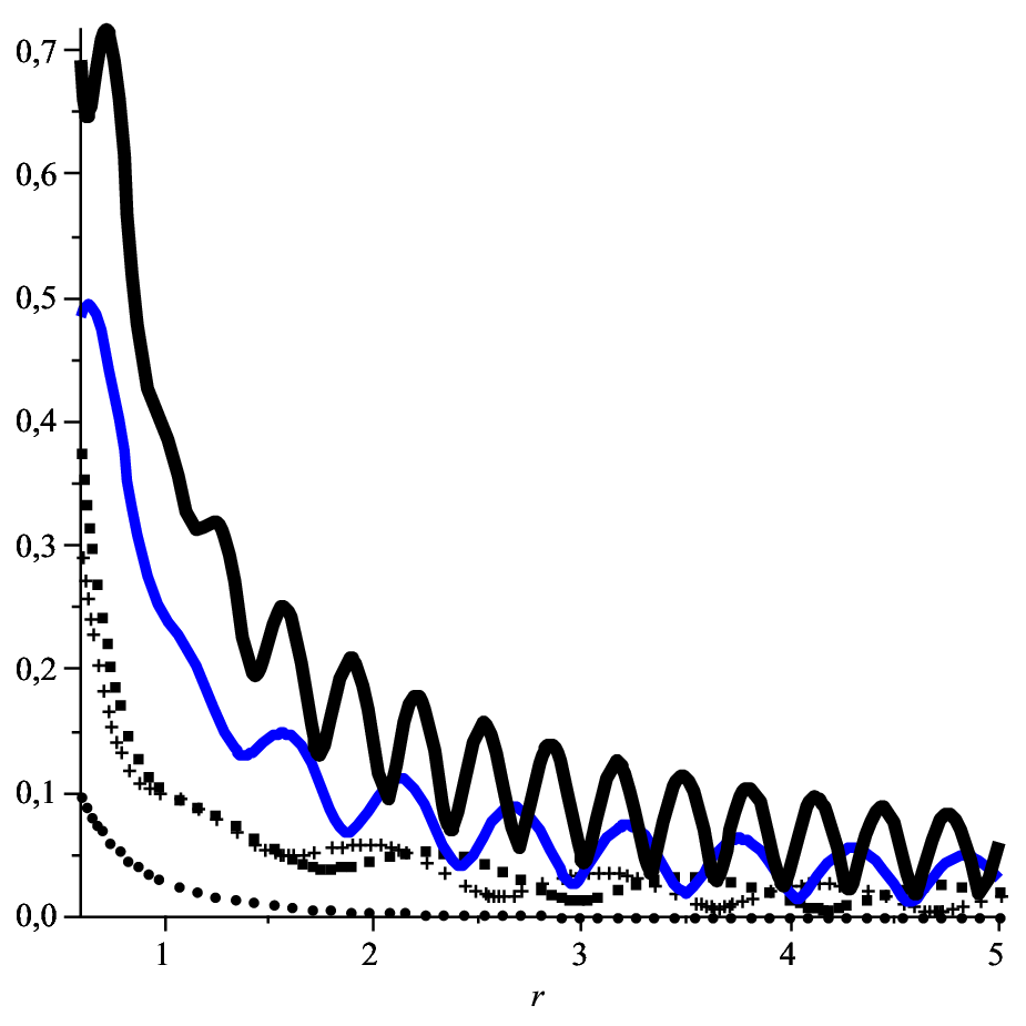
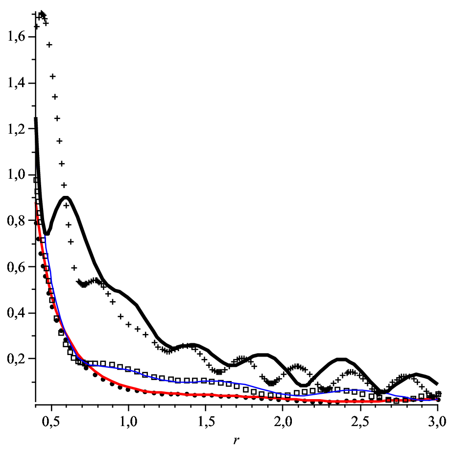
The graph of Fig.1 depicts a simultaneous plot of the Maxwell-Proca, MCFJ and MCFJ-Proca magnetic fields in the case the velocity $\mathbf{u}$ is orthogonal to the vector $\mathbf{r}$. Such a graph shows clearly that the MCFJ-Proca solution deviates substantially from the Maxwell-Proca behavior mainly due to the presence of oscillation. This deviation increases with the background magnitude: the larger is the background, more pronounced is the amplitude and the frequency of such oscillations. For a background not so large in comparison with the Proca mass $\left(\mathbf{v}_{0}\gtrsim M_{A}\right)$, the MCFJ e MCFJ-Proca solutions are close from each other. Keeping $M_{A}$ constant while $\mathbf{v}_{0}$ increases, it occurs that these solutions become different. This behavior is confirmed in the graph of Fig.2, where it is shown a comparison between the MCFJ and MCFJ-Proca magnetic solutions for equal values of $\mathbf{v}_{0}$ (for the case the velocity $\mathbf{u}$ is orthogonal to the vector $\mathbf{r).}$ In general, these solutions are nearly coincident, but deviate from each other for larger $M_{A}$ magnitudes.

In order to find a general expression for the magnetic field strength, a direct way consists in starting from wave equation (8), which in the stationary regime and for a purely timelike background is simplified to:

The corresponding Green function for this equation is $G\left(\mathbf{r}-\mathbf{r}^{\prime}\right)=\!\!\displaystyle\int\frac{d^{3}\mathbf{p}}{\left(2\pi\right)^{3}}\,\tilde{G}\left(\mathbf{p}\right)e^{i\mathbf{p}\cdot\left(\mathbf{r}-\mathbf{r}^{\prime}\right)},$ with $\tilde{G}\left(p\right)=[\left(\mathbf{p}^{2}-m_{+}^{2}\right)\left(\mathbf{p}^{2}-m_{-}^{2}\right)]^{-1},$ and the poles $m_{\pm}^{2}$ being given by eq. (36). In true, this Green function was already evaluated, corresponding to the result of integral $I_{3}$, so that the magnetic field strength is:

This outcome differs from the MCFJ one presented in ref. [10], which exhibits an exponentially decaying behavior. For the case of the pure CFJ model ($M_{A}\rightarrow 0)$, we get:

with $R=\left|\left|\mathbf{r-r}^{\prime}\right|\right|$. Using the Green theorem, $\int_{V}\left[\phi\mathbf{\nabla}^{2}\chi-\chi\mathbf{\nabla}^{2}\phi\right]d^{3}r=\int_{\partial R}\left[\phi\partial\chi/\partial n-\chi\partial\phi/\partial n\right]dS$, and considering that the current and its derivatives are null on a very distant surface, then eq. (58) is rewritten as:

where it was used $\nabla^{2}[(1-\cos($v${}_{0}R))/R]=\mathbf{v}_{0}^{2}\cos(\mathbf{v}_{0}R)/R$. This result is equal to the one of ref. [10] apart from a global signal stemming from our definition of the external current vector $\mathbf{j}\left(\mathbf{r}\right)$.

The case the background is purely spacelike, $V^{\alpha}=\left(0,\mathbf{v}\right),$ becomes particularly interesting when we consider the model of Lagrangian (1) under the perspective of its physical consistency. In fact, it is known that this model exhibits full consistency (stability, causality, unitarity) only for a spacelike background. Henceforth, this is a good reason to study the corresponding classical solutions for a purely spacelike background. We begin writing the elements of the inverse matrix (19) for $V^{\alpha}=\left(0,\mathbf{v}\right)$:

with $D=\left({p}^{2}-M_{A}^{2}\right)^{2}-\mathbf{v}^{2}p^{2}-\left(\mathbf{v\cdot p}\right)^{2}$.

As we are to study the stationary solutions of the model, we set $p_{0}=0$ in the above equations to get the Green function for the wave equation for the stationary four potential:

where

Supposing that $\theta$ is the angle between the vectors $\mathbf{p}$ and $\mathbf{v}$, ($\mathbf{p}\cdot\mathbf{v=|p||v|\cos}\theta)$, the denominator $R_{s}$ is read as:

Similarly to the timelike case, we can construct the stationary Green function from the inverse matrix (64). In this sense, we write:

where the Fourier transforms $F_{i}$ are defined as: