Geodesic manifolds with a transitive subset of smooth biLipschitz maps

Enrico Le Donne Address: Yale University, Mathematics Dept., PO Box 208283, New Haven, CT 06520-8283 Email address: enrico.ledonne@yale.edu

Abstract.

This paper is connected with the problem of describing path metric spaces that are homeomorphic to manifolds and biLipschitz homogeneous, i.e., whose biLipschitz homeomorphism group acts transitively.

Our main result is the following. Let $X=G/H$ be a homogeneous manifold of a Lie group $G$ and let $d$ be a geodesic distance on $X$ inducing the same topology. Suppose there exists a subgroup $G_{S}$ of $G$ that acts transitively on $X$ , such that each element $g\in G_{S}$ induces a locally biLipschitz homeomorphism of the metric space $(X,d)$ . Then the metric is locally biLipschitz equivalent to a sub-Riemannian metric. Any such metric is defined by a bracket generating $G_{S}$ -invariant sub-bundle of the tangent bundle.

The result is a consequence of a more general fact that requires a transitive family of uniformly biLipschitz diffeomorphisms with a control on their differentials. It will be relevant that the group acting transitively on the space is a Lie group and so it is locally compact, since, in general, the whole group of biLipschitz maps, unlikely the isometry group, is not locally compact.

Our method also gives an elementary proof of the following fact. Given a Lipschitz sub-bundle of the tangent bundle of a Finsler manifold, then both the class of piecewise differentiable curves tangent to the sub-bundle and the class of Lipschitz curves almost everywhere tangent to the sub-bundle give rise to the same Finsler-Carnot-Carathéodory metric, under the condition that the topologies induced by these distances coincide with the manifold topology.

1. Introduction

In the last 20 years there has been a surge of interest in the geometry of non-smooth spaces and in their corresponding biLipschitz analysis. This movement arose from the interaction between active areas of mathematics concerning the theory of Analysis on Metric Spaces [Sem96, HK98, Che99, AK00, LP01, Hei01, Laa02], Geometric Analysis [GS92, BGP92, CC97] along with Geometric Group Theory, Rigidity, and Quasiconformal Homeomorphisms. One focus of this research has been the study of mappings between non-Riemannian metric structures such as Carnot groups and boundaries of hyperbolic groups [Pan89, BM91, MM95, KL97, Gro99, BP00, KB02].

In the present paper, we focus on the rigidity of certain non-smooth metric structures on manifolds, namely, geodesic metrics on manifolds that have a transitive group of biLipschitz homeomorphisms; for short they are called biLipschitz homogeneous geodesic manifolds. Every known example is locally biLipschitz equivalent to a homogeneous space $G/H$ equipped with a Carnot-Carathéodory metric; here $G$ is a connected Lie group and $H$ is a closed subgroup. Any such metric, also called a sub-Riemannian metric, is defined by a bracket generating sub-bundle of the tangent bundle, also known as completely non-holonomic distribution. For surveys of this area, including how the jargon interchanges between sub-Riemannian geometry and Carnot-Carathéodory geometry, see [BBI01, Mon02] and the papers [Gro96, Mit85, Bel96].

All of the $2$ -dimensional examples, known so far, are locally biLipschitz equivalent to the Euclidean plane. One may therefore ask whether these are in fact the only examples. Our main goal in this paper is to show that under additional assumptions this is indeed the case.

The motivation for this question comes from several sources. First, one can view this as an analogue, in the biLipschitz category, of Hilbert’s fifth problem on the characterization of Lie groups, solved in [MZ74], or the conjectural Bing-Borsuk characterization of topological manifolds. Another source of motivation is the work of Berestovskiĭ [Ber88, Ber89a, Ber89b], who showed that a finite dimensional geodesic metric space with transitive isometry group is isometric to an example $G/H$ as above, except that in the general case one has to use a Finsler-Carnot-Carathéodory metric as opposed to a Riemannian-Carnot-Carathéodory metric. In addition, a coarse version of this question in the two dimensional case has arisen in several situations in Geometric Group Theory, and is directly related with the problem considered. For example in [KK06], with the purpose of analyzing $2$ -dimensional Poincaré duality groups over commutative rings, Michael Kapovich and Bruce Kleiner studied quasi-homogeneous quasi-planes, i.e., simply-connected metric cell complexes satisfying a coarse Poincaré duality in dimension $2$ on which the group of quasi-isometries acts transitively. Quasi-planes also appeared in [KK05].

We consider length metrics since otherwise there are many metrics with transitive isometry group that are not locally biLipschitz to the standard one, e.g., even on the real line $\mathbb{R}$ , all distances $d(s,t):=\sqrt[d]{|s-t|}$ , for $d>1$ , are translation invariant. In fact, biLipschitz homogeneous curves have been studied deeply in [Bis01, GH99].

We show that, locally, the examples mentioned above are the only examples if the biLipschitz maps giving homogeneity come from a Lie group acting by diffeomorphisms. This assumption is equivalent to the space being homeomorphic to a homogeneous space $X=G/H$ , with $G$ containing a transitive subgroup of biLipschitz homeomorphisms. To be precise, we prove the following:

Theorem 1.1.

Let $G$ be a Lie group and $H$ be a closed subgroup. Let $X=G/H$ be the corresponding homogeneous manifold equipped with a geodesic distance $d$ inducing its natural topology. Suppose there exists a subgroup $G_{S}$ of $G$ that acts transitively on $X$ , and that acts by maps that are locally biLipschitz with respect to $d$ . Then there exists a completely non-holonomic $G_{S}$ -invariant distribution, such that any Carnot-Carathéodory metric coming from it gives a metric that is locally biLipschitz equivalent to $d$ .

Notice that we do not assume uniform bounds on the biLipschitz constants. Indeed, if one assumes that $X$ is a geodesic metric space with a transitive group $G$ of $L$ -biLipschitz homeomorphisms, then by taking the supremum over the $G$ -orbit of the distance function, and then the associated path metric, one gets an $L$ -biLipschitz equivalent metric with respect to which $G$ acts by isometries. One can then apply Berestovskiĭ’s result in [Ber89b] mentioned above. However, without the extra hypothesis about uniformity of biLipschitz constants, the argument breaks down altogether. Our work can be considered as the first step toward a coarse version of Berestovskiĭ’s result. In fact, the main steps of our proof and Berestovskiĭ’s strategy share some common features, although his method is more algebraic.

Our assumption is connected with the fact that, in general, the full group of biLipschitz maps is not a locally compact group. On the other hand, as a consequence of the Ascoli-Arzelà Theorem, the isometry group of the space $X$ is a locally compact topological group. Berestovskiĭ uses this fact in the case that the isometry group acts transitively to apply the celebrated Gleason-Montgomery-Zippin Theorem and subsequent work [MZ74, Chapter III]. The result is a reduction to the case when the action of the isometry group is topologically conjugate to a transitive smooth action of a Lie group on a smooth manifold, in fact on a homogeneous space $X=G/H$ . Thus, in the case of biLipschitz homogeneous geodesic manifolds, we shall assume that we already have a similar structure, in the sense that the biLipschitz maps giving homogeneity are coming from a Lie group $G$ acting on a quotient $G/H$ .

Since the problem is in fact local, another formulation is as follows. Suppose we have a geodesic metric on a neighborhood of the origin in $\mathbb{R}^{n}$ , and a collection of biLipschitz maps that sends the origin to any point in this neighborhood. Furthermore, suppose that these biLipschitz maps are, in fact, elements of a smooth “local” action. Then we can conclude that in a neighborhood of the origin this metric is biLipschitz equivalent to a Carnot-Carathéodory metric. See the next section for more general statements.

Here is a concrete application of Theorem 1.1.

Example: Affine maps giving homogeneity.

Suppose we have a geodesic distance on the plane such that for any two points there exists an affine map that is locally biLipschitz with respect to the geodesic distance and sends the first point to the second. Then we can conclude that the distance is locally biLipschitz equivalent to the Euclidean one.

Indeed, one can apply Theorem 1.1 where $G$ is the group of affine diffeomorphisms and $H=GL_{2}(\mathbb{R})$ . The group $G_{S}$ is the intersection between $G$ and the group of maps that are locally biLipschitz with respect to $d$ . The metric is in fact Riemannian since there is no proper sub-Riemannian structures in dimension $2$ .

Several references [Ber88, Gro96, Mon02] state that in the definition of Carnot-Carathéodory metrics, one gets the same metric when considering either piecewise continuously differentiable, or Lipschitz (or absolutely continuous curves), as horizontal curves. However, we could not find any proof of this fact in the literature. An element of the proof of Theorem 1.1, detailed in step 5 below, can be used to give a simple proof of this fact in the case that the two topologies are assumed to coincide. See the Appendix for details.

Theorem 1.2.

Let $X$ be a Finsler manifold, equipped with a locally Lipschitz sub-bundle (of the tangent bundle). Then both the class of piecewise $C^{1,1}$ curves tangent to the sub-bundle and the class of Lipschitz curves almost everywhere tangent to the sub-bundle give rise to the same Finsler-Carnot-Carathéodory metric, under the condition that the topologies induced by these distances coincide with the manifold topology.

1.1. An outline of the proof of Theorem 1.1

Step 1.

Argue that we can assume that the group $G$ is embedded and closed in the homeomorphism group of the space $X=G/H$ . Thus, every time we will apply the Ascoli-Arzelà theorem, the limits of $C^{0}$ -converging subsequences will still be elements of the group and the convergence will be, in fact, $C^{\infty}$ .
Step 2.

Apply a Baire category argument to get a locally transitive set of elements of the group that are $C^{k}$ close to ${\rm id}_{X}$ and are uniformly biLipschitz with respect to both the metric $d$ and any Riemannian metric on $X$ that we fixed.
Step 3.

Prove that, locally, the distance $d$ is greater than a multiple of some smooth Riemannian distance. Therefore, the geodesics for $d$ are Lipschitz maps for the smooth distance; thus, they are differentiable almost everywhere.
Step 4.

Define a sub-bundle of the tangent bundle related to the set of velocities of the geodesics. Use it to define a Carnot-Carathéodory metric $d_{CC}$ . It will be easy to argue that $d\geq{\rm Constant}\cdot d_{CC}$ locally.
Step 5.

Prove that $d\leq{\rm Constant}\cdot d_{CC}$ locally.

1.2. Organization of the paper

In the next section, we discuss generalizations and variations of Theorem 1.1., Indeed, steps 3, 4, and 5 above constitute a more general fact, specified in Theorem 2.1, that implies Theorem 1.1. In Section 3, we show that locally the distance $d$ is greater than a multiple of any smooth distance. An immediate consequence is the absolute continuity of geodesics: any curve that is rectifiable with respect to the geodesic distance $d$ is differentiable almost everywhere. In Section 4, we define a subset of the tangent bundle, and prove that it is, in fact, a sub-bundle; this allows us to define an associated Carnot-Carathéodory metric. In Section 5, we prove the biLipschitz equivalence between the geodesic metric $d$ , and the newly defined Carnot-Carathéodory metric. In Section 6, we complete steps 1 and 2 above to show how Theorem 1.1 follows from Theorem 2.1. In Appendix A, we repeat the argument to prove Theorem 1.2.

Acknowledgements

It is a pleasure to thank the Department of Mathematics of Yale University for the warm and friendly atmosphere that I am enjoying during my Ph.D. program. Above all, I particularly wish to thank Bruce Kleiner for his confidence and support.

2. The general criterion and some consequences

Theorem 1.1 is a consequence of a more general fact. Given a geodesic metric on a domain in $\mathbb{R}^{n}$ , whenever there is a transitive family of uniformly biLipschitz diffeomorphisms with a control on their differentials, then the metric is locally biLipschitz equivalent to a Carnot-Carathéodory metric. Namely, this conclusion can be reached when there is a family $\mathcal{F}$ of $C^{2}$ -diffeomorphisms and a base point $p_{0}$ such that the orbit $\mathcal{F}(p_{0})$ is a neighborhood of $p_{0}$ , the elements of $\mathcal{F}$ are uniformly biLipschitz for both the distance $d$ and a fixed Riemannian metric, and the family of the differentials has a uniform modulus of continuity.

We will denote by $\left\|A\right\|_{{\rm Lin}(\mathbb{R}^{n})}$ the norm as linear operator of a matrix $A\in{\rm Lin}(\mathbb{R}^{n})$ .

Theorem 2.1.

Let $N\subset\mathbb{R}^{n}$ be a compact neighborhood of $0\in\mathbb{R}^{n}$ , equipped with a geodesic distance $d$ that induces the standard topology. Suppose there exists a family $\mathcal{F}\subset C^{2}(N,\mathbb{R}^{n})$ of local $C^{2}$ -diffeomorphisms satisfying:

Homogeneity:

for any $p\in N$ , there is $f\in\mathcal{F}$ , so that $f(0)=p$ ;

Uniform biLipschitz:

there exists $k\in\mathbb{R}$ such that each $f\in\mathcal{F}$ is a $k$ -biLipschitz map on $N\cap f^{-1}(N)$ , with respect to both the Euclidean metric and the distance $d$ ;

Uniform modulus of continuity of derivatives:

the family $\{df\}_{f\in\mathcal{F}}$ has a uniform modulus of continuity, i.e., there exists an increasing function $\eta:[0,\infty)\to[0,\infty)$ , with $\eta(0)=0$ , so that, for any $f\in\mathcal{F}$ and $x,y\in N$ ,

(2.1)

\left\|(df)_{x}-(df)_{y}\right\|_{{\rm Lin}(\mathbb{R}^{n})}\leq\eta(|x-y|);

Then there exists an $\mathcal{F}$ -invariant, $C^{1}$ sub-bundle $\Delta\subset TN$ such that if $d_{\Delta}$ is any sub-Riemannian metric coming from $\Delta$ , then the geodesic metric $d$ is locally biLipschitz equivalent to $d_{\Delta}$ .

The conclusion of the above theorem is that the regularity of the bundle is $C^{1}$ . However, we will prove that the distribution of Theorem 1.1 is smooth in Proposition 6.8.

The following variation shows how Theorem 2.1 can be used:

Theorem 2.2.

Let $d$ be a geodesic metric on a neighborhood $N$ of the origin in $\mathbb{R}^{n}$ . Suppose that there exists a $C^{2}$ map

	$\displaystyle F:\Lambda\times U$	$\displaystyle\to$	$\displaystyle N$
	$\displaystyle(\lambda,p)$	$\displaystyle\mapsto$	$\displaystyle F_{\lambda}(p),$

where $U\subset N\subset\mathbb{R}^{n}$ and $\Lambda\subset\mathbb{R}^{N}$ are neighborhoods of the origin, with the property that, for some neighborhood of the origin $\Lambda_{0}\subset\Lambda$ , the set

\{F_{\lambda}(0):F_{\lambda}\text{ is biLipschitz w.r.t. }d,\,\lambda\in\Lambda_{0}\}

is a neighborhood of the origin. Then in a (possible smaller) neighborhood of the origin the metric $d$ is biLipschitz equivalent to a Carnot-Carathéodory metric.

Proof.

Clearly, we may assume $F_{0}={\rm id}_{U}$ , and $U$ and $\Lambda_{0}$ compact sets. We want to show that the hypotheses of Theorem 2.1 apply. Indeed, first, since the map $F$ is $C^{2}$ , the condition about the family of differentials having a uniform modulus of continuity is immediately verified. Next, call $m$ -biLipschitz those maps that are $m$ -biLipschitz with respect to both the Euclidean distance and the distance $d$ , and consider the sets

A_{m}:=\left\{p\in U\;:\;F_{\lambda}(0)=p,\;F_{\lambda}\;m\text{-biLipschitz },\,\lambda\in\Lambda_{0}\right\},

Each $A_{m}$ is closed. Indeed, take $F_{\lambda_{j}}(0)\in A_{m}\to p$ , with $F_{\lambda_{j}}$ an $m$ -biLipschitz map, then by Ascoli-Arzelà Theorem, some subsequence converges: $F_{\lambda_{j}}\to F$ uniformly and $F$ is still an $m$ -biLipschitz map. Since here we have assumed $\Lambda_{0}$ compact, $\lambda_{j}\to\lambda_{\infty}\in\Lambda_{0}$ up to subsequence, so $F=F_{\lambda_{\infty}}$ so $p\in A_{m}$ , i.e., $A_{m}$ is closed. So, by Baire Category Theorem, for some $m\in\mathbb{N}$ , the set $\{F_{\lambda}(0):F_{\lambda}\;m-\text{biLipschitz }\}$ is a neighborhood of a point in $U$ that we can assume to be the origin. Theorem 2.1 can be applied to conclude. ∎

We now give a generalization of Theorem 1.1 that points out the importance of the assumption that the group acting transitively on the space is a Lie group and so is locally compact. Notice that the whole group of biLipschitz maps, unlikely the isometry group, is not in general locally compact. According to Montgomery-Zippin’s work [MZ74], if a locally compact group acts continuously, effectively, and transitively on a manifold, then it is a Lie group, Here and in what follows, manifolds are supposed to be connected, however, Lie groups can have infinitely many components. Thus, Theorem 1.1 yields the following generalization:

Theorem 2.3.

Let $(M,d)$ be a manifold endowed with a geodesic metric (inducing the same topology). Let $G$ be a locally compact group with a countable base. Let $G\times M\to M$ be a continuous, effective action of $G$ on $M$ . Suppose there exists a subgroup of $G$ acting transitively on $M$ by biLipschitz maps (with respect to the metric $d$ ). Then $(M,d)$ is locally biLipschitz equivalent to a homogeneous space equipped with a Carnot-Carathéodory metric.

Proof.

Following, [MZ74], any locally compact group $G$ has the property of having an open subgroup $G^{\prime}<G$ that is the inverse limit of Lie groups; with the language of Montgomery-Zippin’s book, $G^{\prime}$ has property $A$ .

First, we claim that, for any $q\in M$ , the orbit of $q$ under $G^{\prime}$ , $G^{\prime}\cdot q$ , is open. This is because, called $H$ the stabilizer of the action, the projection $G\to G/H$ is open and the orbit action $G/H\to M$ is an homeomorphism by an standard argument [Hel01, page 121, Theorem 3.2].

Now we show that the $G^{\prime}$ -action is still transitive. Indeed, fix a point $p\in M$ , suppose by contradiction that $G^{\prime}\cdot p\neq M$ . Hence,

M=\left(G^{\prime}\cdot p\right)\bigsqcup\left(\bigcup_{q\notin G^{\prime}\cdot p}G^{\prime}\cdot q\right)

is a disjoint union of two non-empty open sets of $M$ . This contradicts the fact that $M$ is connected.

Thus $G^{\prime}$ satisfies the hypotheses of Montgomery-Zippin’s Theorem [MZ74, page 243], so $G^{\prime}$ is a Lie group. So $G^{\prime}$ doesn’t have small subgroups, thus neither does $G$ . By Gleason-Yamabe Theorem, cf. [MZ74, Chapter III], $G$ is a Lie group. ∎

3. The given metric is greater than a Riemannian metric

We now start the proof of Theorem 2.1. In particular this section is devoted to showing that curves that are rectifiable with respect to the geodesic distance $d$ , are differentiable almost everywhere. To prove this we will show (cf. Proposition 3.3) that the given metric $d$ is locally greater than a Riemannian metric.

We begin with a couple of lemmas. The first asserts that, if we just want $C^{1}$ maps, we may assume continuity of the differentials when the evaluation at a base point goes to the base point.

Lemma 3.1.

Under the assumptions of Theorem 2.1, there exists a family $\{f_{p}\}_{p\in N}\subset C^{1}(N,\mathbb{R}^{n})$ , satisfying $f_{p}(0)=p$ , that is uniformly biLipschitz, satisfies the condition that the family $\{df_{p}\}$ has a uniform modulus of continuity, and satisfies:

Continuity of $(df_{p})_{0}$ at $0$ :

the map

	$\displaystyle N$	$\displaystyle\to$	$\displaystyle{\rm Lin}(\mathbb{R}^{n})$
	$\displaystyle p$	$\displaystyle\mapsto$	$\displaystyle(df_{p})_{0}$

is continuous at $p=0$ . In other words,

(3.1)

\left\|(df_{0})_{0}-(df_{p})_{0}\right\|_{{\rm Lin}(\mathbb{R}^{n})}\to 0,\qquad\text{as }p\to 0.

Proof.

This is another application of the Baire Category Theorem. Set $A_{0}:=N$ . For each $j\in\mathbb{N}$ , let $\{V_{m}^{(j)}\}_{m\in\mathbb{N}}$ be a countable cover of ${\rm Lin}(\mathbb{R}^{n})$ by balls of diameter $<j^{-1}$ , with respect to some fixed metric inducing the standard topology. Inductively define sets $A_{j}\subseteq\mathbb{R}^{n}$ as follows. Let $\mathcal{F}$ be the family from Theorem 2.1 and let

A_{j,m}=\{p\in A_{j}:\exists f\in\mathcal{F},f(0)=p,(df)_{0}\in V^{(j)}_{m}\}.

Then $A_{j}=\cup_{m}A_{j,m}$ . By the Baire Category Theorem, there is $m_{j}\in\mathbb{N}$ so that there exists a ball $A_{j+1}$ of radius $<j^{-1}$ in the closure of $A_{j,m_{j}}$ . Let $q\in\cap_{j}A_{j}$ . By post-composing with a map that sends $q$ to $0$ we may assume that $q=0$ .

For any $p\neq 0$ in $N$ , we have $p\in A_{j}\setminus A_{j+1}$ , for some $j$ . Then we define $f_{p}$ as follows. Since $p\in A_{j}$ , there exists sequences $\{p_{k}\}\subseteq A_{j-1}$ , $\{f_{k}\}\subseteq\mathcal{F}$ such that $p_{k}\to p$ , $f_{k}(0)=p_{k}$ , and $(df_{k})_{0}\in V^{(j)}_{m_{j}}$ . Note that the functions $f_{k}$ are uniformly Lipschitz and converge at $0$ , and that the sequence $\{(df_{k})_{0}\}$ is equicontinuous and uniformly bounded at $0$ . Thus, by the Ascoli-Arzelà Theorem, a subsequence of $\{f_{k}\}$ converges in the $C^{1}$ topology. Let $f_{p}$ be one such limit. We can apply this same argument to any sequence $\{f_{p_{j}}\}$ with $p_{j}\to 0$ and define $f_{0}$ as one of the limits of some sequence $\{f_{p_{j_{i}}}\}$ converging in the $C^{1}$ topology. All of the constructed maps $f_{p}$ ’s are $C^{1}$ and still are uniformly biLipschitz and their derivatives have uniform modulus of continuity. Moreover, since $\cap_{j}V^{(j)}_{m_{j}}$ is a single point,

(df_{p})_{0}\to(df_{0})_{0},\quad\text{as }p\to 0.

∎

The next lemma gives uniform control on the deviation of elements in the family $\mathcal{F}$ from their linear approximations.

Lemma 3.2 (Uniform distortion control).

If a family $\mathcal{F}$ has the property that the family $\{df\}_{f\in\mathcal{F}}$ is equicontinuous, so (2.1) holds, then there exists an increasing function $\omega(t)$ such that, for any element $f\in\mathcal{F}$ and $y\in N$ ,

(3.2)

|(df)_{0}(y)+f(0)-f(y)|\leq\omega(|{y}|),

and $\dfrac{\omega(t)}{t}\to 0$ as $t\to 0$ .

Proof.

By assumption, there exists an increasing function $\eta:[0,\infty)\to[0,\infty)$ , with $\eta(0)=0$ , so that, for any $f\in\mathcal{F}$ and $x,y\in N$ ,

\left\|(df)_{x}-(df)_{y}\right\|_{{\rm Lin}(\mathbb{R}^{n})}\leq\eta(|x-y|).

Let $\omega(t):=\eta(t)t$ . Thus we just need to show (3.2) for any $f\in\mathcal{F}$ and $y\in N$ . Consider the function $t\in\mathbb{R}\mapsto f(ty)$ . By the Fundamental Theorem of Calculus and the Chain Rule,

f(y)-f(0)=\int_{0}^{1}\dfrac{d}{dt}f(ty)\,dt=\int_{0}^{1}(df)_{ty}\cdot y\,dt.

So,

$\displaystyle\|(df)_{0}(y)+f(0)-f(y)\|$	$\displaystyle\leq$	$\displaystyle\int_{0}^{1}\|(df)_{0}\cdot y-(df)_{ty}\cdot y\|\,dt$
	$\displaystyle\leq$	$\displaystyle\int_{0}^{1}\left\\|(df)_{0}-(df)_{ty}\right\\|\|y\|\,dt$
	$\displaystyle\leq$	$\displaystyle\int_{0}^{1}\eta(\|ty\|)\|y\|\,dt$
	$\displaystyle\leq$	$\displaystyle\int_{0}^{1}\eta(\|y\|)\|y\|\,dt$
	$\displaystyle=$	$\displaystyle\omega(\|{y}\|).$

∎

This next proposition is the core of the paper. We get the first important relation between the geodesic distance $d$ and the Euclidean metric.

Proposition 3.3.

Let $(N,d)$ satisfy the assumptions of Theorem 2.1. Then some multiple of the distance $d$ is greater than the Euclidean one, i.e., there exists $C>0$ such that

(3.3)

\left\|p-q\right\|\leq C\cdot d(p,q),

for any $p,q\in N$ .

Proof.

It suffices to prove (3.3) for $p,q$ in a neighborhood $V_{0}$ of the origin. Indeed, since the family $\mathcal{F}$ acts transitively by $k$ -biLipschitz maps with respect to both metrics, then we would have that any point $p\in N$ has a neighborhood $V$ where $\left\|q_{1}-q_{2}\right\|\leq Ck^{2}d(q_{1},q_{2}),$ for $q_{1},q_{2}\in V$ . Indeed, let $f\in\mathcal{F}$ so that $f(0)=p$ . Then, for any $q_{1},q_{2}\in V:=f(V_{0})$ , we have

\left\|q_{1}-q_{2}\right\|\leq k\left\|f^{-1}(q_{1})-f^{-1}(q_{2})\right\|\leq Ckd\left(f^{-1}(q_{1}),f^{-1}(q_{2})\right)\leq Ck^{2}d(q_{1},q_{2}).

Now, since both distances are geodesic, we would conclude $\left\|p-q\right\|\leq Ck^{2}d(p,q),$ for all points $p,q\in N$ .

Suppose (3.3) is not true. So there is a sequence of pairs of points $p_{n},q_{n}$ where the ratio of the metrics is smaller and smaller:

\dfrac{d(p_{n},q_{n})}{\left\|p_{n}-q_{n}\right\|}<\dfrac{1}{n},

for all $n\in\mathbb{N}$ . We can assume $q_{n}=0$ , since we can move it to $0$ using the transitivity of $k$ -biLipschitz maps. Indeed, let $f_{n}$ be a $k$ -biLipschitz diffeomorphism such that $f_{n}(q_{n})=0$ , for each $n\in\mathbb{N}$ . Now,

\dfrac{1}{n}>\dfrac{d(p_{n},q_{n})}{\left\|p_{n}-q_{n}\right\|}\geq\dfrac{\dfrac{1}{k}d(f_{n}(p_{n}),f_{n}(q_{n}))}{k\left\|f_{n}(p_{n})-f_{n}(q_{n})\right\|}=\frac{1}{k^{2}}\dfrac{d(f_{n}(p_{n}),0)}{\left\|f_{n}(p_{n})\right\|}.

After replacing $p_{n}$ with $f_{n}(p_{n})$ and possibly changing indices, we get a sequence of points $p_{n}\in N$ with the property

(3.4)

\dfrac{d(p_{n},0)}{\left\|p_{n}\right\|}<\dfrac{1}{n}.

Note that $p_{n}\to 0$ as $n\to\infty$ . Indeed, $p$ is in the bounded set $N$ , so $d(p_{n},0)\leq\frac{1}{n}\left\|p_{n}\right\|\leq\frac{1}{n}{\rm Diam}(N)\to 0$ . Moreover, $d$ gives the usual topology, so $p_{n}\to 0$ .

By Lemma 3.1, there is a neighborhood $U$ of $0$ such that

\left\|(df_{p})_{0}-(df_{0})_{0}\right\|_{{\rm Lin}(\mathbb{R}^{n})}\leq\dfrac{1}{4},\quad\forall p\in U.

Thus, since $f_{0}={\rm id}$ , we have, for any vector $v\in\mathbb{R}^{2}$ ,

(3.5)

\left\|(df_{p})_{0}(v)-v\right\|\leq\left\|(df_{p})_{0}-{\rm Id}\right\|_{{\rm Lin}(\mathbb{R}^{n})}\left\|v\right\|\leq\dfrac{1}{4}\left\|v\right\|\quad\forall p\in U.

All of the balls in the argument shall have the origin as center. Consider an Euclidean ball of radius $R$ contained in the neighborhood $U$ . Since the topologies induced by the two distances are the same, we can find a $d$ -ball of radius $r>0$ inside the Euclidean one. We want to use the fact that the points $p_{n}$ go to zero, and are different from $0$ , to construct a ‘pseudo’ geodesic as a chain of a controlled number of points, whose final point $H(p_{n})$ will be outside the $d$ ball of radius $r$ .

Let $\omega$ be the function from Lemma 3.2 that controls the extent to which maps in $\mathcal{F}$ fail to be linear at $0$ . Now, fix $n\in\mathbb{N}$ so large that $\omega(\left\|p_{n}\right\|)<\frac{1}{4}\left\|p_{n}\right\|.$ Since $p_{n}$ is now fixed, we will drop the subscript $p=p_{n}$ . Therefore by estimates (3.5) and (3.2), we have

(3.6)

\left\|p+f(0)-f(p)\right\|\leq\dfrac{1}{2}\left\|p\right\|,\quad\forall f\in\mathcal{F}.

Starting with $f_{0}={\rm id}$ , by recurrence, for $j\in\mathbb{N}$ , choose $f_{j}\in\mathcal{F}$ such that $f_{j}(0)=f_{j-1}(p)$ . We claim that there exists $j\leq\dfrac{2R}{\left\|p\right\|}$ for which $f_{j}(p)$ is not in the Euclidean ball of radius $R$ . In fact, each $f_{j}(p)$ is quantitatively farther from $0$ than $f_{j-1}(p)$ . Indeed, we consider the projection $\pi_{p}(f_{j}(p))$ of $f_{j}(p)$ on the direction of $p$ and prove that

(3.7)

\pi_{p}(f_{j}(p)):=\dfrac{\langle f_{j}(p)|p\rangle}{\left\|p\right\|}\geq\dfrac{j}{2}\left\|p\right\|.

We prove (3.7) by induction using the estimates (3.6) and the fact that $\langle u|v\rangle\geq\langle w|v\rangle-\left\|u-w\right\|\cdot\left\|v\right\|$ , for all $u,v,w\in\mathbb{R}^{2}$ . For $j=1$ ,

	$\displaystyle\langle f_{j}(p)\|p\rangle$	$\displaystyle\geq$	$\displaystyle\langle p+p\|p\rangle-\left\\|f_{1}(p)-p-p\right\\|\cdot\left\\|p\right\\|$
		$\displaystyle\geq$	$\displaystyle 2\left\\|p\right\\|^{2}-\frac{1}{2}\left\\|p\right\\|^{2}\geq\frac{1}{2}\left\\|p\right\\|^{2}.$

Assume (3.7) proved for $j$ , then

$\displaystyle\langle f_{j+1}(p)\|p\rangle$	$\displaystyle\geq$	$\displaystyle\langle f_{j}(p)+p\|p\rangle-\left\\|f_{j+1}(p)-f_{j}(p)-p\right\\|\cdot\left\\|p\right\\|$
	$\displaystyle\geq$	$\displaystyle\langle f_{j}(p)\|p\rangle+\langle p\|p\rangle-\left\\|f_{j+1}(p)-f_{j+1}(0)-p\right\\|\cdot\left\\|p\right\\|$
	$\displaystyle\geq$	$\displaystyle\frac{j}{2}\left\\|p\right\\|^{2}+\left\\|p\right\\|^{2}-\frac{1}{2}\left\\|p\right\\|^{2}\geq\frac{j+1}{2}\left\\|p\right\\|^{2}.$

Therefore, for $j^{*}:=\dfrac{2R}{\left\|p\right\|}$ , we have

\dfrac{\langle f_{j^{*}}(p)|p\rangle}{\left\|p\right\|}\geq\dfrac{2R}{2\left\|p\right\|}\left\|p\right\|=R.

So $f_{j^{*}}(p)$ is not in the Euclidean ball of radius $R$ . Let $H(p)$ be the first point in the sequence $\{f_{j}(p)\}_{j=0}^{j^{*}}$ that leaves the ball. Such ball contains the ball of radius $r$ with respect to the distance $d$ . Therefore,

$\displaystyle r$	$\displaystyle\leq$	$\displaystyle d(H(p_{n}),0)$
	$\displaystyle\leq$	$\displaystyle\sum_{j=0}^{j^{*}}d(f_{j}(0),f_{j}(p))$
	$\displaystyle\leq$	$\displaystyle\sum_{j=0}^{j^{*}}kd(0,p)$
	$\displaystyle\leq$	$\displaystyle k(j^{*}+1)d(0,p)$
	$\displaystyle\leq$	$\displaystyle k\frac{2R}{\left\\|p\right\\|}d(0,p)+kd(0,p).$

Consider now that $p=p_{n}$ satisfies (3.4), so we have

0<r\leq k\frac{2R}{\left\|p_{n}\right\|}d(p_{n},0)+kd(0,p_{n})\leq\frac{2kR}{n}+kd(0,p_{n}).

But then we have a contradiction since the value $r$ , on the left, is constant and greater than $0$ while the right hand side goes to $0$ , as $n\to\infty$ .∎

Remark 3.4.

From Proposition 3.3 we know that some dilation of the distance $d$ is greater than the Euclidean one. So, rescaling the metric $d$ if necessary, we may assume that $\left\|\cdot\right\|\leq d$ in $N$ . From this we can conclude that any $d$ -geodesic $\gamma$ is a $1$ -Lipschitz map with respect to the Euclidean distance, since

|t_{1}-t_{2}|=d(\gamma(t_{1}),\gamma(t_{2}))\geq\left\|\gamma(t_{1})-\gamma(t_{2})\right\|.

More generally, if $\gamma$ is a $d$ -rectifiable curve parametrized by (finite) speed, say smaller than $s$ , then

s|t_{1}-t_{2}|\geq L_{d}(\gamma(t_{1},t_{2}))\geq d(\gamma(t_{1}),\gamma(t_{2}))\geq\left\|\gamma(t_{1})-\gamma(t_{2})\right\|.

In other words, $\gamma$ is an $s$ -Lipschitz map with respect to the Euclidean distance, so it is Lipschitz in each coordinate. At this point we are allowed to use a classical fact in Lipschitz analysis, i.e., Rademacher’s Theorem: on $\mathbb{R}$ , any Lipschitz function is differentiable almost everywhere. Hence any $d$ -rectifiable curve is differentiable almost everywhere, in particular, it is rectifiable with respect to the Euclidean distance.

4. The construction of the Carnot-Carathéodory metric

To prove Theorem 1.1 we need to find a sub-bundle $\Delta$ of the tangent bundle. As a result of Proposition 3.3 (cf. Remark 3.4), we know that any $d$ -rectifiable curve is differentiable almost everywhere, thus it makes sense to look at the set of velocities of $d$ -rectifiable curves. For any $p\in N$ , we can now define a subset of $T_{p}N$ as

(4.1)

\Delta_{p}:=\{\dot{\gamma}(0)\;:\;\gamma(0)=p,\gamma\;d{\rm-rectifiable\;with\;finite\;speed\;and\;differentiable\;at\;}0\},

and we let $\Delta=\cup_{p}\Delta_{p}\subseteq TN$ .

In the next lemma we prove some properties of $\Delta$ such as the fact that it is a sub-bundle, together with some control estimates, needed later, on some family of curves $\Gamma$ representative of $\Delta$ .

Lemma 4.1 (Control on curves $\Gamma$ representing $\Delta$ ).

At any point $p\in N$ , the set $\Delta_{p}$ is a vector space whose dimension is independent of $p$ . The set $\Delta=\cup_{p}\Delta_{p}\subset TN$ is invariant under $\mathcal{F}$ . Moreover, there exists a special class of curves $\Gamma$ , and a constant $S>0$ , with the following property: for any $p\in N$ and any $v\in\Delta_{p}$ , there exists $\gamma\in\Gamma$ such that $\gamma(0)=p$ , $\dot{\gamma}(0)=v$ , and for any $t\in\mathbb{R}$ ,

(4.2)

{\rm Length}_{d}(\gamma[0,t])\leq S\left\|v\right\|t.

Moreover, there is also an increasing function $\omega_{\Gamma}:\mathbb{R}\to\mathbb{R}$ such that, for any $\gamma\in\Gamma$ ,

(4.3)

\left\|\gamma(t)-\left(\gamma(0)+\dot{\gamma}(0)t\right)\right\|\leq\omega_{\Gamma}(t\left\|\dot{\gamma}(0)\right\|),

and $\dfrac{\omega_{\Gamma}(t)}{t}\to 0$ as $t\to 0$ .

Proof.

Take $w_{1},\ldots,w_{m}\in\Delta_{0}$ a maximal set of linearly independent vectors coming from paths $\gamma_{1},\ldots,\gamma_{m}$ . We may assume that the $\gamma_{j}$ ’s are parametrized by finite $d$ -speed $s_{j}$ , and $\left\|w_{j}\right\|=\left\|\dot{\gamma}_{j}(0)\right\|=1$ and Length ${}_{d}(\gamma_{j}[0,t])\leq s_{j}t$ , for all $j=1,\ldots,m$ and all $t$ where the curves are defined. Note that for each $\gamma_{j}$ , there is an increasing function $\omega_{j}$ so that

\left\|\gamma_{j}(t)-\left(\gamma_{j}(0)+\dot{\gamma}_{j}(0)t\right)\right\|\leq\omega_{j}(t).

Let $S:=\max_{j}s_{j}$ and $\omega_{\Gamma}(t):=\max_{j}\{\omega_{j}(t)\}$ , then each $\gamma_{j}$ satisfy (4.2) and (4.3).

To prove that $\Delta_{0}$ is a vector space we will show that, for any $v\in{\rm Span}(\Delta_{0})$ , a limit of “zig-zag” curves, constructed using the $\gamma_{j}$ ’s, is still a rectifiable curve and such limit has tangent at zero equal to $v$ .

For simplicity of exposition, assume $v=\frac{1}{2}(w_{1}+w_{2})$ . The zig-zag curves are defined recursively by

(4.4)

\sigma_{\varepsilon}(t):=\left\{\begin{array}[]{ccl}\gamma_{1}(t)&&0\leq t<\varepsilon\\ \\ f_{\sigma_{\varepsilon}(n\varepsilon)}(\gamma_{i}(t-n\varepsilon)),&&n\varepsilon\leq t<(n+1)\varepsilon\end{array}\right.

where $i=n\;({\rm mod}\;2)$ . Each curve $\sigma_{\varepsilon}(t)$ is $d$ -rectifiable with uniformly bounded speed, i.e., (4.2) holds. By the Ascoli-Arzelà Theorem, the curves $\sigma_{\varepsilon}$ converge, up to subsequence. Moreover the limit, denoted by $\sigma(t)=\sigma^{(v)}(t)$ , is a $d$ -rectifiable curve parameterized with same finite speed. In other words, (4.2) holds for $\sigma^{(v)}$ too.

Refer to caption — Figure 1. The zigzag curves converge to a curve whose tangent at the origin is parallel to the sum of the two vectors $w_{1}$ and $w_{2}$ .

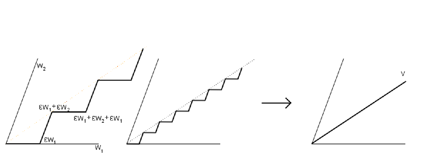
For a better understanding of the curves $\sigma_{\varepsilon}(t)$ and their limit, consider first the easier case when the $\gamma_{j}$ ’s were lines, $\gamma_{j}(t)=w_{j}t$ , and the $f_{p}$ ’s were translations, see Figure 1 above. In this case, the zig-zag curve is

\hat{\sigma}_{\varepsilon}(t):=\varepsilon w_{1}+\varepsilon w_{2}+\varepsilon w_{1}+\ldots+\bar{t}w_{i},

where $t=n\varepsilon+\bar{t}$ and $i=n\;({\rm mod}\;2)$ . In the sum there are $n+1$ terms. Thus,

\hat{\sigma}_{\varepsilon}(t)=\dfrac{n}{2}\varepsilon w_{1}+\dfrac{n}{2}\varepsilon w_{2}+o(\varepsilon)=\dfrac{t}{2}w_{1}+\dfrac{t}{2}w_{2}+o(\varepsilon)=tv+o(\varepsilon)

is $\varepsilon$ -close to the line $tv$ . Therefore, the curve $\hat{\sigma}(t):=\lim_{\varepsilon\to 0}\hat{\sigma}_{\varepsilon}(t)$ is such that

\dfrac{d\hat{\sigma}}{dt}(0)=v.

Define now another auxiliary curve. Let $f_{m}:=f_{\sigma_{\varepsilon}(m\varepsilon)}$ and $M_{m}$ be the matrix $(df_{m})_{0}$ . Set

\hat{\hat{\sigma}}_{\varepsilon}(t):=\varepsilon w_{1}+\varepsilon M_{1}w_{2}+\varepsilon M_{2}w_{1}+\ldots+\bar{t}M_{i}w_{i}.

By (3.1), there is a neighborhood $U$ of $0$ where $\left\|(df)_{0}-Id\right\|<\delta$ , for all $f\in\mathcal{F}$ with $f(0)\in U$ , and so $\left\|(df)_{0}\right\|<1+\delta$ , for all $f\in\mathcal{F}$ . Let $t^{*}>0$ such that

\sigma_{\varepsilon}(t),\hat{\sigma}_{\varepsilon}(t),\hat{\hat{\sigma}}_{\varepsilon}(t)\in U,\qquad\forall t\in[0,t^{*}].

Then we have

$\displaystyle\left\\|\hat{\sigma}_{\varepsilon}(t)-\hat{\hat{\sigma}}_{\varepsilon}(t)\right\\|$	$\displaystyle\leq$	$\displaystyle\sum_{i=1}^{n}\left\\|Id-M_{i}\right\\|\varepsilon\left\\|w_{i}\right\\|$
	$\displaystyle\leq$	$\displaystyle n\varepsilon\delta$
	$\displaystyle\leq$	$\displaystyle\frac{t}{\varepsilon}\varepsilon\delta$
	$\displaystyle=$	$\displaystyle t\delta.$

Also,

$\displaystyle\left\\|\sigma_{\varepsilon}(t)-\hat{\hat{\sigma}}_{\varepsilon}(t)\right\\|$	$\displaystyle=$	$\displaystyle\left\\|f_{n}(\gamma_{i}(\bar{t}))-\varepsilon w_{1}-\varepsilon M_{1}w_{2}-\varepsilon M_{2}w_{1}-\ldots-\bar{t}M_{i}w_{i}\right\\|$
	$\displaystyle\leq$	$\displaystyle\left\\|f_{n}(\gamma_{i}(\bar{t}))-(df_{n})_{0}\gamma_{i}(\bar{t})-f_{n}(0)\right\\|+\left\\|(df_{n})_{0}\gamma_{i}(\bar{t})-\bar{t}(df_{n})_{0}\dot{\gamma}_{i}(0)\right\\|$
		$\displaystyle\qquad\qquad+\left\\|f_{n-1}(\gamma_{i-1}(\bar{t}))-\varepsilon w_{1}-\varepsilon M_{1}w_{-}\ldots-\bar{t}M_{i-1}w_{i-1}\right\\|$
	$\displaystyle:=$	$\displaystyle I+II+III.$

Consider the last equation as the sum of three terms: $I$ , $II$ , and $III$ . Note that the first term can be bounded, cf. (3.2), by

I\leq\omega(\left\|\gamma_{i}(\bar{t})\right\|)\leq\omega(\varepsilon).

The second term is bounded by

II\leq\left\|(df_{n})_{0}\right\|\left\|\gamma_{i}(\bar{t})-\bar{t}\dot{\gamma}_{i}(0)\right\|\leq(1+\delta)\omega_{\gamma}(\varepsilon).

Finally, the third term is similar to the initial term: the right hand side in the calculation above, except that we have one term less. Therefore, we can iterate the procedure and get

	$\displaystyle\left\\|\sigma_{\varepsilon}(t)-\hat{\hat{\sigma}}_{\varepsilon}(t)\right\\|$	$\displaystyle\leq$	$\displaystyle n(\omega(\varepsilon)+(1+\delta)\omega_{\gamma}(\varepsilon))$
		$\displaystyle\leq$	$\displaystyle(t+1)\left(\dfrac{\omega(\varepsilon)}{\varepsilon}+(1+\delta)\dfrac{\omega_{\gamma}(\varepsilon)}{\varepsilon}\right).$

We are now ready to calculate the derivative at $0$ of $\sigma(t)$ . Indeed, for all $t\in U$ ,

$\displaystyle\left\\|\dfrac{\sigma(t)}{t}-v\right\\|$	$\displaystyle=$	$\displaystyle\lim_{\varepsilon\to 0}\left\\|\dfrac{\sigma_{\varepsilon}(t)}{t}-v\right\\|$
	$\displaystyle\leq$	$\displaystyle\lim_{\varepsilon\to 0}\left(\left\\|\dfrac{\hat{\sigma}_{\varepsilon}(t)}{t}-v\right\\|+\left\\|\dfrac{\hat{\sigma}_{\varepsilon}(t)-\hat{\hat{\sigma}}_{\varepsilon}(t)}{t}\right\\|+\left\\|\dfrac{\hat{\hat{\sigma}}_{\varepsilon}(t)-\sigma_{\varepsilon}(t)}{t}\right\\|\right)$
	$\displaystyle\leq$	$\displaystyle 0+\dfrac{t\delta}{t}+\lim_{\varepsilon\to 0}\dfrac{t+1}{t}\left(\dfrac{\omega(\varepsilon)}{\varepsilon}+(1+\delta)\dfrac{\omega_{\gamma}(\varepsilon)}{\varepsilon}\right)$
	$\displaystyle=$	$\displaystyle\delta.$

So, for $t\to 0$ , since $\delta$ is arbitrarily small, we have $\dfrac{d\sigma}{dt}(0)=v.$ So $v\in\Delta_{0}$ , i.e., $\Delta_{0}$ is a vector space.

From the transitive action of biLipschitz maps we have that $\Delta$ is invariant under $\mathcal{F}$ , so the dimension of $\Delta_{p}$ is constant.

The class $\Gamma$ is defined to be the curves $\{f_{p}\circ\sigma^{(v)}\}$ for $p$ in a neighborhood of the origin and $v\in\Delta_{0}$ . Such curves satisfy inequality (4.3) for a suitable $\omega_{\Gamma}$ since it is true for the $\gamma_{j}$ ’s that are in a finite number, then for the zig-zag limits and finally for all curves in $\Gamma$ , using that (3.2) implies that the $f$ ’s have a controlled distortion. For a similar reason, the curves in $\Gamma$ have uniform bound on the speed, i.e., (4.2) holds. ∎

From the previous lemma we have that, for each $p\in N$ , the set $\Delta_{p}$ is a $k$ -dimensional plane. So the map $p\mapsto(p,\Delta_{p})$ is a (not necessarily continuous) section of the grassmannian bundle. In the next subsection we will prove that this map is $C^{1}$ and so $\Delta$ is a $C^{1}$ sub-bundle.

We have noticed, more than once, that the $d$ -geodesics in our setting are Lipschitz curves with respect to the Euclidean metric, therefore they are absolutely continuous functions, i.e., they are differentiable almost everywhere and each curve is the integral of its derivative that is a priori just an $L^{1}$ function. On the other hand, each absolutely continuous curve can be reparametrized to be Lipschitz with respect to the Euclidean metric.

Definition 4.2.

Fixing a distribution $\Delta$ , a curve is called horizontal if it is absolutely continuous and it derivative lies in the distribution $\Delta$ wherever it exists.

We can now consider another distance on $N$ . In the literature, this distance has many different names: Carnot-Carathéodory metric, Sub-Riemannian metric, geometric control metric, nonholonomic mechanical metric.

(4.5)

d_{CC}(p,q)=\inf\left\{{\rm Length}_{\left\|\cdot\right\|}(\sigma)\;|\;\sigma\;{\rm horizontal\;from}\;p\;{\rm to}\;q\right\},

where ${\rm Length}_{\left\|\cdot\right\|}$ denotes the length with respect to the Euclidean metric.

4.1. Continuity of the sub-bundle

To prove that the sub-bundle $\Delta$ is in fact a $C^{1}$ sub-bundle, we will use a result that give a characterization of $C^{1}$ sub-manifold as ambiently $C^{1}$ -homogeneous compacta.

A set $A\subset\mathbb{R}^{n}$ is said to be ambiently $C^{1}$ -homogeneous if for every pair of points $x,y\in A$ , there exist neighborhoods $O_{x}$ and $O_{y}$ in $\mathbb{R}^{n}$ and a $C^{1}$ diffeomorphism

h:(O_{x},O_{x}\cap A,x)\to(O_{y},O_{y}\cap A,y).

Theorem 4.3 ([RSŠ96]).

Let $A\subset\mathbb{R}^{n}$ be compact. Then $A$ is ambiently $C^{1}$ -homogeneous if and only if $A$ is a $C^{1}$ submanifold of $\mathbb{R}^{n}$ .

The original proof of this result in [RSŠ96] requires the Rademacher Theorem. Shchepin and Repovš [SR00] simplify the proof by eliminating the need to invoke Rademacher.

Clearly, since the statement of Theorem 4.3 is local, then the assumption of compactness can be replaced by local compactness.

Proposition 4.4.

Let $\Delta\subset TN$ be a (not necessarily continuous) distribution. Suppose $\mathcal{F}=\{f_{p}\}_{p\in N}$ is a transitive family of local $C^{1}$ diffeomorphisms of $N$ , $f_{p}(0)=p$ , that leaves invariant $\Delta$ , i.e., $(df)(\Delta)=\Delta$ for any $f\in\mathcal{F}$ . If the map $p\mapsto(df_{p})_{0}$ is continuous at $p=0$ , then $\Delta$ is a continuous sub-bundle. If moreover there is another transitive family of $C^{2}$ diffeomorphisms that leaves invariant $\Delta$ , then $\Delta$ is a $C^{1}$ sub-bundle of the tangent bundle.

Proof.

The continuity of $\Delta$ at the origin is consequence of the continuity of $p\mapsto(df_{p})_{0}$ . Then continuity everywhere follows from the invariance under the transitive family of $C^{1}$ diffeomorphisms.

Let us denote by $h(p):=\Delta_{p}$ the $k$ -dimensional plane as an element in the $k$ -dimensional grassmannian ${\rm Gr}_{k}(T_{p}N)$ . We want to prove that $h$ is a $C^{1}$ function. Consider the map

\sigma:p\mapsto(p,h(p)),

i.e., the induced section of the grassmannian bundle ${\rm Gr}_{k}(TN)$ .

First notice that, since we proved that $\Delta$ is continuous, then $h$ is continuous. Being $\sigma$ the graph of the continuous function $h$ , then the image $M:=\sigma(N)$ is closed in ${\rm Gr}_{k}(TN)$ . Now, if $f$ is $C^{2}$ , then its differential $df$ induces a $C^{1}$ map $f_{*}$ of ${\rm Gr}_{k}(TN)$ . Moreover if a family of $C^{2}$ diffeomorphisms acts transitively on $N$ preserving $\Delta$ , then the induced maps on the grassmannian bundle act transitively on $M$ preserving $M$ . Thus, we use Theorem 4.3: since $M$ is a closed, so locally compact, subset of the manifold ${\rm Gr}_{k}(TN)$ that is ambiently $C^{1}$ -homogeneous, then $M$ is a $C^{1}$ sub-manifold of ${\rm Gr}_{k}(TN)$ .

Let $V\subseteq N$ be a neighborhood that trivialize the bundle

{\rm Gr}_{k}(TV)=V\times\mathbb{R}^{m}.

Call $\pi:V\times\mathbb{R}^{m}\to V$ the projection on the first space. Let $M^{\prime}:=M\cap(V\times\mathbb{R}^{m})$ . Since $M$ is a $C^{1}$ manifold, then

\rho:=\pi_{*}|_{TM^{\prime}}:TM^{\prime}\to TV

is a bundle map. Now, in the case that there exists a point $x\in M^{\prime}$ such that

(4.6)

\rho_{x}(T_{x}M^{\prime})=TN,

then, by the Implicit Function Theorem, in a neighborhood $U$ of $x$ , there is a $C^{1}$ function $\tilde{h}:U\to\mathbb{R}^{m}$ such that, locally,

\left\{(p,\tilde{h}(p))\;:\>p\in U\right\}=M=\left\{(p,h(p))\;:\>p\in U\right\}.

Thus $h=\tilde{h}$ and so $h$ is $C^{1}$ on the neighborhood $U$ . Using again that $M$ is $C^{1}$ -homogeneous, we have that each point in $M$ has a neighborhood on which $h$ is $C^{1}$ .

If (4.6) is not true for any $x\in M$ , we will get to a contradiction. Indeed, in this case

\dim(\ker\rho_{x})>0,\qquad\forall x\in M.

One then can find an open set $A\subset M$ such that $\dim(\ker\rho_{a})=c$ , for all $a\in A$ , for some constant $c>0$ . From general theory of sub-bundles [Ati67], we have that $\ker\rho\subset TA\subset TM$ is a sub-bundle of $TA\subset TM$ over $A\subset M$ . From this we have that locally there is a non-trivial section $X:A\to\ker\rho$ . In other words, $X$ is a vector field on $A$ such that $X_{a}\in\ker(\pi_{*}|_{T_{a}A})$ , for all $a\in A$ . This means that $X_{a}$ is of the form $(0,X^{(2)}_{a})\in TM\times T\mathbb{R}^{m}$ . If now $\gamma$ is an integral curve for $X$ , then we may assume that $\gamma$ is not constant since $X$ is non-trivial. However,

\gamma(t)=\gamma(0)+\int_{0}^{t}X_{\gamma(t)}dt=\gamma(0)+\left(0,\int_{0}^{t}X^{(2)}_{\gamma(t)}dt\right).

But this contradicts the fact that $M$ is a graph. ∎

5. Proof of biLipschitz equivalence

In the previous section we used the fact that the $d$ -rectifiable curves are differentiable almost everywhere, by Proposition 3.3, to construct a distribution $\Delta$ coming from the derivatives of such curves. Now, with the next result, we conclude the proof of Theorem 2.1.

Theorem 5.1.

Let $(N,d)$ satisfy the assumptions of Theorem 2.1. Let $\Delta$ be the distribution defined above in (4.1). Let $d_{CC}$ be any Carnot-Carathéodory metric associated to $\Delta$ . Then we have, locally,

\frac{1}{L}d_{CC}(p,q)\leq d(p,q)\leq Ld_{CC}(p,q),

for some $L>0$ .

Proof.

We need to prove two inequalities.

5.1. The first inequality

This is straightforward. Given $p\in N$ , let $\gamma_{p}$ be a $d$ -geodesic from $0$ to $p$ . Since by Proposition 3.3 the $d$ distance is greater than the Euclidean distance, $\gamma_{p}$ is Lipschitz, thus it is differentiable almost everywhere. We may parametrize $\gamma_{p}$ by arc length with respect to $d$ , so $\gamma_{p}:[0,T]\to N$ , where $T:=d(0,p)$ . We claim that $\left\|\dot{\gamma}_{p}\right\|(t)\leq 1$ , for almost every $t$ . Indeed, for any point $t$ of differentiability,

\left\|\dot{\gamma}_{p}(t)\right\|=\lim_{h\to 0}\dfrac{\left\|\gamma_{p}(t+h)-\gamma_{p}(t)\right\|}{h}\leq\lim_{h\to 0}\dfrac{d(\gamma_{p}(t+h),\gamma_{p}(t))}{h}=\dfrac{h}{h}=1.

d_{CC}(p,0)\leq{\rm Length}_{\left\|\cdot\right\|}(\gamma_{p})=\int_{0}^{T}\left\|\dot{\gamma}_{p}(t)\right\|dt\leq\int_{0}^{T}1dt=T=d(0,p).

5.2. The second inequality

Given a point $p\in N$ , we want to construct a $d$ -rectifiable curve $\sigma$ that starts at $0$ and ends arbitrarily close to $p$ , whose $d$ -length is close to the $CC$ -distance of $p$ from $0$ . This will be enough since the metric $d$ gives the standard topology. To construct such a curve, we will use the curves of the family $\Gamma$ defined in Lemma 4.1. For any $v\in\Delta$ there is a pre-chosen curve $\gamma_{v}\in\Gamma$ such that $\dot{\gamma}_{v}(0)=v$ , and these curves have a common bound for the speed (4.2) and for the distance from the linear approximation (4.3).

Take any $\eta:[0,T]\to\mathbb{R}^{n}$ that is a Lipschitz curve, almost everywhere tangent to the distribution $\Delta$ , with $\eta(0)=0$ , $\eta(T)=p$ , i.e., one of the candidate curves in the calculation of the CC-distance between $0$ and $p$ . We can suppose that $\eta$ is parametrized by arc length, i.e., $\left\|\dot{\eta}\right\|=1$ , so $T={\rm Length}_{\left\|\cdot\right\|}(\eta)$ . Our goal is to show that $T$ is greater than a fixed constant times $d(0,p)$ .

Recall that $\Delta$ is $C^{1}$ . Thus, in a neighborhood of $0$ , that we will still call $N$ , we can find a $C^{1}$ framing $\{X_{1},\ldots,X_{k}\}$ of $\Delta$ , i.e., each $X_{j}$ is a $C^{1}$ vector field and

\Delta_{p}={\rm Span}\{(X_{1})_{p},\ldots,(X_{k})_{p}\},\quad\forall p\in N.

We may assume that $\{(X_{1})_{p},\ldots,(X_{k})_{p}\}$ is an orthonormal basis of $\Delta_{p}$ . Since $N$ is compact, for some $C>0$ , each vector field $X_{j}$ is $C$ -Lipschitz, i.e.,

\left\|(X_{j})_{q_{1}}-(X_{j})_{q_{2}}\right\|\leq C\left\|q_{1}-q_{2}\right\|,\quad\forall q_{1},q_{2}\in N.

A consequence is that if $v\in\Delta_{q_{1}}$ is such that $\left\|v\right\|\leq 1$ then there is $w\in\Delta_{q_{2}}$ with $\left\|w\right\|\leq 1$ such that $\left\|v-w\right\|\leq C\left\|q_{1}-q_{2}\right\|.$ Indeed, since $\{(X_{j})_{q_{1}}\}$ is an orthonormal basis, there are numbers $a_{j}$ such that $v=\sum_{j}a_{j}(X_{j})_{q_{1}}$ with $\sum_{j}|a_{j}|\leq 1.$ Thus $w:=\sum_{j}a_{j}(X_{j})_{q_{2}}$ satisfies

|v-w|\leq\sum_{j}|a_{j}|\left\|(X_{j})_{q_{1}}-(X_{j})_{q_{2}}\right\|\leq C\left\|q_{1}-q_{2}\right\|.

What we conclude is that each $v\in\Delta_{q_{1}}$ with $\left\|v\right\|\leq 1$ has distance less than $C\left\|q_{1}-q_{2}\right\|$ from the unit ball in $\Delta_{q_{2}}$ . Denoting by $U(\Delta_{q})$ the unit ball in $\Delta_{q}$ , we write

(5.1)

{\rm dist}(U(\Delta_{q_{2}}),U(\Delta_{q_{2}}))\leq C\left\|q_{1}-q_{2}\right\|

5.2.1. The construction of $\sigma$ .

Take $\varepsilon>0$ . Construct piece-by-piece a curve $\sigma$ in the following way. Start at $0=\eta(0)$ . After a suitable choice of a vector $v_{0}\in\Delta_{0}$ , we will take the curve $\gamma_{v_{0}}(t)\in\Gamma$ , where $\Gamma$ is the fixed family of curves from Lemma 4.1, and then we will define the first piece of $\sigma(t)$ as, for $0\leq t\leq\varepsilon$ ,

(5.2)

\sigma(t):=\gamma_{v_{0}}(t).

By (5.1), since $\left\|\dot{\eta}(t)\right\|\leq 1$ for a.e. $t$ , we have that, for a.e. $t\leq\varepsilon$ ,

{\rm dist}(U(\Delta_{0}),\dot{\eta}(t))\leq C\left\|\eta(t)\right\|\leq C|t|\leq C\varepsilon,

since $\eta$ is parametrized by arc length. Since the unit ball $U(\Delta_{0})$ is convex, we have

{\rm dist}\left(U(\Delta_{0}),\frac{1}{\varepsilon}\int_{0}^{\varepsilon}\dot{\eta}(t)dt\right)\leq C\varepsilon.

Therefore there exists a $v_{0}\in\Delta_{0}$ with $\left\|v_{0}\right\|\leq 1$ such that

(5.3)

\left\|v_{0}-\frac{1}{\varepsilon}\int_{0}^{\varepsilon}\dot{\eta}(t)dt\right\|\leq C\varepsilon.

So for $0\leq t\leq\varepsilon$ , the curve $\sigma$ has been defined by (5.2).

For the inductive construction of $\sigma$ suppose that for any $t\leq n\varepsilon$ , the value $\sigma(t)$ has been defined. We shall define $\sigma$ as, for $n\varepsilon<t\leq(n+1)\varepsilon$ ,

\sigma(t):=\gamma_{v_{n}}(t-n\varepsilon),

for a suitable choice of $v_{n}\in\Delta_{\sigma(n\varepsilon)}$ and its related $\gamma_{v_{n}}\in\Gamma$ .

First note that $\lim_{t\to n\varepsilon^{+}}\sigma(t)=\gamma_{v_{n}}(n\varepsilon-n\varepsilon)=\gamma_{v_{n}}(0)=\sigma(n\varepsilon)$ . Therefore the new piece agrees with the previous one, i.e., the path is continuous. Moreover, $\sigma((n+1)\varepsilon)=\gamma_{v_{n}}(\varepsilon).$ Then calculate the (right)-derivative at $n\varepsilon$ :

\left.\frac{d}{dt}\sigma(t)\right|_{t=n\varepsilon^{+}}=\dot{\gamma}_{v_{n}}(n\varepsilon-n\varepsilon)=\dot{\gamma}_{v_{n}}(0)=v_{n}.

Again using (5.1), we have that there exists $w_{n}\in\Delta_{\eta(n\varepsilon)}$ with $\left\|w_{n}\right\|\leq 1$ such that

\left\|w_{n}-\frac{1}{\varepsilon}\int_{n\varepsilon}^{(n+1)\varepsilon}\dot{\eta}(t)dt\right\|\leq C\varepsilon.

Also, since

{\rm dist}(U(\Delta_{\sigma(n\varepsilon)}),w_{n})\leq C\left\|\sigma(n\varepsilon)-\eta(n\varepsilon)\right\|,

there exists a vector $v_{n}\in\Delta_{\sigma(n\varepsilon)}$ with $\left\|v_{n}\right\|\leq 1$ such that

\left\|w_{n}-v_{n}\right\|\leq C\left\|\sigma(n\varepsilon)-\eta(n\varepsilon)\right\|.

(5.4)

\left\|v_{n}-\frac{1}{\varepsilon}\int_{n\varepsilon}^{(n+1)\varepsilon}\dot{\eta}(t)dt\right\|\leq C\left\|\sigma(n\varepsilon)-\eta(n\varepsilon)\right\|+C\varepsilon.

Let us now estimate $\left\|\eta(T)-\sigma(T)\right\|$ . We will show that we have a system of the following type:

(5.5)

\left\{\begin{array}[]{ccl}\left\|\eta(\varepsilon)-\sigma(\varepsilon)\right\|&\leq&o(\varepsilon)\\ \left\|\eta(n\varepsilon)-\sigma(n\varepsilon)\right\|&\leq&(1+C\varepsilon)\left\|\eta((n+1)\varepsilon)-\sigma((n+1)\varepsilon)\right\|+o(\varepsilon),\quad\forall n\in\mathbb{N},\end{array}\right.

where $\dfrac{o(\varepsilon)}{\varepsilon}\to 0$ , as $\varepsilon\to 0$ . Observe that a sequence of the form

(5.6)

\left\{\begin{array}[]{cl}a_{1}=&\alpha\\ a_{n}=&\beta a_{n-1}+\alpha\end{array}\right.

has solution $a_{n}=\alpha(\beta^{n-1}+\ldots+1)=\alpha\dfrac{1-\beta^{n}}{1-\beta}.$ So, from (5.5),

$\displaystyle\left\\|\eta(T)-\sigma(T)\right\\|$	$\displaystyle=$	$\displaystyle\left\\|\eta\left(\frac{T}{\varepsilon}\varepsilon\right)-\sigma\left(\frac{T}{\varepsilon}\varepsilon\right)\right\\|$
	$\displaystyle\leq$	$\displaystyle o(\varepsilon)\dfrac{1-(1-\varepsilon C)^{\frac{T}{\varepsilon}}}{1-(1-\varepsilon C)}$
	$\displaystyle\simeq$	$\displaystyle\dfrac{o(\varepsilon)}{\varepsilon}(1-e^{CT})\longrightarrow 0,\qquad{\rm as}\;\varepsilon\to 0.$

One big triangular inequality

Now, let us do the calculation showing (5.5). The case $n=1$ is shown by considering the following four curves and comparing them at time $t=\varepsilon$ :

(1)

$\eta(t)$ ,
(2)

$t\frac{1}{\varepsilon}\int_{0}^{\varepsilon}\dot{\eta}(s)ds$
(3)

$tv_{0}$ ,
(4)

$\sigma(t)=\gamma_{v_{0}}(t)$ .

Step by step,

1 and 2:

At time $\varepsilon$ , the curves are at the same point, by the Fundamental Theorem of Calculus.

2 and 3:

By (5.3), we have

\left\|\varepsilon v_{0}-\varepsilon\frac{1}{\varepsilon}\int_{0}^{\varepsilon}\dot{\eta}(t)dt\right\|\leq C\varepsilon^{2}.

3 and 4:

Since $\gamma\in\Gamma$ , by (4.3) we have $\left\|\varepsilon v_{0}-\gamma_{v_{0}}(\varepsilon)\right\|<\omega_{\Gamma}(\left\|v_{0}\right\|\varepsilon)<\omega_{\Gamma}(\varepsilon)$ .

Thus putting everything all together with the triangle inequality:

\left\|\eta(\varepsilon)-\sigma(\varepsilon)\right\|\leq C\varepsilon^{2}+\omega_{\Gamma}(\varepsilon).

For $n>1$ , more estimates are needed. We compare the following five curves at time $t=(n+1)\varepsilon$ :

(1)

$\eta(t)$ ,
(2)

$(t-n\varepsilon)\frac{1}{\varepsilon}\int_{n\varepsilon}^{(n+1)\varepsilon}\dot{\eta}(t)dt+\eta(n\varepsilon)$ ,
(3)

$(t-n\varepsilon)\frac{1}{\varepsilon}\int_{n\varepsilon}^{(n+1)\varepsilon}\dot{\eta}(t)dt+\sigma(n\varepsilon)$ ,
(4)

$(t-n\varepsilon)v_{n}+\sigma(n\varepsilon)$ ,
(5)

$\sigma(t)=\gamma_{v_{n}}(t-n\varepsilon)$ .

Step by step,

1 and 2:

At time $(n+1)\varepsilon$ , as before, the curves are at the same point:

\eta((n+1)\varepsilon)=\eta(n\varepsilon)+\varepsilon\frac{1}{\varepsilon}\int_{n\varepsilon}^{(n+1)\varepsilon}\dot{\eta}(t)dt.

2 and 3:

One is just a translations of the other by $\left\|\eta(n\varepsilon)-\sigma(n\varepsilon)\right\|.$

3 and 4:

As before, by (5.4),

\left\|\varepsilon v_{n}-\varepsilon\frac{1}{\varepsilon}\int_{n\varepsilon}^{(n+1)\varepsilon}\dot{\eta}(t)dt\right\|\leq C\varepsilon\left\|\sigma(n\varepsilon)-\eta(n\varepsilon)\right\|+C\varepsilon^{2}.

4 and 5:

From (4.3), the distance between the fourth and fifth curve is

$\displaystyle\left\\|\varepsilon v_{n}+\sigma(n\varepsilon)-\gamma_{v_{n}}(\varepsilon)\right\\|$	$\displaystyle=$	$\displaystyle\left\\|\varepsilon\dot{\gamma}_{v_{n}}(0)+\gamma_{v_{n}}(0)-\gamma_{v_{n}}(\varepsilon)\right\\|$
	$\displaystyle\leq$	$\displaystyle\omega_{\Gamma}(\left\\|v_{n}\right\\|\varepsilon)$
	$\displaystyle\leq$	$\displaystyle\omega_{\Gamma}(\varepsilon).$

Thus, putting everything together with the triangle inequality:

	$\displaystyle\left\\|\eta((n+1)\varepsilon)-\sigma((n+1)\varepsilon)\right\\|$	$\displaystyle\leq$	$\displaystyle C\varepsilon^{2}+\left\\|\eta(n\varepsilon)-\sigma(n\varepsilon)\right\\|+\varepsilon C\left\\|\sigma(n\varepsilon)-\eta(n\varepsilon)\right\\|+\omega_{\Gamma}(\varepsilon)$
		$\displaystyle\leq$	$\displaystyle(1+\varepsilon C)\left\\|\eta(n\varepsilon)-\sigma(n\varepsilon)\right\\|+C\varepsilon^{2}+\omega_{\Gamma}(\varepsilon).$

Thus, with the terminology of the system (5.6), $\beta=1+\varepsilon C$ and $\alpha=C\varepsilon^{2}+\omega_{\Gamma}(\varepsilon)=o(\varepsilon).$ Then, as we observed after (5.6), $\left\|\eta(T)-\sigma(T)\right\|\to 0$ , as $\varepsilon\to 0$ . This show that we can choose $\varepsilon$ to have $\sigma(T)$ as close as we want to $\eta(T)$ .

Now we calculate $d(0,\sigma(T))$ :

$\displaystyle d(0,\sigma(T))$	$\displaystyle\leq$	$\displaystyle\sum_{n<T/\varepsilon}d(\sigma(n\varepsilon),\sigma((n+1)\varepsilon))$
	$\displaystyle=$	$\displaystyle\sum d(\gamma_{v_{n}}(0),\gamma_{v_{n}}(\varepsilon))$
	$\displaystyle\leq$	$\displaystyle\sum_{1}^{T/\varepsilon}S\left\\|v_{n}\right\\|\varepsilon$
	$\displaystyle\leq$	$\displaystyle\sum_{1}^{T/\varepsilon}S\varepsilon=S\varepsilon\dfrac{T}{\varepsilon}=ST$
	$\displaystyle=$	$\displaystyle S{\rm Length}_{\left\\|\cdot\right\\|}(\eta),$

where we used, in order, the triangle inequality, then the definition of $\sigma$ , i.e., the fact that $\gamma_{v_{n}}(t)=\sigma(n\varepsilon+t)$ , then that $\gamma_{v_{n}}$ is $d$ -rectifiable parametrized by (uniformly) bounded speed, i.e., (4.2) holds, then the bound for $\left\|v_{n}\right\|$ . ∎

6. The case of biLipschitz maps coming from a Lie group action

We now describe how Theorem 1.1 can be proved using Theorem 2.1. What we need to show is that the properties of the transitive action can be improved, i.e., steps 1 and 2 of the outlined argument in the introduction can be done. Let $G$ , $H$ , and $d$ be as in Theorem 1.1.

6.1. Getting a closed and embedded subgroup of Homeo(G/H)

Any element of $G$ induces a diffeomorphism of $G/H$ . Without loss of generality, we can assume that $G$ acts effectively, so that it may be viewed as a subgroup of ${\rm Diff}(G/H)$ : the space of all $C^{\infty}$ -diffeomorphisms of $G/H$ equipped with the $C^{\infty}$ topology given by uniform convergence on compact sets of the functions together with all of their derivatives. So $G$ has two different natural topologies: the first one as a subset of ${\rm Diff}(G/H)$ and the second one (weaker) as a subset of ${\rm Homeo}(G/H)$ : the space of all homeomorphisms of $G/H$ equipped with the $C^{0}$ -topology, i.e., uniform convergence on compact sets. The first topology is more helpful since it gives control on the derivatives, however, the second one is easier to control by category arguments.

The following proposition tells us that we may assume that the inclusion $\iota:G\hookrightarrow{\rm Homeo}(G/H)$ is an embedding and that $\iota(G)$ is closed. In other words, for any sequence of elements of $G$ , viewed as a sequence of maps on $G/H$ , that converges uniformly on compact sets, the limit map is still an element of $\iota(G)$ , and the convergence is, in fact, as elements of $G$ , and so the sequence converges as maps in ${\rm Diff}(G/H)$ .

In general a Lie group $G$ acting on $G/H$ can fail to have the above property. Here is an example. Let $G$ be the group of isometries of $\mathbb{R}^{4}$ generated by the translations and a non-closed $1$ -parameter subgroup of $O(4)$ . So $G$ is a connected Lie group of dimension $5$ , acting on $\mathbb{R}^{4}$ . Thus, to have a group that is closed in ${\rm Homeo}(R^{4})$ , one has to extend the group to a bigger group, in this case the closure of $G$ in Isom $(G)$ . What is not trivial in general is that such larger group can be chosen to be still a Lie group.

Proposition 6.1.

Let $G$ be a Lie group and $H$ be a closed subgroup. Then there exists a Lie group $\hat{G}$ that extends the action of $G$ on $G/H$ and is embedded in ${\rm Homeo}(G/H)$ as a closed set. (Moreover, $G/H=\hat{G}/\hat{H}$ , for some closed subgroup $\hat{H}$ .)

The rest of this subsection is devoted to the proof of Proposition 6.1. Let $X$ be the homogeneous space $G/H$ . After taking the quotient of $G$ by the kernel of the action, we can suppose $G$ acts effectively on $X$ . Then we can replace $G$ by its universal cover, so it is a simply connected Lie group acting on $X$ effectively in a neighborhood of the identity $e\in G$ .

Let $V$ denote the subspace of vector fields on $X$ that corresponds to the Lie algebra of $G$ . In other words, for each $\xi\in L(G):=T_{e}G$ , the one-parameter subgroup of $G$

t\longmapsto\exp(t\xi)\in G

acts on $X$ by translation. So, for any $x\in X$ and $t\in\mathbb{R}$ , we can consider the flow on $X$

\Phi_{\xi}(t,x):=\exp(t\xi)\cdot x.

Differentiating, we obtain a vector field on $X$ that gives the above flow: for $x\in X$ ,

(6.1)

\xi(x):=d(\exp(t\xi)\cdot x)_{t=0}\in T_{x}X.

Abusing terminology the vector field is still called $\xi$ since we can identify $V$ and $L(G)$ . Indeed, $V$ is isomorphic to $L(G)$ as vector spaces (and even the bracket operation, up to sign, is preserved, as shown in [Hel01]). In particular, we point out that there is also a one-to-one correspondence of the above flows with elements in $V$ (or $L(G)$ ). Indeed,

(6.2)

\Phi_{\xi}(t,\cdot)=\Phi_{\xi^{\prime}}(t,\cdot)\in{\rm Homeo}(X),\,\forall t\in\mathbb{R}\quad\Longrightarrow\quad\xi=\xi^{\prime}\in V,

because of the local effectivity of the action: for $t$ small enough, $\exp(t\xi)\cdot x=\exp(t\xi^{\prime})\cdot x\in G/H$ implies $\exp(t\xi)=\exp(t\xi^{\prime})\in G$ and then $t\xi=t\xi^{\prime}\in L(G)$ since $\exp$ is a local diffeomorphism at the origin in $L(G)$ .

The vectors in the Lie algebra of $H$ correspond to those vector fields in $V$ that vanish at the origin $[e]\in X$ ,

(6.3)	$\displaystyle\xi\in L(H)$	$\displaystyle\Longleftrightarrow$	$\displaystyle\exp(t\xi)\in H,\quad\forall t\in\mathbb{R}$
		$\displaystyle\Longleftrightarrow$	$\displaystyle\exp(t\xi)[e]=[e],\quad\forall t\in\mathbb{R}$
		$\displaystyle\Longleftrightarrow$	$\displaystyle\Phi_{\xi}(t,[e])=[e],\quad\forall t\in\mathbb{R}$
		$\displaystyle\Longleftrightarrow$	$\displaystyle\xi([e])=0.$

Note that if $g\in G$ , then the translation $\tau_{g}:X\longrightarrow X$ , induced by the left translation, $xH\mapsto gxH$ , preserves the vector fields in $V$ ; this is just another manifestation of the adjoint representation¹¹ 1 The map $h\mapsto g^{-1}hg$ is differentiable and fixes the origin. Its differential at the origin is a homomorphism of the Lie algebra called ${\rm Ad}_{g}$ . The map $\displaystyle G$ $\displaystyle\longrightarrow$ $\displaystyle GL(T_{e}G)$ $\displaystyle g$ $\displaystyle\mapsto$ $\displaystyle{\rm Ad}_{g}$ is a representation of $G$ inside the algebra homomorphisms of the Lie algebra. of $G$ : we have the formula $g\exp(\xi)g^{-1}=\exp({\rm Ad}_{g}\xi)$ , see [Kna02, page 53], so ${\rm Ad}_{g}\xi\in L(G)$ is the push-forward vector field. However, we shall be interested in the fact that $\tau_{g}$ preserves the flows of vector fields in $V$ ; indeed, we get $g\exp(t\xi)=\exp(t{\rm Ad}_{g}\xi)g$ and so

(6.4)

\tau_{g}(\Phi_{\xi}(t,x)))=\Phi_{{\rm Ad}_{g}\xi}(t,\tau_{g}(x)).

The new group $\hat{G}$ extending the action of $G$ will come from the set of homeomorphisms of $X$ , that, as the elements of $G$ in (6.4), preserve the flows of vector fields in $V$ .

If $\{g_{k}\}\subseteq G$ is a sequence that converges as maps in ${\rm Homeo}(X)$ uniformly on compact sets to a homeomorphism $f:X\longrightarrow X$ , then we claim that $f$ also preserves $V$ , in the sense that for any $\xi\in V$ the flow $\Phi_{\xi}(t,x)$ is conjugated by $f$ to the flow $\Phi_{\xi^{\prime}}(t,x)$ for some $\xi^{\prime}\in V,$ i.e., for any $t\in\mathbb{R}$ , the diagram

\begin{array}[]{cclc}\Phi_{\xi}(t,\cdot):&X&\longrightarrow&X\\ &f\downarrow&&\quad\downarrow f\\ \Phi_{\xi^{\prime}}(t,\cdot):&X&\longrightarrow&X\end{array}

commutes. Since, because of (6.4), any $g\in G$ preserves $V$ , the claim is a consequence of the more general lemma:

Lemma 6.2.

The space of homeomorphisms preserving $V$ is $C^{0}$ -closed.

Proof.

Let $\{g_{k}\}_{k\in N}$ be a sequence of homeomorphisms (not necessarily coming from the $G$ action) preserving $V$ , i.e., for any $\xi\in V$ and any $k$ there exists a $\xi_{k}\in V$ such that the following diagram commutes:

\begin{array}[]{cclc}\Phi_{\xi}(t,\cdot):&X&\longrightarrow&X\\ &g_{k}\downarrow&&\quad\downarrow g_{k}\\ \Phi_{\xi_{k}}(t,\cdot):&X&\longrightarrow&X\end{array}.

If $g_{k}\to f$ in Homeo $(X)$ , then the above diagram (for fixed $\xi$ and $t$ ), converges uniformly on compact sets to

\begin{array}[]{cclc}\Phi_{\xi}(t,\cdot):&X&\longrightarrow&X\\ &f\downarrow&&\quad\downarrow f\\ \Phi_{\infty}(t,\cdot):&X&\longrightarrow&X\end{array}.

Recall that $L(G)$ is finite dimensional, so, after passing to a subsequence, either $\xi_{k}$ converges in direction, i.e., the sequence of unit vectors $\frac{\xi_{k}}{||\xi_{k}||}$ converges to some $v_{1}$ or is zero for all $k$ . In the second case, there is nothing else to prove since, for any $k$ , $g_{k}$ is the identity, and so is the limit. In the first case, we can complete $v_{1}$ to a basis $v_{1},\ldots,v_{n}$ of $L(G)$ . Defining $T_{k}:=\left\|\xi_{k}\right\|$ , write $\xi_{k}=T_{k}\sum_{j=1}^{n}a_{kj}v_{j}$ so, for $j=2,\ldots n$ , $a_{kj}\longrightarrow 0$ and $a_{k1}\longrightarrow 1$ , as $k\to\infty$ .

Note that $\Phi_{\xi}(0,\cdot)={\rm Id}$ , and so $\Phi_{\infty}(0,\cdot)={\rm Id}$ . Pick $p\in X$ . Since $\Phi_{\infty}$ is continuous in $t$ , for any $\varepsilon>0$ , there exists $\delta$ such that

{\rm Diam}\left(\Phi_{\infty}([0,\delta],p)\right)<\varepsilon.

We denoted by Diam the diameter of a set with respect to some fixed metric on $X$ inducing the same topology. Now, by uniform convergence, for any $\varepsilon>0$ , there exists $K\in\mathbb{N}$ such that, for any $k>K$ ,

\Phi_{\xi_{k}}([0,\delta],p)\subset{\rm Nbhd}_{\varepsilon}\left(\Phi_{\infty}([0,\delta],p)\right).

Therefore,

(6.5)

\Phi_{\xi_{k}}([0,\delta],p)\subset{\rm Nbhd}_{2\varepsilon}(p).

We may assume that $p$ is not a fixed point of the vector field $v_{1}$ . Take a time $t>0$ such that $q:=\Phi_{v_{1}}(t,p)\neq p$ . Suppose we chose $\varepsilon<|p-q|/3$ . Assume by contradiction that $T_{k}\to\infty$ . Take $k$ big enough such that $\dfrac{t}{T_{k}}<\delta$ . Since, for $s_{k}=\dfrac{t}{T_{k}}$ very small,

$\displaystyle\Phi_{\xi_{k}}(s_{k},p)$	$\displaystyle=$	$\displaystyle\Phi_{T_{k}\sum_{j=1}^{n}a_{kj}v_{j}}(s_{k},p)$
	$\displaystyle=$	$\displaystyle\Phi_{\sum_{j=1}^{n}a_{kj}v_{j}}(T_{k}s_{k},p)$
	$\displaystyle=$	$\displaystyle\Phi_{\sum_{j=1}^{n}a_{kj}v_{j}}(t,p)\longrightarrow\Phi_{v_{1}}(t,p)=q.$

But this contradicts (6.5), which says that, for all $k$ , the points $\Phi_{\xi_{k}}(s_{k},p)$ lie in a neighborhood of $p$ and so outside the ball $B(q,\frac{\epsilon}{3})$ , for how we have chosen $\varepsilon$ , and therefore they cannot converge to $q$ .

From the contradiction we deduce that the sequence $\xi_{k}$ is bounded so, after passing to a subsequence, it converges to some $\xi^{\prime}$ and $\Phi_{\infty}$ has to be the flow of $\xi^{\prime}$ (by uniqueness of limit). In particular $\xi^{\prime}$ is uniquely determined by $\Phi_{\infty}$ , by (6.2). We proved that every subsequence has a convergent sub-subsequence, and the limit is independent of the choice of the subsequence; therefore $\xi_{k}$ actually converges to a fixed $\xi^{\prime}\in V$ , giving the conclusion of the lemma. ∎

By (6.2), the vector field $\xi^{\prime}$ of the lemma is uniquely determined by $\Phi_{\infty}$ and so by $f$ and $\xi$ . Therefore we have a well-defined function $f_{*}:V\rightarrow V$ , such that

f(\Phi_{\xi}(t,x)))=\Phi_{f_{*}\xi}(t,f(x)).

Note that this induced map on the space $V$ is functorial, i.e., $f_{*}\circ g_{*}=(f\circ g)_{*}$ for any such maps $f$ and $g$ . If $g$ is an element in $G$ , then $g_{*}={\rm Ad}_{g}$ , so $g_{*}$ is a Lie algebra homomorphisms of $V$ . Now, suppose that $g_{k}\in{\rm Homeo}(X)$ have the similar property that the maps $\xi\mapsto(g_{k})_{*}\xi$ are Lie algebra homomorphisms of $V$ . Then if $g_{k}\to f$ in ${\rm Homeo}(X)$ , the map $\xi\mapsto f_{*}\xi$ is also a Lie algebra homomorphism of $V$ , because $f_{*}\xi=\lim_{k\to\infty}(g_{k})_{*}\xi$ . In other words, fixing a base for $L(G)$ , the maps $(g_{k})_{*}$ are square matrices converging pointwise to a square matrix $f_{*}$ .

Moreover, if the origin $[e]\in X$ is preserved by $f$ , then $f_{*}$ preserves $L(H)$ , i.e.,

(6.6)

f([e])=[e]\quad\Longrightarrow\quad f_{*}(L(H))=L(H);

the reason is just the characterization (6.3): $\xi\in L(H)$ if and only if $\xi([e])=0$ if and only if, for every $t\in\mathbb{R}$ , $[e]=f([e])=f(\Phi_{\xi}(t,[e]))=\Phi_{f_{*}\xi}(t,f([e]))=\Phi_{f_{*}\xi}(t,[e])$ if and only if $f_{*}\xi([e])=0$ if and only if $f_{*}\xi\in L(H)$ .

We can consider the group Homeo_V of homeomorphisms that preserve $V$ , in the sense of the lemma above and induce a Lie algebra homomorphism on $V$ .

Definition 6.3 ( ${\rm Homeo}_{V}$ ).

The set ${\rm Homeo}_{V}$ is the group of homeomorphisms $f\in{\rm Homeo}(X)$ such that there exists a Lie algebra homomorphism $f_{*}:L(G)\to L(G)$ with the property $f(\Phi_{\xi}(t,x)))=\Phi_{f_{*}\xi}(t,f(x))$ , or, explicitly, for all $t\in\mathbb{R}$ , $\xi\in V$ , and $x\in X$ ,

(6.7)

f(\exp(t\xi)x)=\exp(tf_{*}\xi)f(x).

Lemma 6.2 just says that the closure of $G$ in Homeo $(X)$ is contained in Homeo_V, and, more generally, Homeo_V is closed in Homeo $(X)$ .

Lemma 6.4.

The group ${\rm Homeo}_{V}$ is generated by left translations by elements of $G$ and automorphisms of $G$ that fix $H$ . In particular, any element $f\in{\rm Homeo}_{V}$ can be written uniquely as the composition of a translation and such an automorphism, in fact, if $[g]=f([e])$ , with $g\in G$ , then

(6.8)

f=\tau_{g}\circ\hat{\Lambda}_{{\rm Ad}^{-1}_{g}\circ f_{*}},

where $\tau_{g}$ is the translation by $g$ and $\hat{\Lambda}_{{\rm Ad}^{-1}_{g}\circ f_{*}}$ is the map induced on the quotient by the (unique) group automorphism of $G$ with differential ${\rm Ad}^{-1}_{g}\circ f_{*}$ .

Proof.

We first argue that if a map $f\in{\rm Homeo}_{V}$ fixes $[e]$ and $f_{*}={\rm Id}_{V}$ then in fact $f={\rm id}_{X}$ . Indeed, we claim that the set of fixed points $F:=\{gH\in G/H\,:\,f(gH)=gH\}$ is non-empty, closed and open, and so it is all of $G/H$ , i.e., the function $f$ is the identity. Indeed, $F$ is non-empty since the class of the identity is in it by assumption and it is closed since it is defined by a closed relation. The fact that $F$ is open is a consequence of $\exp$ being locally invertible. Indeed, take any $g^{\prime}$ that is close enough to $g\in F$ so that it can be written as $g^{\prime}=\exp(\xi)g$ for some $\xi\in L(G)$ . Then

f(g^{\prime}H)=f(\exp(\xi)gH)=\exp(f_{*}\xi)f(gH)=\exp(\xi)gH=g^{\prime}H.

It is a classical fact, [Kna02, page 49], that since $G$ is simply connected, for any (Lie algebra) homomorphism $\psi$ of $L(G)$ , there exists a unique smooth (group) homomorphism $\Lambda_{\psi}$ of $G$ such that $(d\Lambda_{\psi})_{e}=\psi$ . Moreover, in our setting, when $\Lambda_{\psi}$ is $H$ -invariant (so it passes to the quotient $X=G/H$ ), then $\Lambda_{\psi}\in{\rm Homeo}_{V}$ and we point out that $(\Lambda_{\psi})_{*}=\psi$ . Indeed, since $\Lambda_{\psi}$ is a homomorphism,

\Lambda_{\psi}(\exp(t\xi)x)=\Lambda_{\psi}(\exp(t\xi))\Lambda_{\psi}(x)=\exp(t\psi\xi)f(x).

Suppose now that $f:X\to X$ is any map belonging to ${\rm Homeo}_{V}$ . Take $g\in G$ such that that $[g]=f([e])$ and pre-compose $f$ by the translation $\tau^{-1}_{g}$ , so that $(\tau^{-1}_{g}\circ f)([e])=[e]$ . Take the automorphism $\Lambda:G\to G$ whose induced automorphism $V\to V$ is the inverse of $(\tau_{g}^{-1}\circ f)_{*}$ . Explicitly, we take $\Lambda=\Lambda_{((\tau^{-1}_{g})_{*}\circ f_{*})^{-1}}=\Lambda_{f_{*}^{-1}\circ{\rm Ad}_{g}}$ . Moreover, $\tau_{g}^{-1}\circ f$ fixes the origin and so $(\tau_{g}^{-1}\circ f)_{*}$ fixes $L(H)$ , and so $\Lambda$ fixes $H$ . Therefore, passing to the quotient $G/H$ , we have a homeomorphism $\hat{\Lambda}:X\to X$ . Then $\hat{\Lambda}\circ\tau_{g}^{-1}\circ f:X\to X$ fixes $[e]\in X$ and maps each left invariant vector field to itself, i.e., $(\hat{\Lambda}\circ\tau_{g}^{-1}\circ f)_{*}={\rm Id}$ . Hence, from what we showed at the beginning of the proof, $\hat{\Lambda}\circ\tau^{-1}_{g}\circ f$ is the identity, i.e., $f=\tau_{g}\circ\hat{\Lambda}^{-1}.$ The uniqueness comes from the fact that the intersection between translations and automorphisms is trivial. ∎

Lemma 6.5.

The group ${\rm Homeo}_{V}$ is a Lie group of diffeomorphisms and the inclusion ${\rm Homeo}_{V}\hookrightarrow{\rm Homeo}(X)$ is an embedding with closed image.

Proof.

The previous lemma says that every element of ${\rm Homeo}_{V}$ is a diffeomorphism. In fact, the lemma is claiming more: observe that the group of left translations and the group of automorphisms of $G$ fixing $H$ are both Lie groups; the first one is equivalent to $G$ itself, and the second one is a closed subgroup of Aut $(G)$ and Aut $(G)$ is a Lie group since automorphisms of a Lie group come from automorphisms of the Lie algebra, i.e., linear transformations of a finite dimensional vector space. Let $K_{1}$ be the group of left translations and $K_{2}$ be the group of automorphisms of $G$ fixing $H$ . The previous lemma says that as sets ${\rm Homeo}_{V}=K_{1}K_{2}.$ Note that $K_{1}$ is normal in ${\rm Homeo}_{V}$ . Indeed, for any $\tau_{g}\in K_{1}$ left translation by $g\in G$ and any $\phi\in K_{2}$ , we have

$\displaystyle(\phi^{-1}\circ\tau_{g}\circ\phi)(xH)$	$\displaystyle=$	$\displaystyle(\phi^{-1}\circ\tau_{g})(\phi(x)\phi(H))$
	$\displaystyle=$	$\displaystyle\phi^{-1}(g\phi(x)H)$
	$\displaystyle=$	$\displaystyle\phi^{-1}(g)(\phi^{-1}\circ\phi)(x)\phi^{-1}(H)$
	$\displaystyle=$	$\displaystyle\phi^{-1}(g)xH=\tau_{\phi^{-1}(g)}(xH).$

So $\phi^{-1}\circ\tau_{g}\circ\phi\in K_{1}$ . Thus, we have ${\rm Homeo}_{V}=K_{1}\rtimes K_{2}$ is a semi-direct product of Lie groups, so it is a Lie group.

Now, the fact that the inclusion has closed image is just Lemma 6.2. However, we must show that it is an embedding. This comes from the fact that $V$ is finite dimensional and every sequence of matrices converges $C^{\infty}$ as soon as it converges point-wise. Indeed, take $f_{k}\in{\rm Homeo}_{V}$ , we need to show that, under the hypothesis that $\{f_{k}\}_{k}$ converges in ${\rm Homeo}(X)$ , then it converges in ${\rm Homeo}_{V}$ . (Recall that ${\rm Homeo}(X)$ has the $C^{0}$ topology but ${\rm Homeo}_{V}$ has the $C^{\infty}$ one.) Since $f_{k}\in{\rm Homeo}_{V}$ , there are associated maps $(f_{k})_{*}\in GL(V)$ . The proof of Lemma 6.2 shows that for any $\xi\in V$ the sequence $(f_{k})_{*}\xi$ converges to $f_{*}\xi$ , where $f\in{\rm Homeo}_{V}$ is the $C^{0}$ -limit of $f_{k}$ . Since $\{(f_{k})_{*}\}_{k}$ are linear endomorphisms of the finite dimensional vector space $V$ that converge point-wise, then the convergence is in fact in $C^{\infty}(V)$ .

So, since by assumption we have , then in particular we have convergence at the point $[e]=H$ , i.e., , for some $g_{k}\in G$ . This means that there exist $h_{k}\in H$ such that . Call $g^{\prime}:=g_{k}h_{k}$ , so $[g_{k}^{\prime}]=[g_{k}]=f_{k}([e])$ , thus we can use the formula (6.8) and have

f_{k}=\tau_{g^{\prime}_{k}}\circ\Lambda_{{\rm Ad}^{-1}_{g^{\prime}_{k}}\circ f_{*}}.

Now, since , then and . From this last formula and from the fact that , we know that, defining $\hat{f}_{k}:=\tau_{g_{k}^{\prime}}^{-1}\circ f_{k}=\Lambda_{{\rm Ad}^{-1}_{g^{\prime}_{k}}\circ f_{*}}$ , we have that , and so that $\{f_{k}\}_{k}$ is converging in the $C^{\infty}$ topology. ∎

End of the proof of Proposition 6.1.

Consider the space $V$ of vector fields given by (6.1). Let $\hat{G}:={\rm Homeo}_{V}$ be the group as in Definition 6.3, of the homeomorphisms of the homogeneous space preserving $V$ in the sense of (6.7) and inducing homomorphisms on the algebra. Then from Lemma 6.5, we know that $\hat{G}$ extends the action of $G$ , consists of $C^{\infty}$ diffeomorphisms, is a Lie group and is a closed, embedded subgroup of ${\rm Homeo}(X)$ . ∎

Remark 6.6.

By Proposition 6.1, without loss of generality we may assume that $G$ has the following property: as soon as a sequence of elements $g_{n}\in G$ converges as maps of $X$ in the $C^{0}$ -topology, then the limit is a map coming from $G$ , the convergence is also in the topology of $G$ itself, and, moreover, since the action is smooth, the sequence also converges in the $C^{\infty}$ -topology.

6.2. Getting uniformly biLipschitz maps close to the identity

Remember that $G$ acts by diffeomorphisms on $G/H$ . Suppose now that, for any two points in a neighborhood of the identity, there is an element of $G$ , sending the first point to the second one, that is biLipschitz with respect to the geodesic metric $d$ . The following lemma tells us that, by staying enough close to the origin $[e]$ , we may assume that these elements of $G$ give maps that are uniformly biLipschitz and are $C^{\infty}$ -close to the identity as much as we want. Such argument is based on the Baire Category Theorem and has been used several times in the theory of homogenous compacta, e.g. in [MNP98, Theorem 3.1] or [Hoh85, Theorem 6.1].

Lemma 6.7.

Let $d$ be a metric on a homogeneous space $X=G/H$ inducing the usual topology. Suppose $G$ is closed and embedded in ${\rm Homeo}(G/H)$ . Let $U$ be a compact neighborhood of the origin $[e]\in G/H$ where the elements of $G$ that are biLipschitz with respect to the metric $d$ , act transitively. Then there exists a constant $k$ such that, for any $\varepsilon>0$ , there exists a smaller neighborhood $U_{\varepsilon}$ of the origin where the elements of $G$ that are $k$ -biLipschitz with respect to both a fixed Riemannian metric on $X$ and the metric $d$ and are $\varepsilon$ close to the identity with respect to a fixed $C^{\infty}$ distance, act transitively.

Proof.

The group $G$ can be seen as a subset of Diff $(G/H)$ . Since the action is smooth, the topology of $G$ is the same as that of any of those induced by any $C^{\infty}(G/H)$ -distance²² 2 We recall that $f_{n}$ converges to $f$ in $C^{\infty}(X)$ if, for any $p\in X$ , for any charts $\phi$ and $\psi$ at $p$ and $f(p)$ respectively, for any compact $K\subset\mathbb{R}^{n}$ inside the domain of $\phi$ , and any multi-index $\alpha\in\mathbb{N}^{n}$ , we have that the associated seminorm goes to zero, i.e., $\sup_{K}D^{\alpha}\left(\phi^{-1}\circ f_{n}\circ\phi-\phi^{-1}\circ f\circ\phi\right)\longrightarrow 0.$ In general, if $(\rho_{n})_{n\in N}$ is a sequence of seminorms defining a (locally convex) topological vector space $E$ , then $d(x,y)=\sum_{n=1}^{\infty}\frac{1}{2^{n}}\frac{\rho_{n}(x-y)}{1+\rho_{n}(x-y)}$ is a metric defining the same topology. . Fix one such distance and fix $\varepsilon>0$ . Consider a cover of $G$ by a countable number of closed balls $D_{n}$ for $n\in\mathbb{N}$ . We will say later how to choose the cover depending on $\varepsilon$ . So $G=\bigcup_{n\in\mathbb{N}}D_{n}$ with $D_{n}$ closed. Since any element of $G$ is smooth, then in particular it is locally biLipschitz with respect to any Riemannian metric on $X$ . Fix one such Riemannian metric. We will use the term $m$ -biLipschitz to describe to maps that are $m$ -biLipschitz for both the Riemannian metric and the metric $d$ , and the set of such maps will be denoted as ${\rm biLip}^{m}$ . Now consider the orbit set of $0$ in $U$ under $m$ -biLipschitz maps in $D_{n}$ , i.e.,

	$\displaystyle A_{n,m}$	$\displaystyle:=$	$\displaystyle(D_{n}\cap{\rm biLip}^{m})0$
		$\displaystyle:=$	$\displaystyle\left\{p\in U\;\|\;f(0)=p\;{\rm\;for\;some}\;m{\rm-biLipschitz\;map}\;f\;\in D_{n}\right\}.$

By transitivity, we have $U=\bigcup_{n\in\mathbb{N}}A_{n,m}.$ We claim that the $A_{n,m}$ are closed. Indeed, take $p_{j}\in A_{n,m}$ converging to $p\in U$ . Choose the $f_{j}\in D_{n}$ such that $f_{j}(0)=p_{j}.$ The $f_{j}$ ’s are $m$ -biLipschitz and $f_{j}(0)=p_{j}$ converges. The Ascoli-Arzelà argument implies that, after passing to a subsequence, $f_{j}$ converge to some $f$ , uniformly on compact sets and the limit function is $m$ -biLipschitz (for both metrics). Since $G$ is assumed to be closed in Homeo $(G/H)$ , then in fact $f\in G$ . From Remark 6.6, the convergence is in the $C^{\infty}$ topology, so, since $D_{n}$ is $C^{\infty}$ -closed, the limit function belongs to it and its value at $0$ is $p$ . Therefore, $f(0)=p$ for an $f\in D_{n}\cap{\rm biLip}^{m}$ . In other words, $p\in A_{n,m}$ , so $A_{n,m}$ is closed.

The Baire Category Theorem implies that one of the $A_{n,m}$ has non-empty interior. So there exists a compact $V\subset U$ , which is a neighborhood of some point $q$ , such that $V\subset A_{\bar{n},\bar{m}}$ for some $\bar{n},\bar{m}\in\mathbb{N}$ . Consider $f_{q}\in D_{\bar{n}}\cap{\rm biLip}^{\bar{m}}$ such that $f_{q}(0)=q$ .

We claim that we can take $U_{\varepsilon}:=f_{q}^{-1}(V)$ as our new neighborhood and $k:=\bar{m}^{4}$ as our required constant. Indeed, for any points $p_{1},p_{2}\in f_{q}^{-1}(V)$ , for $i=1,2$ , $f_{q}(p_{i})\in V\subset A_{\bar{n},\bar{m}}$ , so there exists $f_{i}\in D_{\bar{n}}\cap{\rm biLip}^{\bar{m}}$ such that $f_{i}(0)=f_{q}(p_{i})$ . Thus

p_{2}=\left(f_{q}^{-1}\circ f_{2}\circ f^{-1}_{1}\circ f_{q}\right)(p_{1})

and $f_{q}^{-1}\circ f_{2}\circ f^{-1}_{1}\circ f_{q}\in G$ is $k$ -biLipschitz. Moreover, $f_{q}^{-1}\circ f_{2}\circ f^{-1}_{1}\circ f_{q}$ is $\varepsilon$ close to the identity in Diff $(G/H)$ , if we had previously made a good choice of the cover $\{D_{n}\}$ , considering that the function $h\circ f\circ g^{-1}\circ h^{-1}$ is continuous in $f,g,h\in G$ .

Now we explain how to choose the cover, given $\varepsilon$ . Consider the map

\begin{array}[]{ccc}C^{\infty}(X)\times C^{\infty}(X)&\longrightarrow&C^{\infty}(X)\\ (g,h)&\longmapsto&g\circ h\circ g^{-1}.\end{array}

It is continuous and sends $C^{\infty}(X)\times\{{\rm id}\}$ to the identity function. Given a fixed $\varepsilon$ , there exists a neighborhood $V_{1}$ of the identity in $C^{\infty}(X)$ such that $C^{\infty}(X)\times V_{1}$ goes into the $\varepsilon$ -neighborhood of the identity function (the convergence is in $C^{\infty}(X)$ with respect to the $C^{\infty}$ -metric that we fixed). Now consider the map

\begin{array}[]{ccc}C^{\infty}(X)\times C^{\infty}(X)&\longrightarrow&C^{\infty}(X)\\ (g,h)&\longmapsto&g\circ h^{-1}.\end{array}

It is continuous and sends the diagonal $\Delta$ to the identity function. Given the neighborhood $V_{1}$ of before, there exists a neighborhood $V_{2}$ of $\Delta$ that is sent by the map into $V_{1}$ .

So if we had chosen the cover so that $D_{n}\times D_{n}\subset V_{2}$ for any $n\in\mathbb{N}$ , then, for any $f,g\in D_{n}$ , $f\circ g^{-1}\in V_{1}$ . Thus for any $h\in D_{n}$ , we have that $h\circ f\circ g^{-1}\circ h^{-1}$ lies in an $\varepsilon$ -neighborhood of the identity. This was what was left to prove. ∎

6.3. The end of the proof of Theorem 1.1 using Theorem 2.1

We can focus on a neighborhood $N$ of a point in the manifold that, after fixing a coordinate chart, is a neighborhood of $0$ in $\mathbb{R}^{n}$ . We can also transfer the geodesic metric imposing that the chart is an isometry. From now on we will identify the neighborhood in the manifold and that one in $\mathbb{R}^{n}$ .

We need to construct now a family of maps. The idea is to use Lemma 6.7 to select, for each $p$ in the neighborhood, a biLipschitz diffeomorphism $f_{p}$ whose differential $d(f_{p})$ differs from the identity by an error that depends only on $d(0,p)$ , and that tends to zero, as $d(0,p)$ tends to zero.

Considerthe neighborhoods $U_{1/n}$ given by Lemma 6.7, we can suppose that $N=U_{1}$ . Note that $\bigcap_{n}U_{1/n}=\{0\}$ . For $p=0$ , choose $f_{0}={\rm Id}$ ; for $p\in U_{1/n}\setminus U_{1/(n+1)}$ , Lemma 6.7 gives the existence of a $k$ -biLipschitz map $f_{p}$ so that $f_{p}(0)=p$ and which is $1/n$ close to the identity.

We need to show that the hypotheses of Theorem 2.1 apply. Since uniformly biLipschitz homogeneity is clear, we have left to show that condition (2.1) holds. It is satisfied, since in $N$ the second derivatives of the $f$ ’s are equibounded, say by $C$ , so

$\displaystyle\left\|\dfrac{\partial f_{i}}{\partial x_{j}}(x)-\dfrac{\partial f_{i}}{\partial x_{j}}(y)\right\|$	$\displaystyle\leq$	$\displaystyle\int_{0}^{\|x-y\|}\dfrac{d}{dt}\dfrac{\partial f_{i}}{\partial x_{j}}\left(x+t\frac{x-y}{\|x-y\|}\right)\,dt$
	$\displaystyle\leq$	$\displaystyle\int_{0}^{\|x-y\|}\sum_{k=1}^{n}\dfrac{\partial^{2}f_{i}}{\partial x_{k}\partial x_{j}}\left(x+t\frac{x-y}{\|x-y\|}\right)\frac{(x-y)_{k}}{\|x-y\|}\,dt$
	$\displaystyle\leq$	$\displaystyle nC\|x-y\|.$

Hence all of the hypotheses of Theorem 2.1 apply. Thus, there exists a sub-bundle $\Delta\subset TN$ , defined explicitly in (4.1), such that if $d_{\Delta}$ is any sub-Riemannian metric coming from $\Delta$ , then the geodesic metric $d$ is locally biLipschitz equivalent to $d_{\Delta}$ . The fact that $\Delta$ is invariant under the action of a transitive subset of a Lie group, will imply, by next proposition, that $\Delta$ is not just $C^{1}$ , but in fact smooth. ∎

Proposition 6.8.

Assume that $S$ is a set of elements of a Lie group $G$ that is transitive on the space $X:=G/H$ . Let $\Delta$ be a distribution on $X$ preserved by the action of $S$ . Then $\Delta$ must be real analytic.

Proof.

Since $S\subset G$ preserves the distribution $\Delta$ , then any product of its elements does. Call $G_{S}$ the group generated by $S$ . Consider $G_{1}:=\bar{G}_{S}$ the closure of $G_{S}$ in $G$ . The set $G_{1}$ is a Lie group and it preserves the distribution $\Delta$ too.

Fix a point $p\in X$ . Look at the orbit map of $p$ under $G_{1}$ ,

\Phi:G_{1}\longrightarrow X

g\mapsto g(p).

This is a smooth map, so we can take the derivative at the identity, i.e., the differential from the tangent space at the identity $L:=T_{e}G_{1}$ , the Lie algebra, and the tangent at $p$ , $T_{p}X$ ,

d\Phi_{e}:L\to T_{p}X.

Since this map is surjective, we can find a subspace $W$ of the Lie algebra of $G_{1}$ , such that the orbit map restricted to this subspace is an isomorphism of vector spaces,

d\Phi_{e}|_{W}:W\to T_{p}X.

Moreover, $\exp(W)$ is, locally, an analytic sub-variety. The orbit map $\Phi$ restricted to $\exp(W)$ gives an analytic map

\Phi|_{\exp(W)}:\exp(W)\to X.

By the Implicit Function Theorem, this is locally an analytic isomorphism.

From the hypothesis we know that, for any $g\in G_{1}$ , $\Delta_{g(p)}=g\Delta_{p}.$ Now, $g=\exp(v)$ , for some $v\in W$ , so we have the formula:

\Delta_{(\exp(v))(p)}=\exp(v)\Delta_{p}.

For any other point $q\in X$ , let $\Phi_{loc}^{-1}$ be a local inverse of $\Phi$ in a neighborhood of $q$ , so $q=\Phi(\exp(v))=(\exp(v))(p)$ and $\exp(v)=\Phi_{loc}^{-1}(q)$ . Then

\Delta_{q}=\Delta_{(\exp(v))(p)}=\exp(v)\Delta_{p}=\Phi_{loc}^{-1}(q)\Delta_{p}.

This implies that $\Delta$ is smooth because $\Delta_{q}$ depends analytically on $q$ . ∎

Appendix A Equality of piecewise $C^{1,1}$ and Lipschitz Carnot-Carathéodory metrics

One can define the Carnot-Carathéodory distance using as horizontal curves either Lipschitz curves tangent almost everywhere or piecewise $C^{1,1}$ curves, i.e., $C^{1}$ curves with Lipschitz derivative, tangent to the distribution. We prove now that piecewise $C^{1,1}$ horizontal curves or Lipschitz horizontal curves yield to the same Carnot-Carathéodory distances, when they both induce the manifold topology.

Theorem A.1.

Let $X$ be a Finsler manifold and let $\Delta$ be a locally Lipschitz sub-bundle of the tangent bundle. Let $d_{CC}^{C^{1,1}}$ and $d_{CC}^{Lip}$ be the Finsler-Carnot-Carathéodory metrics where the horizontal curves are chosen to be the class of curves that are, respectively, piecewise $C^{1,1}$ and Lipschitz, tangent to the distribution almost everywhere. Suppose that the two topologies induced by the two distances are the same as the topology of the manifold. Then the distances are the same, i.e., $d_{CC}^{C^{1,1}}=d_{CC}^{Lip}$ .

Proof. The fact that $d_{CC}^{C^{1,1}}\geq d_{CC}^{Lip}$ is obvious since all piecewise $C^{1,1}$ curves are Lipschitz. A priori, the infimum over all of the Lipschitz curve can be strictly smaller.

Since both metrics are path metrics, it suffices to prove the statement locally. So we may suppose that we are in $\mathbb{R}^{n}$ with a fixed norm $\left\|\cdot\right\|$ . In general, the space could be covered by small balls in which charts give a $(1+\varepsilon)$ -biLipschitz approximations. The $\varepsilon$ goes to zero as the diameters of the balls go to zero.

Take $\eta:[0,T]\to\mathbb{R}^{n}$ to be a Lipschitz curve, almost everywhere tangent to the distribution $\Delta$ , with $\eta(0)=0$ , $\eta(T)=p$ , i.e., one of the candidate to calculate the Lipschitz CC-distance between $0$ and $p$ . We can suppose that $\eta$ is parametrized by arclength, i.e., $\left\|\dot{\eta}\right\|=1$ a.e., so $T={\rm Length}(\eta)$ .

We will construct a sequence of piecewise $C^{1,1}$ curves whose length is smaller than or equal to the length of $\eta$ , going from $0$ to a sequence of points that converges to $p$ . Since the topologies are the same, this will give the conclusion.

Take $\varepsilon>0$ . Construct piece-by-piece a curve $\sigma$ in a way similar to that of Section 5.2. Start at $0=\eta(0)$ . After a suitable choice of a vector $v_{0}\in\Delta_{0}$ , we will take a curve $\gamma_{v_{0}}(t)$ , as the next Lemma A.2 says, and then we will define the first piece of $\sigma(t)$ as, for $0\leq t\leq\varepsilon$ ,

\sigma(t):=\gamma_{v_{0}}(t).

Each curve $\sigma$ that we will construct will have length less than $2T$ . On the Euclidean ball of radius $2T$ , the distribution $\Delta$ is $C$ -Lipschitz, for some $C>0$ . By the same discussion that in Section 5.2 led us to (5.1), we have that there exists $v_{0}\in\Delta_{0}$ with $\left\|v_{0}\right\|\leq 1$ such that

(A.1)

\left\|v_{0}-\frac{1}{\varepsilon}\int_{0}^{\varepsilon}\dot{\eta}(t)dt\right\|\leq C\varepsilon.

For the inductive construction of $\sigma$ suppose that for any $t\leq n\varepsilon$ , $\sigma(t)$ has been defined. We shall define $\sigma$ as, for $n\varepsilon<t\leq(n+1)\varepsilon$ ,

\sigma(t):=\gamma_{v_{n}}(t-n\varepsilon),

for a suitable choice of $v_{n}\in\Delta_{\sigma(n\varepsilon)}$ and its related $\gamma_{v_{n}}(t)$ given by Lemma A.2.

Take $w_{n}\in\Delta_{\eta(n\varepsilon)}$ with $\left\|w_{n}\right\|\leq 1$ such that

\left\|w_{n}-\frac{1}{\varepsilon}\int_{n\varepsilon}^{(n+1)\varepsilon}\dot{\eta}(t)dt\right\|\leq C\varepsilon.

Since $\Delta$ is $C$ -Lipschitz, there exists a vector $v_{n}\in\Delta_{\sigma(n\varepsilon)}$ with $\left\|v_{n}\right\|\leq 1$ such that

\left\|w_{n}-v_{n}\right\|\leq C\left\|\sigma(n\varepsilon)-\eta(n\varepsilon)\right\|.

(A.2)

\left\|v_{n}-\frac{1}{\varepsilon}\int_{n\varepsilon}^{(n+1)\varepsilon}\dot{\eta}(t)dt\right\|\leq C\left\|\sigma(n\varepsilon)-\eta(n\varepsilon)\right\|+C\varepsilon.

To estimate $\left\|\eta(T)-\sigma(T)\right\|$ , one uses system (5.5). The strategy of the proof for bounding the terms in system (5.5) is the same as that one in Section 5.2, except that instead of using (4.3), one uses Lemma A.2. Also, estimates (5.3) and (5.4) are replaced by (A.1) and (A.2).

The conclusion is that, as we observed after (5.6), $\left\|\eta(T)-\sigma(T)\right\|\to 0$ , as $\varepsilon\to 0$ . This shows that we can choose $\varepsilon$ to have $\sigma(T)$ as close as we want to $\eta(T)$ .

Now we calculate the length of $\sigma(0,T)$ :

$\displaystyle{\rm Length}(\sigma[0,T])$	$\displaystyle\leq$	$\displaystyle\sum_{n<T/\varepsilon}{\rm Length}(\sigma[n\varepsilon),\sigma((n+1)\varepsilon])$
	$\displaystyle=$	$\displaystyle\sum{\rm Length}(\gamma_{v_{n}}[0,\varepsilon])$
	$\displaystyle\leq$	$\displaystyle\sum_{1}^{T/\varepsilon}\left\\|v_{n}\right\\|\varepsilon$
	$\displaystyle\leq$	$\displaystyle\sum_{1}^{T/\varepsilon}\varepsilon=\varepsilon\dfrac{T}{\varepsilon}=T$
	$\displaystyle=$	$\displaystyle{\rm Length}(\eta[0,T]),$

where we used, in order, the triangle inequality, then the definition of $\sigma$ , then that $\gamma_{v_{n}}$ is parametrized by (uniformly) bounded speed, as Lemma A.2 says. ∎

Lemma A.2.

Given $v\in\Delta$ there exists a $C^{1,1}$ curve $\gamma_{v}$ starting at $v$ tangent to the distribution $\Delta$ , parametrized by speed smaller than $\left\|v\right\|$ and such that

\left\|\gamma_{v}(t)-[\gamma_{v}(0)+\dot{\gamma}_{v}(0)t]\right\|\leq Ct^{2}.

Proof.

Extend $v$ to a vector filed $X\subset\Delta$ using the orthogonal projection:

X_{p}:=\pi_{\Delta_{p}}(v).

The sub-bundle $\Delta$ is $C$ -Lipschitz, thus $X$ has the properties of being $C$ -Lipschitz, $v\in X$ and $\left\|X_{p}\right\|\leq\left\|v\right\|$ . Let $\gamma_{v}$ be the integral curve of $X$ starting at $v$ , i.e., $\dot{\gamma}_{v}(0)=v$ and $\dot{\gamma}_{v}(t)=X_{\gamma_{v}(t)}$ . Then

$\displaystyle{\rm Length}(\gamma_{v}[0,t])$	$\displaystyle=$	$\displaystyle\int_{0}^{t}\dot{\gamma}_{v}(s)ds$
	$\displaystyle\leq$	$\displaystyle\int_{0}^{t}\left\\|\dot{\gamma}_{v}(s)\right\\|ds$
	$\displaystyle=$	$\displaystyle\int_{0}^{t}\left\\|X_{\gamma_{v}(t)}\right\\|ds$
	$\displaystyle\leq$	$\displaystyle\int_{0}^{t}\left\\|v\right\\|ds\;=\;t\left\\|v\right\\|.$

In other words, $\gamma_{v}$ is of speed smaller than $\left\|v\right\|$ . The rest of the conclusion of the lemma is clear: since $X$ is $C$ -Lipschitz then it is differentiable a.e. with derivative bounded by $C$ . Thus $\gamma_{v}$ is a $C^{2}$ curve a.e. with second derivative bounded by $C$ . ∎

References

[AK00] Luigi Ambrosio and Bernd Kirchheim, Currents in metric spaces, Acta Math. 185 (2000), no. 1, 1–80.
[Ati67] Michael F. Atiyah, $K$ -theory, Lecture notes by D. W. Anderson, W. A. Benjamin, Inc., New York-Amsterdam, 1967.
[BBI01] Dmitriĭ Burago, Yuriĭ Burago, and Sergeiĭ Ivanov, A course in metric geometry, Graduate Studies in Mathematics, vol. 33, American Mathematical Society, Providence, RI, 2001.
[Bel96] André Bellaïche, The tangent space in sub-Riemannian geometry, Sub-Riemannian geometry, Progr. Math., vol. 144, Birkhäuser, Basel, 1996, pp. 1–78.
[Ber88] Valeriĭ N. Berestovskiĭ, Homogeneous manifolds with an intrinsic metric. I, Sibirsk. Mat. Zh. 29 (1988), no. 6, 17–29.
[Ber89a] by same author, Homogeneous manifolds with an intrinsic metric. II, Sibirsk. Mat. Zh. 30 (1989), no. 2, 14–28, 225.
[Ber89b] by same author, The structure of locally compact homogeneous spaces with an intrinsic metric, Sibirsk. Mat. Zh. 30 (1989), no. 1, 23–34.
[BGP92] Yuriĭ Burago, Mikhail Gromov, and Grigoriĭ Perel^′man, A. D. Aleksandrov spaces with curvatures bounded below, Uspekhi Mat. Nauk 47 (1992), no. 2(284), 3–51, 222.
[Bis01] Christopher J. Bishop, Bi-Lipschitz homogeneous curves in $\mathbb{R}^{2}$ are quasicircles, Trans. Amer. Math. Soc. 353 (2001), no. 7, 2655–2663 (electronic).
[BM91] Mladen Bestvina and Geoffrey Mess, The boundary of negatively curved groups, J. Amer. Math. Soc. 4 (1991), no. 3, 469–481.
[BP00] Marc Bourdon and Hervé Pajot, Rigidity of quasi-isometries for some hyperbolic buildings, Comment. Math. Helv. 75 (2000), no. 4, 701–736.
[CC97] Jeff Cheeger and Tobias H. Colding, On the structure of spaces with Ricci curvature bounded below. I, J. Differential Geom. 46 (1997), no. 3, 406–480.
[Che99] Jeff Cheeger, Differentiability of Lipschitz functions on metric measure spaces, Geom. Funct. Anal. 9 (1999), no. 3, 428–517.
[GH99] Manouchehr Ghamsari and David A. Herron, Bi-Lipschitz homogeneous Jordan curves, Trans. Amer. Math. Soc. 351 (1999), no. 8, 3197–3216.
[Gro96] Mikhael Gromov, Carnot-Carathéodory spaces seen from within, Sub-Riemannian geometry, Progr. Math., vol. 144, Birkhäuser, Basel, 1996, pp. 79–323.
[Gro99] Misha Gromov, Metric structures for Riemannian and non-Riemannian spaces, Progress in Mathematics, vol. 152, Birkhäuser Boston Inc., Boston, MA, 1999, Based on the 1981 French original [ MR0682063 (85e:53051)], With appendices by M. Katz, P. Pansu and S. Semmes, Translated from the French by Sean Michael Bates.
[GS92] Mikhail Gromov and Richard Schoen, Harmonic maps into singular spaces and $p$ -adic superrigidity for lattices in groups of rank one, Inst. Hautes Études Sci. Publ. Math. (1992), no. 76, 165–246.
[Hei01] Juha Heinonen, Lectures on analysis on metric spaces, Universitext, Springer-Verlag, New York, 2001.
[Hel01] Sigurdur Helgason, Differential geometry, Lie groups, and symmetric spaces, Graduate Studies in Mathematics, vol. 34, American Mathematical Society, Providence, RI, 2001, Corrected reprint of the 1978 original.
[HK98] Juha Heinonen and Pekka Koskela, Quasiconformal maps in metric spaces with controlled geometry, Acta Math. 181 (1998), no. 1, 1–61.
[Hoh85] Aarno Hohti, On Lipschitz homogeneity of the Hilbert cube, Trans. Amer. Math. Soc. 291 (1985), no. 1, 75–86.
[KB02] Ilya Kapovich and Nadia Benakli, Boundaries of hyperbolic groups, Combinatorial and geometric group theory (New York, 2000/Hoboken, NJ, 2001), Contemp. Math., vol. 296, Amer. Math. Soc., Providence, RI, 2002, pp. 39–93.
[KK05] Michael Kapovich and Bruce Kleiner, Coarse fibrations and a generalization of the Seifert fibered space conjecture, Manuscript (2005).
[KK06] by same author, Geometry of quasi-planes, Manuscript (2006).
[KL97] Bruce Kleiner and Bernhard Leeb, Rigidity of quasi-isometries for symmetric spaces and Euclidean buildings, Inst. Hautes Études Sci. Publ. Math. (1997), no. 86, 115–197 (1998).
[Kna02] Anthony W. Knapp, Lie groups beyond an introduction, second ed., Progress in Mathematics, vol. 140, Birkhäuser Boston Inc., Boston, MA, 2002.
[Laa02] Tomi J. Laakso, Plane with $A_{\infty}$ -weighted metric not bi-Lipschitz embeddable to ${\mathbb{R}}^{N}$ , Bull. London Math. Soc. 34 (2002), no. 6, 667–676.
[LP01] Urs Lang and Conrad Plaut, Bilipschitz embeddings of metric spaces into space forms, Geom. Dedicata 87 (2001), no. 1-3, 285–307.
[Mit85] John Mitchell, On Carnot-Carathéodory metrics, J. Differential Geom. 21 (1985), no. 1, 35–45.
[MM95] Gregori A. Margulis and George D. Mostow, The differential of a quasi-conformal mapping of a Carnot-Carathéodory space, Geom. Funct. Anal. 5 (1995), no. 2, 402–433.
[MNP98] Paul MacManus, Raimo Näkki, and Bruce Palka, Quasiconformally homogeneous compacta in the complex plane, Michigan Math. J. 45 (1998), no. 2, 227–241.
[Mon02] Richard Montgomery, A tour of subriemannian geometries, their geodesics and applications, Mathematical Surveys and Monographs, vol. 91, American Mathematical Society, Providence, RI, 2002.
[MZ74] Deane Montgomery and Leo Zippin, Topological transformation groups, Robert E. Krieger Publishing Co., Huntington, N.Y., 1974, Reprint of the 1955 original.
[Pan89] Pierre Pansu, Métriques de Carnot-Carathéodory et quasiisométries des espaces symétriques de rang un, Ann. of Math. (2) 129 (1989), no. 1, 1–60.
[RSŠ96] Dušan Repovš, Arkadij B. Skopenkov, and Evgenij V. Ščepin, $C^{1}$ -homogeneous compacta in ${\bf R}^{n}$ are $C^{1}$ -submanifolds of ${\bf R}^{n}$ , Proc. Amer. Math. Soc. 124 (1996), no. 4, 1219–1226.
[Sem96] Stephen Semmes, Good metric spaces without good parameterizations, Rev. Mat. Iberoamericana 12 (1996), no. 1, 187–275.
[SR00] Eugine V. Shchepin and Dušan Repovš, On smoothness of compacta, J. Math. Sci. (New York) 100 (2000), no. 6, 2716–2726, Pontryagin Conference, 2, Nonsmooth Analysis and Optimization (Moscow, 1998).

Hei01

$\displaystyle\|(df)_{0}(y)+f(0)-f(y)\|$	$\displaystyle\leq$	$\displaystyle\int_{0}^{1}\|(df)_{0}\cdot y-(df)_{ty}\cdot y\|\,dt$
	$\displaystyle\leq$	$\displaystyle\int_{0}^{1}\left\\|(df)_{0}-(df)_{ty}\right\\|\|y\|\,dt$
	$\displaystyle\leq$	$\displaystyle\int_{0}^{1}\eta(\|ty\|)\|y\|\,dt$
	$\displaystyle\leq$	$\displaystyle\int_{0}^{1}\eta(\|y\|)\|y\|\,dt$
	$\displaystyle=$	$\displaystyle\omega(\|{y}\|).$

	$\displaystyle\langle f_{j}(p)\|p\rangle$	$\displaystyle\geq$	$\displaystyle\langle p+p\|p\rangle-\left\\|f_{1}(p)-p-p\right\\|\cdot\left\\|p\right\\|$
		$\displaystyle\geq$	$\displaystyle 2\left\\|p\right\\|^{2}-\frac{1}{2}\left\\|p\right\\|^{2}\geq\frac{1}{2}\left\\|p\right\\|^{2}.$

$\displaystyle\langle f_{j+1}(p)\|p\rangle$	$\displaystyle\geq$	$\displaystyle\langle f_{j}(p)+p\|p\rangle-\left\\|f_{j+1}(p)-f_{j}(p)-p\right\\|\cdot\left\\|p\right\\|$
	$\displaystyle\geq$	$\displaystyle\langle f_{j}(p)\|p\rangle+\langle p\|p\rangle-\left\\|f_{j+1}(p)-f_{j+1}(0)-p\right\\|\cdot\left\\|p\right\\|$
	$\displaystyle\geq$	$\displaystyle\frac{j}{2}\left\\|p\right\\|^{2}+\left\\|p\right\\|^{2}-\frac{1}{2}\left\\|p\right\\|^{2}\geq\frac{j+1}{2}\left\\|p\right\\|^{2}.$

	$\displaystyle\left\\|\eta((n+1)\varepsilon)-\sigma((n+1)\varepsilon)\right\\|$	$\displaystyle\leq$	$\displaystyle C\varepsilon^{2}+\left\\|\eta(n\varepsilon)-\sigma(n\varepsilon)\right\\|+\varepsilon C\left\\|\sigma(n\varepsilon)-\eta(n\varepsilon)\right\\|+\omega_{\Gamma}(\varepsilon)$
		$\displaystyle\leq$	$\displaystyle(1+\varepsilon C)\left\\|\eta(n\varepsilon)-\sigma(n\varepsilon)\right\\|+C\varepsilon^{2}+\omega_{\Gamma}(\varepsilon).$

$\displaystyle\left\|\dfrac{\partial f_{i}}{\partial x_{j}}(x)-\dfrac{\partial f_{i}}{\partial x_{j}}(y)\right\|$	$\displaystyle\leq$	$\displaystyle\int_{0}^{\|x-y\|}\dfrac{d}{dt}\dfrac{\partial f_{i}}{\partial x_{j}}\left(x+t\frac{x-y}{\|x-y\|}\right)\,dt$
	$\displaystyle\leq$	$\displaystyle\int_{0}^{\|x-y\|}\sum_{k=1}^{n}\dfrac{\partial^{2}f_{i}}{\partial x_{k}\partial x_{j}}\left(x+t\frac{x-y}{\|x-y\|}\right)\frac{(x-y)_{k}}{\|x-y\|}\,dt$
	$\displaystyle\leq$	$\displaystyle nC\|x-y\|.$

Geodesic manifolds with a transitive subset of smooth biLipschitz maps

Abstract.

1. Introduction

Theorem 1.1.

Example: Affine maps giving homogeneity.

Theorem 1.2.

1.1. An outline of the proof of Theorem 1.1

1.2. Organization of the paper

Acknowledgements

2. The general criterion and some consequences

Theorem 2.1.

Theorem 2.2.

Proof.

Theorem 2.3.

Proof.

3. The given metric is greater than a Riemannian metric

Lemma 3.1.

Proof.

Lemma 3.2 (Uniform distortion control).

Proof.

Proposition 3.3.

Proof.

Remark 3.4.

4. The construction of the Carnot-Carathéodory metric

Lemma 4.1 (Control on curves Γ\Gamma representing Δ\Delta).

Proof.

Definition 4.2.

4.1. Continuity of the sub-bundle

Theorem 4.3 ([RSŠ96]).

Proposition 4.4.

Proof.

5. Proof of biLipschitz equivalence

Theorem 5.1.

Proof.

5.1. The first inequality

5.2. The second inequality

5.2.1. The construction of σ\sigma.

One big triangular inequality

6. The case of biLipschitz maps coming from a Lie group action

6.1. Getting a closed and embedded subgroup of Homeo(G/H)

Proposition 6.1.

Lemma 6.2.

Proof.

Definition 6.3 (HomeoV{\rm Homeo}_{V}).

Lemma 6.4.

Proof.

Lemma 6.5.

Proof.

End of the proof of Proposition 6.1.

Remark 6.6.

6.2. Getting uniformly biLipschitz maps close to the identity

Lemma 6.7.

Proof.

6.3. The end of the proof of Theorem 1.1 using Theorem 2.1

Proposition 6.8.

Proof.

Appendix A Equality of piecewise C1,1C^{1,1} and Lipschitz Carnot-Carathéodory metrics

Theorem A.1.

Lemma A.2.

Proof.

References

Lemma 4.1 (Control on curves $\Gamma$ representing $\Delta$ ).

5.2.1. The construction of $\sigma$ .

Definition 6.3 ( ${\rm Homeo}_{V}$ ).

Appendix A Equality of piecewise $C^{1,1}$ and Lipschitz Carnot-Carathéodory metrics