ITP-UU-08/17
SPIN-08/16
arXiv:yymm.nnnn
A LOCALLY FINITE MODEL FOR GRAVITY
Utrecht University
and
Spinoza Institute
Postbox 80.195
3508 TD Utrecht, the Netherlands
e-mail: g.thooft@phys.uu.nl
internet: http://www.phys.uu.nl/˜thooft/
Abstract
Matter interacting classically with gravity in 3+1 dimensions usually gives rise to a continuum of degrees of freedom, so that, in any attempt to quantize the theory, ultraviolet divergences are nearly inevitable. Here, we investigate matter of a form that only displays a finite number of degrees of freedom in compact sections of space-time. In finite domains, one has only exact, analytic solutions. This is achieved by limiting ourselves to straight pieces of string, surrounded by locally flat sections of space-time. Globally, however, the model is not finite, because solutions tend to generate infinite fractals. The model is not (yet) quantized, but could serve as an interesting setting for analytical approaches to classical general relativity, as well as a possible stepping stone for quantum models. Details of its properties are explained, but some problems remain unsolved, such as a complete description of the most violent interactions, which can become quite complex.
August 24, 2026
1 Introduction: Gravity in 2+1 dimensions
Classical point particles, interacting only gravitationally in 2+1 dimensions, require a limited number of physical degrees of freedom per particle.[1][2][3] Although they are surrounded by locally flat space-time (if the cosmological constant is taken to be zero), space-time may globally form a closed, compact universe.[4] The classical equations can be solved exactly, and for this reason this is a magnificent model for a complete, exactly solvable cosmology. Many researchers are more interested in quantized theories, where the point particles are removed as being unwanted topological defects, to be replaced by non-trivial global topological features of the universe. Such theories however have no local degrees of freedom at all, so from a conceptual point of view they are actually further removed from the physical world than our gravitating point particles.

Indeed, the importance of the model of gravitating point particles in a locally flat 2+1 dimensional space-time, is still severely underestimated. It will serve as a starting point for the 3+1 dimensional theory discussed in this paper. In 2+1 dimensions, pure gravity (gravity without matter in some small section of space-time) has no physical degrees of freedom at all. This is because the Riemann curvature can be rewritten in terms of a symmetric matrix as follows:
| (1.1) |
so that the Ricci curvature is
| (1.2) | |||
| (1.3) |
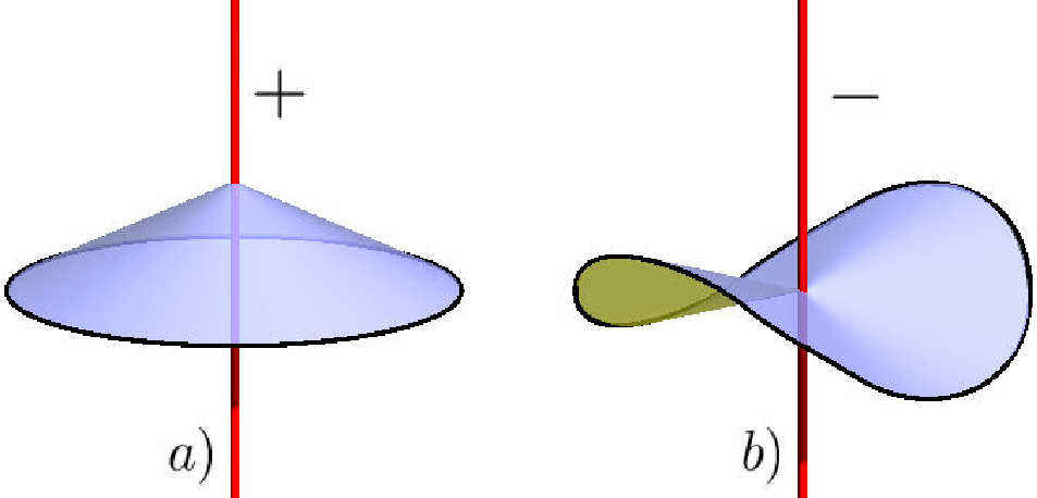
Clearly, if matter is absent, vanishes, and therefore so do and . Conversely, a point particle represents point curvature. Thus, particles are point singularities surrounded by flat space-time. A particle at rest can be described as in Figure 1. The wedge is stitched closed, so that the points and are identified. The defect angle can directly be identified with the particle’s rest mass. One can show that systems containing several point particles in motion, while the total momentum is kept zero, is surrounded by a conical space-time, of which the deficit angle can be identified with the total energy.11 1 There may however also be a time shift when a curve is followed around the cone. This time shift is then identified with total angular momentum. Only particles with negative rest mass, or systems with negative energy, are surrounded by a conical space-time with negative deficit angle, or surplus angle, see also Fig. 2.
When such a particle is set in motion, the surrounding space-time is described by performing Lorentz transformations upon the stationary case of Fig. 1. One then can study systems with many particles, by viewing space-time as a tessellation of locally flat triangles, or polygons. A number of surprises are encountered:
-
Using fast moving, heavy particles, a space-time can be created that appears to allow for the existence of closed timelike curves[5], much like in Gödel’s universe[6]. This would clash with fundamental principles of causality, but one can also show that in physically realistic models such configurations cannot occur, because a universe that contains such a “Gott pair” would actually collapse to a point before the timelike curve could be closed[7]. Any closed timelike curve that one would be tempted to construct would pass through a non-existing region of the universe.
-
If all particles in a 2 + 1 dimensional universe would be stationary or nearly stationary, the two-dimensional integrated scalar Ricci tensor, , would have to be positive, so with a sufficient number of particles the spacelike part of this universe would always close into an geometry. Its timelike coordinate can form a compact dimension (featuring both a bang and a crunch), or a semi-infinite one, with either a bang or a crunch.
-
With fast moving particles one can however also form 2-d surfaces with higher genus, without requiring negative mass particles.[8]
Quantization of this system is often carried out ‘as usual’,[9] but there are delicate problems, having to do with the fact that we are dealing with a strictly finite universe, so that the role of an ‘observer’ is questionable, and the statistical interpretation of the wave function is dubious because the finiteness of the universe prohibits infinite sequences of experiments to which a statistical analysis would apply. Carrying quantization out with care, one first observes that evidently, time is quantized into ‘Planck time’ units[10]. This is easily derived from the fact that the hamiltonian is an angle and it is bounded to the unit circle. Consequently, a quantum theory cannot be formulated using differential equations in time, but rather one should use evolution operators that bridge integral time segments. This indeed can be regarded as a first indication of some sort of space-time discreteness, which we will encounter later in a more concrete way. However, a confrontation with foundational aspects of quantum mechanics appears to be inevitable.
In this paper, the question is asked whether a similar “finite” theory can also be formulated in 3 + 1 dimensions. This is far from obvious. One first notices that the absence of matter now no longer guarantees local flatness, since the Ricci curvature can vanish without the total Riemann curvature being zero. However, one still can decide to view space-time as a tessellation of locally flat pieces. The defects in such a construction again may represent matter. The primary defects one finds are direct generalizations of the 2 + 1 dimensional case. Take a particle-like defect in 2-space. In 3+1 dimensions, such defects manifest themselves as strings.
Our starting point is that, indeed, straight strings are surrounded by a locally flat metric. In Section 2, we recapitulate the well-known derivation of the metric near such a string. Then, in Section 3, moving strings are described. These topics are quite elementary but we need these discussions to initiate the mathematical derivations that come next. In Section 4, joints between strings are introduced. Then we arrive at collisions. The orthogonal case (Section 5) seems to be the easiest case, though we will see that there is a catch, at the end. The most difficult case occurs when two strings approach at an angle. There are two possibilities. The “quadrangle” final state is discussed in Section 6. It leads to delicate mathematical relations between matrices. We needed to do some computer algebra, the result of which was deferred to the Appendix. This algebra reveals that, at the highest relative velocities of the approaching strings, the quadrangle final state is ruled out, so that more complex final states are expected. An attempt to describe these is made in Section 7.
2 Strings
It could be that matter is always arranged in such a way that it can be regarded as defects in a locally perfectly flat space-time. As opposed to technical approaches towards solving General Relativity[11], we now regard matter of this form as elementary. The novelty in this idea is that, in spite of matter being distributed on subspaces of measure zero, we still insist that it obeys local laws of causal behavior. Let us see how this looks.
By simply adding the third space dimension as a spectator, orthogonal to the first two, we find flat 3 dimensional space-time surrounding a string. Indeed, the energy momentum tensor of a straight, infinite, static string pointing in the -direction, is
| (2.1) |
where is the string tension parameter. When is small, the metric generated by such a string is found by slightly smearing the delta peak. The curvature is only in the transverse coordinates . Choosing conveniently scaled coordinates and replacing by
| (2.2) |
where , we find that for , the transverse components of the metric must be those of a sphere,
| (2.3) |
At , the transverse metric changes into that of a cone. The cone that touches the sphere at that point generates the metric
| (2.4) |
where the coordinate is matched to the coordinate at the point , . The deficit angle of the cone is .
Inside the smeared region, where the metric is that of Eq. (2.3), we have the Ricci curvature
| (2.5) |
while on the conical metric (2.4), the curvature vanishes. Substituting Eq. (2.1) into Einstein’s equation, one then gets
| (2.6) |
so that for small values of , the deficit angle can be written as
| (2.7) |
We quickly return to the old coordinates where the delta peak is very sharp. Space-time surrounding a string is then seen to be as sketched in Fig. 2. When the string constant is large, we redefine it to be the one generating exactly the deficit angle . Note that a positive string constant leads to a deficit angle. A negative string constant would produce a surplus angle, see Fig. 2. Normally, in string theory, a negative string constant would make a string highly unstable, as it contains positive pressure and negative energy. In our case, however, strings are constrained to form straight lines, and therefore this instability has no effect at small distances. We later may wish to include such negative strings in our models. We leave this open for the time being, but unless indicated specifically, we will usually be discussing strings with positive string constants and thus with positive deficit angles.
A more conventional derivation of the locally flat metric surrounding a string can be found for instance in [12].

3 Moving strings
A description of a multitude of static strings is now straightforward, in principle. However, already here, one may expect considerable complications. The system of static strings is not unlike the 2 + 1 dimensional universe with moving point particles, where the time coordinate is replaced by the coordinate of the static string system. We know that the 2 + 1 dimensional world has either a big bang singularity or a big crunch[4]. Similar “infrared” singularities might show up in the static string system. This question will not be further pursued here. It is the local properties of the model that we will investigate further.
Moving strings impose important questions concerning the internal consistency of the model. A moving string can be characterized in different ways. Firstly, one can specify the orientation vector of the string, normalized such that its norm coincides with half the deficit angle, when the string is at rest:
| (3.1) |
In addition then we specify the velocity vector of the string. But, noticing that the string is invariant under boosts in the direction , only the component of orthogonal to matters, so we limit ourselves to the case
| (3.2) |
Finally, the position of the string at should be specified. This requires another vector orthogonal to . All in all, this requires 3 + 2 + 2 = 7 real parameters, of which 5 are translationally invariant, and 2 can be set to zero by a spacelike translation in 3-space.
Alternatively, we can specify the string’s characteristics by giving the element of the Poincaré group that describes the holonomy along a non-contractible cycle around the string. For static strings through the origin of 3-space, this is just the pure rotation operator, which will be denoted as . For strings moving with velocity through the origin, this is the element of the Lorentz group, where is the element of that represents a pure Lorentz boost corresponding to the velocity .
If the string does not move through the origin, we get a more general element of the Poincaré group.
Notice however, that an arbitrary element of the Lorentz group is specified by 6 parameters, not 5, and the elements of the Poincaré group by 10 parameters, not 7. This means that not all elements of the Poincaré group describe the holonomy of a string. Firstly, ignoring the translational part, the pure Lorentz transformation associated to the closed curve has to obey one constraint:
There must be a Lorentz frame such that, in that frame, is a pure rotation in 3-space.
Since we plan to describe these Lorentz transformations in terms of their representations in , we identify this as a constraint on the associated matrices. Write
| (3.3) |
where are matrices representing boosts with velocity (we will see shortly that pure boosts are represented by hermitean matrices, Eq. (3.20)), and is a unitary matrix representing a pure rotation. When points in the direction, we have
| (3.4) |
so that
| (3.5) |
Since the trace is invariant under rotations and the boosts (3.3), it follows quite generally that
| (3.6) | |||||
| (3.7) |
Eq. (3.6) fixes one of the real variables of the Lorentz transformation . Inequality (3.7) is important in a different way. A generic matrix can de written in a basis where it is diagonal. Because the determinant is restricted to be 1, the diagonal form is then
| (3.8) |
where can be any complex number. Imposing (3.6) leaves two options: either is on the unit circle – in which case it represents a pure rotation in 3-space, or it is a positive or negative real number. In the latter case, is a pure Lorentz boost, and this is when Ineq. (3.7) is violated. It describes the holonomy of something that is quite different from a string. We return to that at the end of this section.
The second restriction to be imposed on the holonomy of a physical string is the translational part of the element of the Poincaré group. We just saw that in the frame where is diagonal, the string is static, and its position should be characterized by a vector orthogonal to . Using the same notation (3.3) to write the full Poincaré element , we add a displacement operator ( being the displacement vector):
| (3.9) |
where is the generator of the Lorentz transformation, and is the 4 dimensional displacement vector:
| (3.10) |
Henceforth, expressions such as stand short for a matrix acting on the 4-vector . In notation, this would read
| (3.11) |
where are the three Pauli matrices. From Eq. (3.9), we have
| (3.12) |
In the static case, , can neither have a time component nor a component parallel to . The time component could be introduced to describe a spinning string, analogous to a spinning point particle in dimensional gravity, but the problem with that is that such a space-time would possess closed timelike curves (CTC); thus, causality would be a problem.
A component of in the direction could be introduced as a generalization of the string concept; it would describe a string with torsion – one could call that a “spring”. We will not discuss springs further, but we have to keep this possibility in mind. Barring spin and torsion, gives two constraints on the vector .
Specifying the element of the Poincaré group that describes the holonomy associated to a non-contractible curve around a string, specifies its position provided does not vanish (vanishing strings have no specified position). To find the location of a string if is given is easy: just solve the equation
| (3.13) |
In the static case, this gives
| (3.14) |
where is the unit vector in the time direction, while and are free parameters. Thus, we find the string world sheet.
We end this section with a few important facts about Lorentz transformations in the representation, for future use.
- [1]
Pure rotations in 3-space are described by the subgroup of . Thus, is a pure rotation iff . We often write such a matrix as
(3.15) where
(3.16) and are the three Pauli matrices. is the rotation vector but with a different normalization:
(3.17) For a pure rotation along the -axis, see Eq. (3.4), and . Note that, as before (Eq. (3.1)), is half the full rotation angle.
- [2]
Pure Lorentz boosts are Hermitean matrices. Diagonalizing such a matrix corresponds to rotating into the -direction. The matrix then takes the form
(3.18) In general,
(3.19) where the vector is apart from a normalization:
(3.20) Notice that . Hermitean matrices with are equivalent to since all matrices describe the same Lorentz transformation as .
- [3]
Any Lorentz transformation can be associated to a vector and a vector such that it is the product of a pure boost and a pure rotation:
(3.21) Proof: define the matrix by
(3.22) and notice that, since is hermitean and positive definite, it can be written as
(3.23) where is also hermitian and, since , also . Diagonalizing gives us in diagonal form, and its eigenvalues (whose product is one), can be matched with the boost velocity which is again in the -direction in this frame. Finally, define as
(3.24) is unitary, therefore it describes a pure rotation in 3-space.
- [4]
Given any Lorentz transformation with , then there exists a pure boost operator and either a rotation or another pure boost such that
(3.25) Proof: looking at the eigenvalues of , one finds that, since their product is one and the sum is real, they either match the eigenvalues of or those of . A matrix that diagonalizes can be written as due to the previous theorem. So we have
(3.26) where stands for the matrix that is either a rotation or a boost. This rotation or boost was in the -direction, since was diagonal. The matrix rotates that vector into any other direction in 3-space.
We now return to Eqs. (3.13) and (3.14) for the string world sheet. Suppose we have a that obeys Eq. (3.6) but not the inequality (3.7). Then, in some Lorentz frame, this is a pure boost rather than a pure rotation. Write it as
| (3.27) |
where we took the boost to be in the -direction. The equation for the “world sheet”, , now leads to
| (3.28) |
in other words, the transverse plane at . This is a spacelike surface rather than a timelike string world sheet. What we find here is a “tachyonic” string. Such elements will be difficult to incorporate in a viable gravity model, if we wish to have some version of causality. We will therefore attempt to avoid structures for which the holonomy is a boost.
4 Connecting strings
We could try to limit ourselves to having only infinite, straight strings in our model, but as soon as collisions are considered – and we will argue that these are inevitable – one must face the presence of strings with finite lengths. These strings must then be connected to other strings in junctions, see Fig. 3. Just as our infinite strings, junctions are also surrounded by flat space [12]. The rules for connecting three strings , and are as follows.
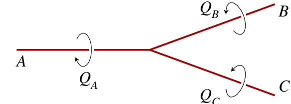
- )
The junction at time must lie on a point that is on the world sheet of the three strings and is a straight line. Thus, the three world sheets must have a straight line in 4-space in common. This line is a solution of
(4.1) (which is, again, in the 4 dimensional notation). Depending on whether this line is timelike, spacelike or lightlike, there are three classes of junctions: subluminal, superluminal and lightlike. Superluminal junctions will be seen to come in two types.
- )
The fact that the surrounding space-time is flat implies that the holonomies must match: or, if we take all strings pointing towards the junction (so that turns into its inverse),
(4.2)
In the case of a superluminal junction, the three strings have a spacelike line in common. This means that a special Lorentz frame exists where this is a straight line in the -direction that is instantaneous in time. The three connecting strings are parallel in that frame, but they may have different velocities. We either have one string splitting in two, or two strings merging into one. The first of these cases is impossible to reconcile with local causality, but the latter, in principle, is: two parallel strings meet and subsequently merge. Since the time reverse of this event violates causality, this would be an example of information loss. At first we will find that this kind of events may be difficult to avoid, but we will show how this can nevertheless be achieved if we so wish.
In more general Lorentz frames, superluminal junctions can be easily recognized as they describe a pair of strings opening up or closing like a superluminal zipper. A superluminal zipper that is opening up will have to be avoided at all times; the closing (joining) superluminal zipper is a curious case of information loss.
Lightlike and timelike (subluminal) junctions are fine.
If we wish two strings and to meet at one subluminal junction for an extended amount of time, then this gives three restrictions on the associated holonomies and alone: first, the product of their holonomies must again be a string holonomy, or
| (4.3) |
From this, one can show that in a Lorentz frame where string is static and pointing in the -direction, we have
| (4.4) |
where all coefficients are real. Our second restriction now is that, in Eq. (4.4),
| (4.5) |
which corresponds to a subluminal junction. If we have a superluminal junction. If the string is static as well. One easily checks that then is unitary and hence a pure rotation. The case for general positive is obtained by Lorentz boosting in the only allowed direction, the -direction (otherwise, would not remain static). Note that such a boost is described by Eq. (3.27).
Finally, of course, the displacement vectors of the Poincaré group elements must also match.
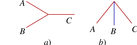
Thus, we will be specially interested in the case where, for every string junction, there exists a Lorentz frame where all three strings are static. If the string constants are large, so that the deficit angles (or possible surplus angles) are large, the situation is a bit complicated, since at a junction the three strings appear not to lie in a single plane. If the string constants ar weak, one discovers that, in principle, there are two types of subluminal junctions. They are sketched in Figure 4. In the first case, see Fig. 4, either all deficit angles are positive or they are all negative (i.e., all surplus angles are positive). This we will refer to as a regular junction. The strings behave as elastic bands connected at a point: each string appears to pull the two others towards it. In the case one string has a sign opposite to the two others, one gets the situation sketched in Fig. 4: it is the situation that can be deduced from the previous case by replacing the one string with the exceptional sign by an opposite-sign string pointing in the opposite direction.
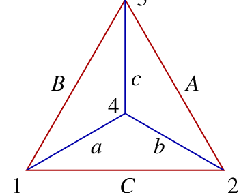
This information is useful if one wants to investigate whether constructions can be made with only finite extensions in space. Figure 5 shows an example of this. We have three strings, and forming a triangle, and three others, and that connect the three points to a point in the middle. The junctions 1, 2 and 3 are irregular because they contain only sharp angles. Clearly, the strings and must have signs opposite to the signs of and . Junction number 4 is a regular one.
In general, it is easy to argue that finite size constructions with only positive sign strings cannot be possible, since the entire thing is surrounded by flat space; hence there is no gravitational field; the total energy must be zero. This will not be possible with positive energy strings.
Much of the above remains true when the string constants, apart from their signs, are large, but things then are a bit more difficult to visualize, since space and space-time are locally but not globally flat.
In this paper we will not attempt to completely avoid the emergence of negative string constants. This would lead to negative energy states. One could think of addressing these at a later stage in a quantum theory by some kind of second quantization. As long as we restrict ourselves to local behavior this might not be a disaster, but of course the question of positive and negative string constants (deficit angles) will have to be addressed. We will advocate to avoid superluminal junctions of the splitting type at any stage, as these are difficult to reconcile with causality. Avoiding superluminal junctions of the joining type will be a bit harder, but we will finally find a procedure to avoid those together with the variety that opens up. Also all strings that violate the inequality (3.7) must be avoided since they too are impossible to reconcile with causality. These two demands will require so much of our attention that we will not further dwell on the signs of the string constants.
5 Orthogonal collisions
When we were dealing with point particles, in the 2 + 1 dimensional case, we could safely assume that the particles will never collide head-on. In general, they will miss one another, and consequently no further dynamical rules are needed to determine how an particle system will evolve. This will not be true in higher dimensional spaces22 2 Strings will in general not collide head-on in a space-time of more than 4 dimensions. However, the generalizations of the objects we discuss in this paper, in higher dimensions will be branes, not strings. Strings in 3 + 1 dimensional space-time will in general not be able to avoid one another. They will cross, and in doing so, two straight string sections will not be straight anymore after the collision.
Consider an initial state in which two strings are heading towards one another. We can always work in a Lorentz frame where one of the strings, call it , is at rest. The conical 3-space surrounding it has a deficit angle . In the generic case, in this Lorentz frame, the second string does not have to be oriented orthogonally to the first one. Its string constant, , does not have to be the same as . Consider now the velocity vector of the second string. If it is not orthogonal to the string , we perform a Lorentz boost in that direction. String will stay at rest. If is not orthogonal to the string , we replace it by one that is orthogonal to . This way, one convinces oneself that, in general, we can limit ourselves to the case where is orthogonal to both and .

However, it is a physical limitation if we also assume to be orthogonal to . Just because it is special, we consider this case first. The collision event is sketched in Fig. 6. In 6, the two strings approach one another. They both drag a space-time cusp with them. Now, what happens when hits , is best understood by drawing the cusp of in the opposite direction. The result of that, however, is that string is seen to have a kink. The same thing happens to string itself; it develops a kink due to the cusp of . After the passage, the two kinks must be connected by a new string, that stretches with and now moving away from one another.
Indeed, we see that, in general, the holonomy of string is non-trivial; it is obtained from the holonomies and of strings and as follows (depending on sign conventions for , and ):
| (5.1) |
and do not commute because they represent rotations along two different axes. Clearly, upon crossing, two strings produce a third stretching between them. This is why our model should not be thought of as being globally finite. Every crossing produces more new string segments, so that, in the absence of possible quantum effects, any regular but non-trivial initial condition will eventually create states in which myriads of tiny string segments cover all of space-time. If the original defect angles were relatively small, their commutators will be again much tinier, so the newly created strings are very weak ones. Locally, however, we still have straight string segments surrounded by flat space-time.
There is an important remark to be made here. If the original strings have been approaching each other with velocities close to that of light then the orthogonal velocities will also be close to that of light after the collision. However, then we can easily run into the situation that the newly produced junctions will go faster than light: they will be superluminal. Since they will be of the “joining” variety, these junctions will not violate causality.
Our strategy will be to search for models where the total set of possible string holonomies is a finite one, or else at least discrete, but this we leave for later investigations. There is a more urgent problem that we have to face first.
6 Slanted collisions
In the previous section the result was explained of a collision between two strings and a relative velocity vector that are all orthogonal. What happens when the angles have different values?

In this case, one can convince oneself that no solution is possible with a single string stretching between the outgoing strings. This can be understood by studying the geometry, as sketched in Fig. 7. But we can also verify that, in general, the holonomy (5.1) is not of the string type: it violates Eq. (3.6).
To save the model, one can now propose the following. When two strings and collide at an angle , not one but two new strings appear33 3 Later, in Section 8, we will see that even more than two new strings may emerge., both stretching from to . A single string cannot be associated with a holonomy of the form (5.1), but a pair of strings can. The question is now, whether the data of this pair of strings would be uniquely determined by the initial characteristics of and . To investigate this question, the author combined analytical arguments with computer calculations, just to see how things will work out. The topology is defined in Fig. 8.

At first sight, it seems that we have considerable freedom to define the orientations, strengths and velocities of the ‘internal’ strings —. However, if we fix one of these, all others are determined since the holonomies at a junction must obey Eq. (4.2). In addition, the strings must be properly attached to one another. As it turns out, the matching of the strings is guaranteed if Eq. (4.2) is obeyed at all junctions, and if in addition the string conditions (3.6) and (3.7) are obeyed by all four new holonomies, —.
The holonomy matrices at the ‘external lines’ 1—4 are fixed by the initial conditions. Originally, we had, in one conveniently chosen Lorentz frame, and . Here, the inverse sign arises if we decide to consider the holonomies with respect to observers looking towards the interaction point, and the holonomy curves are chosen to go clockwise. Then,
| (6.1) |
The last equation is actually the one required for consistency with the demand that
| (6.2) |
Given the holonomy of the string section , the others can be defined as follows:
| (6.3) |
which is the most systematic definition, and consistency with Eq. (6.2) is ensured. We emphasize that there is always some ambiguity in defining the Lorentz frames for the holonomies — and —, so we use Eqs. (6.1)—(6.3) also to specify these frames.
Let now all external holonomies — be given. How much freedom is there for —? We do not need to consider the translation parameters in the Poincaré group; these will be taken care of automatically, since there is a point (0,0,0,0) where the colliding strings and first met. This point can be kept at the origin of our coordinate frame. Thus, we consider the equations for the elements of the Lorentz group, which are most conveniently described as matrices. Each element of the Lorentz group is characterized by 6 real variables: a rotation vector and a velocity vector, or alternatively the four complex numbers in a matrix , subject to the constraint that the complex number should be set equal to 1.
The junction equations (6.1)—(6.3) leave us the freedom to choose . This gives a space with 6 real parameters. Then the string equation (3.6) for —, together gives us 4 real constraints. The surviving 2-dimensional manifold is then further constrained by the demands (3.7). Thus, the manifold of all possibilities is a two-dimensional space.
To obtain somewhat more understanding of this manifold, let us consider the 8 dimensional set of all matrices for , without the nonlinear constraint concerning the determinant. The conditions (3.6), Im, in combination with the junction equations (6.3), are 4 linear equations for the matrix elements of . This leaves us with a linear dimensional space. Then we have the inequalities (3.7), which for the matrix imply that
| (6.4) |
and similarly for the three other internal holonomies. Realizing that, in our 4 dimensional space, these conditions can be written as
| (6.5) |
and assuming that, in general, the four vectors will be independent, we see that, in the generic case, the surviving space is a compact one: a four dimensional hypercube. We can be sure that the inequalities (6.5) give us a non empty four dimensional space.
Next, however, we have the two constraints
| (6.6) |
These two equations for ensure that the same equation will hold for —, because the determinant is preserved, and because det( also for the external —. Now these are quadratic equations for the coefficients of , so the question whether these two equations are compatible with the inequalities (6.5) and with one another is a more delicate one. It can be simplified in the following way.
First, we can sit in a frame where string is stationary and oriented in the -direction, or more precisely,
| (6.7) |
In that case, the condition Im, , see Eqs. (6.3) and (3.6), implies that the coefficients for in Eq. (6.4) obey
| (6.8) |
Therefore, we can write
| (6.9) |
where , and are complex numbers. The condition that det() is real can now be written as
| (6.10) |
where is a real parameter. This is Eq. (4.4). We will usually limit ourselves to the case , the junction with is then subluminal. The condition that the real part of the determinant is 1 can now be written as follows:
| (6.11) | |||||
| (6.12) |
Note that choosing ensures that the square root is real.
The condition that the traces of and are real form two linear conditions on the three coefficients , and (where only the parameter appears non linearly). Suppose that these are used to fix and . Then we are left with and as two independent free parameters.
The question that remains is whether we can also obey the inequalities (3.7) for the string holonomies —. Those for and can easily be read off:
| (6.13) | |||||
| (6.14) |
which is ensured if we choose .
Next, we can perform the same trick at the junction with or at the junction . If we choose then only one further linear constraint on the coefficients and follows, and so we have two freely adjustable parameters and that now parameterize our two-dimensional manifold. We may freely limit ourselves to positive values of and so that we can be sure that the junctions connecting and to the quadrangle are both subluminal. Unfortunately however, this gives us no guarantee that and will be subluminal as well, and the line joining them, string segment , is then not guaranteed to obey the necessary inequality (3.7) that would ensure it to be a subluminal string.
There is a smarter way to proceed: we pick two opposite junctions, say and . Now, however, our numerical calculations show us a surprise. At least this author had not expected the special thing that happens.
Suppose we first go to the Lorentz frame where and are static. Choose to be a rotation along in the -axis. Then and are both described by the parametrization of Eq. (6.11), with freely adjustable . The coefficients in this frame obey four real constraints, but since the determinant is known to be real, these are actually just three new, linear constraints.
Now perform the Lorentz transformation that makes a static rotation along the -axis. Again assume a freely adjustable parameter and four constraints on the coefficients, of which only three are independent because of the determinant. One would have thought to end up with all coefficients fixed, apart from the two freely adjustable parameters and .
But this is not what happens. The four linear constraints on the parameters are independent, while, instead, the two parameters and are not independent. They are found always to be related by an equation of the form
| (6.15) |
where the coefficients , , and depend in a complicated way on the data that describe the holonomies of the external lines only. This is true whenever the holonomies and obey the string equation (3.6).
This puts our problem in a different perspective: we can only succeed in devising an acceptable pattern of a single quadrangular string loop if the coefficients , , and allow for positive values for both and . Conversely, if we have such a solution then we are guaranteed that all four internal strings are Lorentz transformations of static ones, and hence they all obey the inequality (3.7). However, we found that the coefficients can obtain all sorts of values. It is possible that and are negative while and are positive. In that case, it may well be that no acceptable solution exists. We return to this case in the next section.
Since and are not independent, they only fix one parameter of our two dimensional manifold. We can now return to introducing as the other parameter. The relation between and is similar to the one between and . So, again, we have four coefficients , , and , of which we must check whether they allow two positive values for and . If so, we have a solution with only subluminal junctions and subluminal strings.
The explicit expressions for the four coefficients are too lengthy to be displayed here. We checked numerically that indeed and are independent, so together they can be used to search a suitable point of our two-parameter space. The resulting relations between the coefficients and now completely determine their values.
We checked explicitly with numerical examples that the above procedure appears to work flawlessly. If the two sets of coefficients — allow for positive values, () this guarantees that all internal lines obey the string equation (3.6), that the four junctions at — are all subluminal, and that the four strings — also obey the string inequality (3.7).
However, at each pair of antipodal junctions we have to check explicitly the existence of two positive values. In Eq. (6.15), with normalized to one, two positive (or vanishing) values are excluded only if44 4 The case where one or more of these coefficients are equal to zero might be admissible, since lightlike joints do not seem to violate causality.
| (6.16) |
Thus, we have to exclude this domain for the two sets of antipodal points. It was found however, that this domain can actually easily be entered, when the external holonomy operators — are far from the identity. So, if that happens, we have no one-string-loop solution with the given topology.
Note however, that we can also choose the crossed diagrams. As in the Feynman diagrams of quantum field theory, we have besides the original loop two crossed diagrams, such as the one obtained by interchanging the points 2 and 3. Each of these can be tried, but still there is no guarantee that a solution of this form will always exist.
Finally, there is another important question to ask: will the internal holonomies — all describe string sections with positive string constants (positive defect angles)? To check this is technically awkward. It means that negative energy strings are not excluded for the time being. They are not as harmful as the strings that violate causality, but still, one might prefer to have only states with positive local energy densities. It seems that the wrong sign can easily come up. We decide to postpone this question.
In fact, the orthogonal scattering case, described in Section 5, would generate superluminal junctions unless we replace the solution by our double string diagram. Here however, superluminal junctions seem to be impossible to avoid unless we allow some of the internal string sections to have the wrong sign for their string constants. The sign problem, therefore, appears to be difficult to avoid.
7 Other transitions.
In the previous section it was found that there are two regions defined by the inequalities (6.16) (one for each diagonal), that we have to stay out of. The regions are exclusively defined by the external holonomy matrices — , that is, by the initial string configuration. So if we enter any one of these regions, the result of this collision cannot be the configuration sketched in Fig. 7. Therefore, in that case, we have to try something else. To de this, we made a further study of the coefficients — . It was found that they enforce when the relative velocities of the external strings are all non-relativistic. This is the allowed region. What if strings collide relativistically?

We checked the case where and are large, with possibly relativistic relative velocities, but
| (7.1) |
If this case could be handled, then we can try more complicated scattering diagrams, of the kind depicted in Fig. 9. If we consider a sufficiently large number of intermediate strands in this collision process, condition (7.1) can be realized in all subsegments. This would guarantee the possibility of this multiple strand final state if the state with just two strands would be forbidden. Even this, however, is difficult to prove. If the external holonomies obey Eq. (7.1) then the coefficients — linking diagonally opposite junctions depend entirely on the details of the matrix elements of , regardless how close this matrix is to the identity, as explicit algebraic calculations show. From this it follows that both the allowed and the forbidden domains touch the point . We were not yet able to prove that configurations with either a single internal quadrangle or multiple strands suffice to cover all eventualities, as the space of all possible external holonomies — is very large.
Strings crossing over is not the only kind of “events” that can take place in this model. We can also encounter the situation where a string bit, of the kind that results from collisions of the type described in the above, is reduced to zero length. It is bounded by two other junctions that herewith merge into one. Our first try should be whether the result could again be a one-strand, two-strand, or multiple strand final state, just like the ones described earlier. However, if we allow ourselves strings with negative string constants, then there is a simpler final state: the one where the original string gets a “negative length”. This is really a string where the deficit angle has switched sign. Once it was decided to allow their presence, we could allow them here as well.
8 Discussion and conclusions
We conclude that it may well be possible to construct a complete model for classical (i.e. unquantized) General Relativity with matter, which allows for the construction of piecewise exact solutions in space-time. The model consists exclusively of piecewise straight string segments, surrounded by locally flat regions of Minkowski space-time. This means that these string segments actually also encompass the gravitational degrees of freedom. Interaction occurs when two pieces of string intersect, or when the length of one or more string pieces shrinks to zero. At every intersection, at least three (in the case of orthogonal scattering), but nearly always at least six new string sections appear (described by the four finite segments in the quadrangle of Fig. 8, and remembering that the two original strings each split in two). In the latter case, the properties of these new string segments, their string constants, as well as their orientations and velocities, are all described by a point in a compact two parameter space. These freely adjustable points at every interaction junction in 4-space correspond to the freedom one has in choosing the matter interactions. This is not obviously an Euler-Lagrange system, since it cannot be mapped onto its time-reverse. Indeed, one expects that, as time evolves, the string segments become smaller and smaller, and more numerous as well. Also, the two-dimensional parameter space at each intersection is too small to allow us to choose the 4 new string constants from a discrete set of a priori possibilities, and therefore, the string constant parameter space will form a continuum, unlike what one would expect in a realistic model of the real world.
The above are enough reasons why we will not advocate “quantization” of this model along the usual procedures. Quantization will have to go by means of the “pre-quantization” procedure proposed earlier[13]. This however will require some further refinements that will be explained in a separate paper. The reason why we keep the subject of quantization separate is that it requires basically new assumptions, and that the model described here could be used for different purposes.
There are quite a few open questions apart from quantization. First of all, one would like the model to be complete, that is, give a well formulated prescription under all circumstances how the evolution evolves. We found that many but not all pairs of strings, upon intersecting, can evolve exactly as shown in Fig. 8. When the relative velocities upon impact are high and the string constants are large, more than four new strands may have to appear. One might even suspect an instability such as the formation of a black hole horizon, although precisely in this model one might also suspect the converse, that black holes cannot form. If all string constants are kept positive, localized matter configurations cannot exist, whereas all gravitational curvature must be associated with strings — there is no pure gravity in this model. So, if there is a black hole, strings will have to stick out from it.
The absence of pure gravity degrees of freedom is intriguing. In a sense, matter here is “unified” with gravity, not, as in many models, because gravity generates particle-like degrees of freedom, but the converse, because the matter degrees of freedom, here the string bits, carry around all the space-time curvature there is.
It appears that one might have to decide also to allow for “negative” strings, featuring surplus angles rather than deficit angles. The question must be answered whether or not our newly formed string segments can always be arranged such that they will all be positive ones. Judging from Fig. 4, this is unlikely but perhaps not impossible.
Also an important question is how to describe our choice for a point in parameter space at every intersection. Parameter space is compact, but the space of all possible collisions is not. After accounting for all symmetries such as the Poincaré group at the center of mass, we are left with a non-compact 4 dimensional space of all possible collision parameters. We need an infinite dictionary to describe the parameters for what happens at all these possible interactions. As we had to discover, this space is too large to exclude the existence of corners where further complications arise.
Apart from all such questions, the model described here might be quite useful to address all sorts of conceptual questions in classical and quantum gravity. The one thing it does not suffer from is ultra-violet divergences, although the infrared question (the question as to what happens at large distances and time intervals) will be quite difficult. Strings could terminate in infinitely dense fractals of string segments, where they could close the universe.
Acknowledgements
The author thanks K. Sfetsos for a discussion of this work.
Appendix A The algorithm for a quadrangle configuration
In Figure 8, we define the holonomies of the external lines to be , obeying
| (A.1) |
The internal lines have with
| (A.2) |
To do the calculations, we avoid square roots by setting
| (A.3) |
where
| (A.4) |
Furthermore,
| (A.5) |
All ’s obey
| (A.6) |
The internal strings are then parameterized as follows:
| (A.7) |
where will be adjusted such that . Tohether with Eq. (A.2), this specifies all string parameters. We now define the holonomies as being the original internal holonomies in the basis where is diagonal. This implies
| , | |||||
| , | (A.9) |
In this basis, they should all take the form (A.7), with the associated parameters . Therefore, we define the functions as follows:
| , | |||||
| , | (A.11) |
If we choose the here to be , these functions should all be zero.
When handling the most general case, the resulting expressions tend to become lengthy. It is more illuminating to take an arbitrary example. We took:
| (A.12) |
With this, the condition yields
| (A.13) | |||
| (A.14) |
Then, leads to
| (A.15) |
Next came the surprise: requiring does not fix the value of , but in stead the value of :
| (A.16) |
Indeed, with this value for , the value of is kept free. As a check, we find that, with Eqs (A.14) and (A.15), all internal holonomies obey the string equation . Instead of , we could choose now as a new parameter. Therefore, we check the functions . Of these, and are already zero. Both equations and lead to the same expression
| (A.17) |
This leaves the functions to be checked. Again, and are already obeyed. The remaining two both give the same result:
| (A.18) |
Since, in this case, both Eqs (A.16) and (A.18) have a minus sign in their denominators, it is easy to find positive values for and such that both and are positive as well:
| (A.19) |
The newly opened strings indeed also obey Eq. (A.6):
| (A.20) |
where the values were rounded for clarity.
This good behavior, however, is due to the fact that the scattering is at high angles and non-relativistic. If we do the same calculation for slightly different values:
| (A.21) |
we get as our two equations:
| (A.23) |
here, we see two equations that both are incompatible with positive values for , , and . As stated earlier, the general expressions for all values of , , and in the allowed regions are too lengthy to be revealing.
Notice, finally, that the coefficients , , and for the two diagonals are clearly related. This is due to the symmetry of the problem:
| (A.24) |
This symmetry is due to the fact that our initial configuration was one with free strings approaching one another. In this case, the existence of positive solutions for and automatically guarantees the existence of positive solutions for and , and vice versa.
References
- [1] A. Staruszkiewicz, Gravity Theory in three dimensionsinal space, Acta Phys. Polon. 24 (1963) 734.
- [2] P.C. Aichelburg and R.U. Sexl, On the Gravitational Field of a Massless Particle, Gen.Rel. and Gravitation 2 (1971) 303.
- [3] S. Deser, R. Jackiw and G. ’t Hooft, Three dimensional Einstein Gravity: dynamics of flat space, Ann. Phys. 152 (1984) 220.
- [4] G. ’t Hooft, Cosmology in 2+1 dimensions, Nucl. Phys. B30 (Proc. Suppl.) (1993) 200; id., The evolution of gravitating point particles in 2+1 dimensions, Class. Quantum Grav. 10 (1993) 1023.
- [5] J.R. Gott, Phys. Rev. Lett. 66 (1991) 1126; A. Ori, Phys. Rev. D44 (1991) R2214.
- [6] K. Gödel, An example of a new type of cosmological solution of Einstein’s field equations of gravitation, Rev. Mod. Phys. 21 (1949) 447.
- [7] S. Deser, R. Jackiw and G. ’t Hooft, Physical cosmic strings do not generate closed timelike curves, Phys. Rev. Lett. 68 (1992) 267.
- [8] Z. Kadar, Polygon model from first order gravity, Class. Quant. Grav. 22 (2005) 809, e-Print: gr-qc/0410012.
- [9] E. Witten, (2+1)-Dimensional Gravity as an Exactly Soluble System, Nucl. Phys. B311 (1988) 46; S. Carlip, Six ways to quantize (2+1)-dimensional gravity, Canadian Gen.Rel. 1993:0215-234 (QC6:C25:1993), gr-qc/9305020.
- [10] G. ’t Hooft, Quantization of point particles in (2+1) dimensional gravity and spacetime discreteness, Class. Quantum Grav. 13 1023, gr-qc/9607022.
- [11] J.W. Barret et al, A Parallelizable Implicit Evolution scheme for Regge Calculus, gr-qc/9411008, Int.J.Theor.Phys. 36 (1997) 815, and references therein.
- [12] R. Brandenberger, H. Firouzjahi and J. Karouby, Lensing and CMB Anisotropies by Cosmic Strings at a Junction, arXiv:0710.1636 (gr-qc).
- [13] G. ’t Hooft, A mathematical theory for deterministic quantum mechanics, J. Phys: Conference Series 67 (2007) 012015, quant-ph/0604008.