Large-scale instability in interacting dark energy and dark matter fluids

We choose $u_{A}^{\mu}$ as the energy-frame four-velocity, i.e., there is zero momentum flux relative to $u_{A}^{\mu}$, so that $T_{{A}\,\nu}^{\mu}u_{A}^{\nu}=-\rho_{A}u_{A}^{\mu}$. Then the ${A}$-fluid energy-momentum tensor is

where $\rho_{A}=\bar{\rho}_{A}+\delta\rho_{A}$ and, $P_{A}=\bar{P}_{A}+\delta P_{A}$. The anisotropic stress $\pi^{\mu}_{{A}\,\nu}$ is given by

The total (conserved) energy-momentum tensor is $T^{\mu}_{\ \;\nu}=\sum T^{\mu}_{{A}\,\nu}$, so that

Here $q^{\mu}$ is the total momentum flux relative to the total four-velocity $u^{\mu}$. In general this four-velocity has the form

The choice of $v$ depends on how the total four-velocity is defined.

It follows from Eqs. (11) and (12) that $\rho=\sum\rho_{A}\,,~P=\sum P_{A}\,,~\pi^{\mu}{}_{\nu}=\sum\pi^{\mu}_{{A}\,\nu}\,,$ and the total momentum flux is $q^{i}=a^{-1}\sum(\rho_{A}+P_{A})\partial^{i}v_{A}-a^{-1}(\rho+P)\partial^{i}v$. Thus the total energy frame ($q^{i}=0$) is defined by

This is the choice of $v$ that we will use from now on.

The covariant form of energy-momentum transfer is [10, 13]

A general energy-momentum transfer can be split relative to the total four-velocity as [10, 11]

where $Q_{A}$ is the energy density transfer rate and $F_{A}^{\mu}$ is the momentum density transfer rate, relative to $u^{\mu}$. Then it follows that $F_{A}^{\mu}=a^{-1}(0,\partial^{i}f_{A})$, where $f_{A}$ is a momentum transfer potential, and

The perturbed energy transfer includes a metric perturbation term $Q_{A}\phi$, in addition to the perturbation $\delta Q_{A}$. The perturbed momentum transfer is made up of two parts: the momentum transfer potential $Q_{A}(v+B)$ that arises from energy transport along the total velocity, and the intrinsic momentum transfer potential $f_{A}$. In the background, the energy-momentum transfer four-vectors have the form

so that there is no momentum transfer.

Total energy-momentum conservation implies

For each ${A}$-fluid, Eq. (14) gives the perturbed energy and momentum balance equations (in Fourier space),

The sound speed $c_{s{A}}$ of a fluid or scalar field, labelled by ${A}$, is the propagation speed of pressure fluctuations in the ${A}$ rest frame [10, 14, 15]:

For a scalar field $\varphi$, the rest frame is defined by the hypersurfaces $\varphi=\,$const, orthogonal to the rest-frame four-velocity $u^{\varphi}_{\mu}\propto\nabla_{\mu}\varphi$. Thus the kinetic energy density in the rest frame is $-{1\over 2}\nabla_{\mu}\varphi\nabla^{\mu}\varphi=\varphi^{\prime\,2}/(2a^{2})$, while $\delta\varphi=0$ in the rest frame, so that $\delta V=0$, where $V(\varphi)$ is the potential. The density and pressure perturbations are consequently equal in the rest frame: $\delta\rho_{\varphi}=\delta({1\over 2}a^{-2}\varphi^{\prime\,2}+V)=a^{-2}\varphi^{\prime}\delta\varphi^{\prime}=\delta({1\over 2}a^{-2}\varphi^{\prime\,2}-V)=\delta p_{\varphi}$. The sound speed is therefore equal to the speed of light, independent of the form of $V(\varphi)$:

We can define the “adiabatic sound speed” for any medium via

For a barotropic fluid, $c_{s}^{2}=c_{a}^{2}$, and if $w=\,$const, then $c_{a}^{2}=w$. By contrast, for a scalar field, $c_{s\varphi}^{2}\neq c_{a\varphi}^{2}\neq w_{\varphi}$.

The fluid model for dark energy with constant $w_{x}$ is at face value a barotropic adiabatic model. But if we treat the dark energy strictly as an adiabatic fluid, then the sound speed $c_{sx}$ would be imaginary ($c_{sx}^{2}=c_{ax}^{2}=w_{x}<0$), leading to instabilities in the dark energy. In order to fix this problem, it is necessary to impose $c_{sx}^{2}>0$ by hand [15], and it is natural to adopt the scalar field value Eq. (23). Thus

This is what is done in the CAMB [9] and CMBFAST [16] codes.

In the perturbation equations (20) and (21), we need to relate $\delta P_{A}$ to $\delta\rho_{A}$ via Eq. (22). The ${A}$ rest frame (the zero momentum gauge or comoving orthogonal gauge) is the comoving ($v_{A}|_{\rm rf}=0$) orthogonal ($B|_{\rm rf}=0$) frame, so that

We make a gauge transformation, $x^{\mu}\to x^{\mu}+(\delta\tau_{A},\partial^{i}\delta x_{A})$, from the rest frame gauge to a general gauge:

Thus $\delta\tau_{A}=v_{A}+B$, and substituting into the pressure and density fluctuations, we obtain

where $\delta P_{{\rm nad}\,{A}}$ is the intrinsic non-adiabatic pressure perturbation in the ${A}$-fluid.

Our result applies to both coupled and uncoupled fluids, where the difference enters via the term $\rho^{\prime}_{A}$. This recovers the expression for the uncoupled case in [14, 15]. For the coupled case, the background coupling $Q_{A}$ enters $\delta P_{A}$ explicitly:

This corrects the expression used in [17], which omits the $Q_{A}$ term. As a consequence, there are errors in the equations in [18, 17] for $\delta_{x}^{\prime}$ and $\theta_{x}^{\prime}$. We will discuss the implications of this in Sec. V.

From the above equations we can derive evolution equations for the dimensionless density perturbation $\delta_{A}=\delta\rho_{A}/\rho_{A}$ and for the velocity perturbation $\theta_{A}$ (which has dimension of $k$):

The curvature perturbations on constant-$\rho_{A}$ surfaces and the total curvature perturbation (on constant-$\rho$ surfaces), are given by the gauge-invariant quantities

The total energy conservation equation leads to

The gauge-invariant relative entropy perturbation for any two fluids is

In the background, the coupling (37) reduces to Eq. (18), with

When $\Gamma>0$, this coincides with a special case of a model in which superheavy dark matter particles decay to a quintessence scalar field [21]. It also has the same form as simple models to describe the decay of dark matter into radiation [22], or a curvaton field into radiation [11]. The background dynamics with Eq. (38) have been analysed in [4] for the case of scalar field dark energy. The growth factor and weak lensing have been investigated for the case $w_{x}(a)=w_{0}+w_{a}(1-a)$ in [23].

We impose the condition $w_{x}>-1$ so as to avoid a phantom fluid model of dark energy. In order to have a close-to-standard matter dominated era for structure formation, and in order to be consistent with the observed angular diameter distance to last scattering, it is necessary that $|w_{c,\text{eff}}|$ is small, i.e.

where $H_{0}=\mathcal{H}_{0}/a_{0}=\mathcal{H}_{0}$ is today’s Hubble rate.

For this coupling model, Eq. (3) implies that

where $|\Gamma|\ll H_{0}$ by Eq. (39). Since $w_{x}>-1$, it follows that the total effective equation of state satisfies $w_{\rm tot}>-1$, so that $H$ is a decreasing function and therefore $a|\Gamma|/\mathcal{H}$ decreases as we look backward into the past. Thus $w_{c,\text{eff}}\ll 1$ for all times up to the present, i.e., the dark matter effectively does not see the coupling for all times from today to the past:

If $|\Gamma|/H_{0}<3(1+w_{x})\Omega_{x0}/\Omega_{c0}$, then the dark sector coupling is negligible at late times, by Eqs. (40) and (41), and we have $\rho_{x}=\rho_{x0}a^{-3(1+w_{x})}$. This is valid to the past until the coupling term $|a\Gamma\rho_{c}|$ is equal to the redshift term $|3\mathcal{H}(1+w_{x})\rho_{x}|$ in Eq. (2). At earlier times, the coupling term will dominate for a small enough $a$, regardless of how small $|\Gamma|$ is.

In the radiation era,

and the energy balance equations (1) and (2) lead to a simple solution for early times in the case $w_{x}<-2/3$:

From now on we assume that $w_{x}<-2/3$, which is consistent with observations. Equations (41) and (43) imply that

Equation (41) shows that $\rho_{c}>0$ for all times. Therefore by Eq.(43), $\rho_{x}$ becomes negative¹¹ 1 Note that we can avoid $\rho_{x}<0$ for $\Gamma>0$ if $w_{x}>-2/3$ or $w_{x}<-1$, but we exclude these cases. when $\Gamma>0$. This is the case that corresponds to the decay of dark matter to dark energy. The rigidity of the assumption that $w_{x}$ is constant leads to this problem with the decaying dark matter case. When dark energy is modelled as a scalar field [4], it remains positive for all times and there is no such problem in the case $\Gamma>0$.

These analytical approximations are confirmed by numerical integration, as illustrated in Fig. 1.

For the model described by the covariant energy-momentum transfer four-vector $Q_{c}^{\mu}=-Q^{\mu}_{x}=-\Gamma\rho_{c}u_{c}^{\mu}$, we need to determine $\delta Q_{c}=-\delta Q_{x}$ and $f_{c}=-f_{x}$ from the conditions imposed by energy-momentum balance. Using Eqs. (7) and (37), we find the components of $Q^{c}_{\mu}=-Q^{x}_{\mu}$:

Comparing with Eqs. (16) and (17), it follows that

where $v$ is the total energy frame velocity, defined by Eq. (13).

The density and velocity perturbation equations (30) and (31) for the dark sector, with $\pi_{c}=0=\pi_{x}$, $w_{c}=0=w_{x}^{\prime}$ and $c_{sx}^{2}=1$, can then be given, in longitudinal (Newtonian) gauge ($B=E=0$):

and

Note that the dark matter velocity perturbation equation (50) is the same as in the uncoupled case. (In particular, this means that in synchronous gauge, we can consistently set $\theta_{c}=0$, as is done in the standard, uncoupled case.) This is due to the fact that there is no momentum transfer in the dark matter frame.

We are now in a position to see qualitatively why there is a large-scale instability in the dark sector perturbations during the early radiation era. The coupling term $Q_{x}$ in $\delta P_{x}$, Eq. (29), leads to a driving term

on the right hand side of Eq. (48). Here the multiplier of $\mathcal{H}\theta_{x}$ is a positive number (since $w_{x}<-2/3$) – and it becomes very large if $w_{x}$ is close to $-1$. This causes rapid growth of $\theta_{x}$. Qualitatively, this is the source of the instability: in the presence of energy-momentum transfer in the perturbed dark fluids, momentum balance requires a run-away growth of the dark energy velocity. The precise form of the instability is computed analytically below.

Tight coupling between photons and baryons means that (a) the only nonzero momentum transfer is in the dark sector, and (b) the only nonzero anisotropic stress is that of the neutrinos (which have decoupled). The perturbed Einstein equations reduce to

The perturbed balance equations in the dark sector are given by Eqs. (47)–(50), with background coefficients determined by Eq. (42). For the photon-baryon sector,

and for neutrinos [12],

where $\sigma_{\nu}:=2k^{2}\pi_{\nu}/[3a^{2}(\rho_{\nu}+P_{\nu})]$, and we have neglected the neutrino octopole, i.e., we work to leading order in $k\tau$.

Now we look for a solution in the radiation era, in the super-Hubble scale limit, $k\tau\ll 1$. We find that we can set adiabatic initial conditions to lowest order in $k\tau$:

The expression for $\delta_{x}$ follows from $\zeta_{x}-\zeta_{\gamma}=0$ [see Eq. (34)], using the early-time attractor solution Eq. (44).

However, at higher order in $k\tau$, this solution is not adiabatic. In the standard case with uncoupled dark energy, this is not an issue – since the deviation from adiabaticity is decaying and suppressed [24]. However, for the coupled dark energy model considered here, the situation is dramatically different – because there is a strongly growing non-adiabatic mode on super-Hubble scales. Even with adiabatic conditions in the limit $k\tau\to 0$, the terms of higher order in $k\tau$ contain the non-adiabatic mode, and this mode will dominate since it is strongly growing (see below). Note that this mode is regular, and it is stimulated by the dark sector coupling, as explained via Eq. (51).

The detailed analysis of all perturbative modes is given elsewhere [25]. There we also show numerically how the total curvature perturbation starts off constant with the initial conditions Eqs. (59)–(61), but begins to grow dramatically after a short time (well before equality).

In order to find the non-adiabatic mode, we assume a leading-order power-law form for the perturbations:

where $n_{\psi}$ and $n_{\phi}$ are not zero ($n_{\psi}=0=n_{\phi}$ is the adiabatic case). The perturbed Einstein and balance equations (47)–(58) may then be solved, to leading order in $k\tau$, in terms of $\psi$:

The gauge-invariant curvature perturbation, Eq. (32), is given in terms of $\psi$ as

The solution is thus fully determined up to an arbitrary normalization of the amplitude parameter $A_{\psi}$. The stress anisotropy parameter $J$ is given by

The power-law index $n_{\psi}$ is determined in terms of $w_{x}$ as

The fastest growing mode is the $n_{+}$-mode. Equation (69) shows that the modes are regular (i.e., well-behaved as $k\tau\to 0$) provided that Re$\,n_{\pm}\geq 3$. This leads to the conditions,

The only explicit dependence on the coupling rate $\Gamma$ in the early-time solutions is in the $\delta_{x}$ solution, Eq. (69). The uncoupled limit $\Gamma=0$ leads to a singularity in that equation. This reflects the fact that the solutions are not valid in the limit $\Gamma=0$. We cannot recover the $\Gamma=0$ limit since we have used in an essential way that $\Gamma\neq 0$, see Eqs. (43) and (44). The most important difference is that $n_{\psi}=0$ in the uncoupled case, so that $\psi$ and $\phi$ are constant, and in addition $\zeta=\,$const. By contrast, when $\Gamma\neq 0$, we see that $n_{+}$ is typically very large:

This large exponent signals the blow-up of $\psi$, and therefore of all perturbations, including the gauge-invariant curvature perturbation, Eq. (71), on super-Hubble scales in the early radiation era. The instability is stronger the closer $w_{x}$ is to $-1$.

The instability occurs no matter how weak the coupling is. A smaller value of $|\Gamma|$ simply moves the blow-up to earlier times. This is in contrast with the strong-coupling instabilities discussed in [7, 8]. Furthermore, the instability is non-adiabatic, in accordance with Eq. (33), since the curvature perturbation blows up. Again, this is in contrast to the adiabatic instabilities of [7, 8]. The origin of this large-scale non-adiabatic instability is not simply the fact that the dark energy fluid is non-adiabatic, i.e., $c_{ax}^{2}\neq c_{sx}^{2}$. In the uncoupled case, the same non-adiabatic fluid behaviour is also present, but there is no instability. The coupling plays an essential role in driving the large-scale non-adiabatic instability.

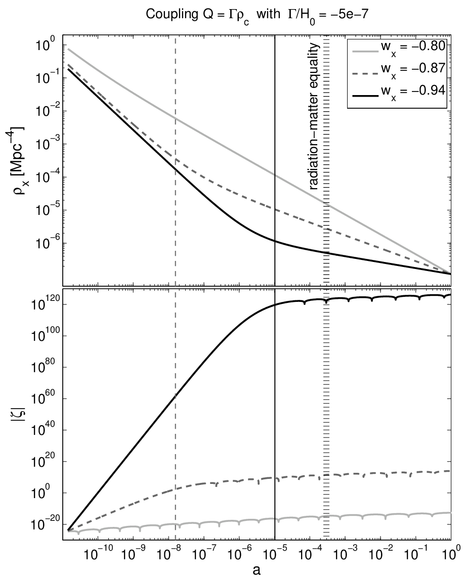
The analytical demonstration of the large-scale instability at early times is confirmed by numerical solutions, using a modified version of CAMB. Examples are shown in Fig. 1. As long as the coupling modifies the background evolution, the curvature perturbation is extremely rapidly growing: $\zeta\propto a^{n_{+}}$ where $n_{+}$ is given by Eq. (73) during radiation domination. When the background starts to behave as uncoupled, the blow-up of $\zeta$ ends and it begins to oscillate about zero with large (and mildly) increasing amplitude.

Equation (73) shows that for large enough $w_{x}$, there are oscillations super-imposed on the super-Hubble blow-up mode: $-\sqrt{2/3}<w_{x}\leq-{4/5}$, where the upper limit comes from Eq. (74). See Fig. 1 for an example (left panel, with $w_{x}=-0.8$).

Figure 1 also shows that if $|\Gamma|$ is large enough to modify the background after radiation-matter equality, then $|\zeta|$ follows a matter-dominated attractor solution:

The background solution in the matter era that corresponds to Eq. (43) is