Dipolar spinor Bose-Einstein condensates
Abstract
Under many circumstances, the only important two-body interaction between atoms in ultracold dilute atomic vapors is the short-ranged isotropic -wave collision. Recent studies have shown, however, that situations may arise where the dipolar interaction between atomic magnetic or electric dipole moments can play a significant role. The long-range anisotropic nature of the dipolar interaction greatly enriches the static and dynamic properties of ultracold atoms. In the case of dipolar spinor condensates, the interplay between the dipolar interaction and the spin exchange interaction may lead to nontrivial spin textures. Here we pay particular attention to the spin vortex state that is analogous to the magnetic vortex found in thin magnetic films.
pacs
03.75.Lm, 05.30.Jp, 76.50.+gI Introduction
Experimental realization of dilute atomic Bose-Einstein condensates (BECs) has revolutionalized the field of ultracold atomic physics [1, 2, 3]. For the first time, we have a macroscopic quantum object that is amenable not only to exquisite experimental control, but also to detailed microscopic theoretical description. Early experiments on atomic BECs were all carried out in magnetic traps, where the atomic spin is polarized by external magnetic fields, and hence the atomic spin degrees of freedom is frozen (see, however, Refs. [4, 5]). The atoms, however, get their spin degrees of freedom back when they are trapped in off-resonant optical dipole traps [6], in which case all magnetic Zeeman sublevels of the ground state atom can be trapped. Such condensates are called spinor condensates. Collisions between atoms give rise to an effective spin exchange interaction [7, 8], which is analogous to the exchange term in the theory of magnetism. The spin exchange interaction leads to interesting coherent spin-mixing dynamics in spinor condensates, a phenomenon that has been both theoretical studied [9, 10, 11, 12] and experimentally observed [13, 14, 15, 16].
Experimentally, spinor BECs have been realized in 23Na and 87Rb. The ground state of both these atoms possesses a small magnetic dipole moment of , where is the Bohr magneton. For typical condensate density ( cm-3), this would yield a tiny magnetic dipolar interaction energy on the order of 0.1 nK per atom, which is a few orders of magnitude smaller than the total collisional interaction energy. Furthermore, it appears that the small dipolar strength would be completely overwhelmed by any finite temperature effect (typical temperatures in BEC experiments are nK). Consequently, it has long been thought that dipolar interactions in such systems can be safely ignored. Hence, experimental effort to achieve dipolar atomic condensate has been focused on other types of atoms, notably 52Cr [17, 18] which has a magnetic dipole moment of in its ground state.
Under a more careful inspection, however, the conclusion that dipolar interaction plays negligible role in alkali atoms becomes questionable. We realized a few years ago that dipolar interaction in spinor alkali condensates can play a more prominent role for the following reasons:
- 1.
Although the total collisional interaction strength is much larger than the dipolar interaction strength, the spin exchange interaction is not necessarily much stronger. Particularly, for hyperfine manifold of 87Rb, the dipolar energy can be as large as 10% of spin exchange energy, thus making a nontrivial contribution to the total spin-dependent energy.
- 2.
The spin-dependent interaction, although much weaker in magnitude than the spin-independent interaction, is a critical determinant of the magnetic properties of spinor condensates.
- 3.
The long-range and anisotropic nature of the dipolar interaction may further enhance its effects.
- 4.
A small finite temperature will not overwhelm the dipolar effects due to the fact that, in a condensate, the interaction effects enjoy a Bose-stimulation factor — the total number of condensed atoms. This same reasoning also explains the importance of the weak nuclear dipolar interaction in superfluid state of 3He [19].
This motivated us to carry out a detailed investigation of the dipolar effects in spinor condensates. Our studies have confirmed that rich physical phenomena can indeed be induced by the dipolar interaction.
In the following, we will first present the Hamiltonian that describes the system. We will then study the ground state properties. To this end, two approaches will be used. The first is the so-called single mode approximation — all spin components of the condensate are assumed to possess the same spatial wave function. Under this approximation, the Hamiltonian can be greatly simplified, which makes a full quantum mechanical study possible. The single mode approximation, however, assumes that the atomic spins are uniformly oriented in space. Its validity depends on the dipolar interaction strength, as well as other parameters such as the geometry of the trap potential. To go beyond the single mode approximation, we adopt a second approach — the mean-field calculation without any a priori assumption on the spatial wave functions. From this study we see that sufficiently large dipolar strength induces non-trivial spin textures in the ground state. The specific pattern of the spin texture is sensitive to the trap geometry. In particular, a pancaked-shaped trap favors the spin vortex state, analogous to the magnetic vortices found in magnetic thin films or disks.
II Hamiltonian of a dipolar spinor condensate
We consider condensed spin atoms trapped in an axially symmetric harmonic potential,
| (1) |
with being the trap aspect ratio, and the atomic mass. We have chosen the symmetry axis to be the quantization axis, . The atoms interact with each other via both short-range collisions and long-range magnetic dipolar interaction. Under a uniform magnetic field , the second quantized Hamiltonian of the system reads
where and represent the non-dipolar and dipolar part of the Hamiltonian, respectively, and are given by
| (2) | |||||
| (3) |
where is the spin angular momentum matrices, is a unit vector, and the field operator for spin component (or Zeeman sublevel) . The collisional interaction parameters are [7, 8]
where is the scattering length for two atoms in the channel with total spin angular momentum . Symmetrization of many-body bosonic wave function dictates that only the symmetric spin channels and 2 are involved. The dipolar interaction parameter is
with being the vacuum magnetic permeability, and the Landé g-factor. Finally, in Eqs. (2) and (3), and hereafter, it is assumed that the repeated indices are summed over.
The first line of Eq. (2) represents the single-particle part of the Hamiltonian, while the second line results from the two-body contact interaction. The term proportional to is symmetric in the spin indices and represents the spin-independent contact interaction. The term proportional to , on the other hand, is spin-dependent and represents the short-range spin-exchange interaction. The sign of determines the nature of the spin-exchange coupling: negative represents ferromagnetic coupling, while positive represents antiferromagnetic coupling. The expression of in Eq. (3) follows from the dipolar interaction potential between two magnetic dipole moments () located at spatial points and , respectively,
| (4) |
The spin-exchange term and the dipolar term describe two types of spin-dependent interactions. It is the interplay and competition between these two terms that give rise to a rich variety of spin textures.
III Ground state under single mode approximation: single-domain state
III.1 Hamiltonian under single mode approximation
The total Hamiltonian of the system as represented by Eqs. (2) and (3) is quite complicated. There exists, however, a powerful method that can greatly simplify the problem. This is the so-called single mode approximation (SMA). More specifically, we assume that the field operators can be decomposed as
| (5) |
where is a unit normalized spin-independent spatial wave function. Here we shall not worry about the specific expression of , which should be properly chosen to minimize the total energy.
Inserting Eq. (5) into Eq. (2), we have
| (6) |
where is the total particle number operator and is the total spin angular momentum operator. Following a similar procedure, we may obtain under the SMA:
| (7) | |||||
where , and are the polar and azimuthal angles of , respectively. Obviously, this form of is still quite complicated. However, here we can take advantage of the spatial symmetry of the system to further simplify the dipolar part. As we have adopted an axially symmetric trapping potential, which is indeed the case in most experiments, it is natural to assume that the spatial wave function possesses the same axial symmetry. Under this condition, it is not difficult to see that if we carry out the integral in polar coordinates, terms proportional to in Eq. (7) will not survive after integrating over the azimuthal angle . We therefore have
| (8) |
where is the number operator for spin-0 component.
The total Hamiltonian under the SMA is obtained by combining Eqs. (6) and (8). Since we are dealing with an isolated system, the total number of atoms is a constant. Therefore, we may neglect terms that only dependent on . Finally, we have [20, 21]
| (9) |
where the two coefficients are defined as
| (10) |

It is worth pointing out the trap geometry-dependence of the effective dipolar coefficient . If we choose to be the single-particle ground state of the harmonic potential , i.e.,
where we have used the harmonic oscillator length to be the units for length, the integral in can be carried out exactly:
In Fig. 1, we plot as a function of trap aspect ratio . One can see that the sign of depends on the trap geometry:
This provides a convenient control knob one can use to change the properties of or even induce phase transition in the system.
III.2 Ground state structure under the single mode approximation

Hamiltonian (9) is reminiscent of the Hamiltonian that describes a quantum magnet. The ground state can be obtained by diagonalizing (9). In the absence of the external magnetic field, i.e., , the phase diagram can be plotted in the parameter space as shown in Fig. 2(a). According to the nature of the ground state, we can divide the parameter space into three regions labelled as I, II and III. Region I represents a ferromagnetic phase with easy-plane anisotropy. The ground state wave function in this region can be written as , where we have used the standard angular momentum basis state such that
Region II represents a ferromagnetic phase with easy-axis anisotropy. The ground state wave function in this region can be written as with a two-fold degeneracy. In both Regions I and II, the atomic spins are aligned along the same direction, either in the transverse plane (Region I) or along the -axis (Region II). Region III, on the other hand, represents roughly an anti-ferromagnetic phase where atomic spins are entangled to form spin singlets. Here the ground state wave function has a slightly more complicated form: where the coefficients has in general to be calculated numerically. Several examples are given in Fig. 3. The mixing of different states is due to the term in the Hamiltonian. In principle, the term will have a similar effect in the other two regions I and II. However, its effect there is negligible for large particle numbers .

For comparison, we also present the corresponding phase diagram for the non-dipolar case () [9] in Fig. 2(b). Under this situation, the Hamiltonian is simply which possesses a full rotational symmetry in spin space. The ground state is determined by the sign of . It is an isotropic Heisenberg (anti-)ferromagnet if (). The effect of the dipolar interaction is therefore quite transparent: It breaks the rotation symmetry of the non-dipolar system and introduces magnetic anisotropy.
Next we investigate the effect of a uniform external field. In particular, we are interested in the critical field strength at which the system is fully polarized by the external field.
Longitudinal field — First consider a longitudinal field along the -axis. It is easy to see that under this condition, is still a constant of motion since it commutes with the Hamiltonian (9). Its effect in Region II is quite obvious: Any longitudinal field will break the degeneracy of the ground state in the absence of the external field and polarize the spins along the field. Therefore the critical field strength here is infinitesimally small. For Region I, the new ground state should have the form where the value of may be obtained by minimizing the energy
which yields
where denotes the largest integer no larger than . Critical field strength is reached when or
For Rb condensate, this would correspond to a field strength on the order of 0.1 mG. The critical field strength for Region III can be obtain in a similar manner. Here the ground state has the form . The critical field is given by

Transverse field — Next we consider a transverse field along, e.g., the -axis. Its effect in Region I is similar to that of a longitudinal field in Region II: any transverse field would fully polarize the system in Region I. For Region II, we can take a classical approach since here the total spin is macroscopically large (). Treat the spin as a classical magnetization vector with length and polar angle , we can write down the energy of the system as (neglecting the unimportant -term)
Minimizing the energy with respect to yields the optimal value for as
Hence the critical field strength is
For , the ground state is doubly degenerate as schematically shown in Fig. 4. When , the two degenerate states collapse into one and the system is fully polarized by the transverse field. We want to point out that, in a quantum mechanical treatment, the double degeneracy at will be lifted by quantum fluctuations, resulting in quantum spin tunnelling [22]. Such quantum effects will be important when is small.
Finally, for Region III, the ground state can again only be obtained numerically as a superposition of different angular momentum states. The critical field can be shown to be
III.3 Validity of single mode approximation
Our discussion so far is constrained within the SMA. As can be seen, the SMA is a powerful approximation from which rich physics can be derived. Now we want to address the important question of the validity of this approximation.
First we notice that the SMA implies that the spin orientation is position independent. To show this, we define the normalized spin vector as
where is the number density, and is the total spin density. Under the SMA, we have , and . Therefore, we have which is spatially invariant. This situation would correspond to the so-called single-domain state of a nanomagnetic material [23]. The spatially uniform spin orientation minimizes the short-range spin-exchange interaction, but does not in general minimize the dipolar energy which is most effectively reduced for closure domain structures. Obviously the single-domain state is thus stable when the exchange interaction dominates. When this is not the case, the exchange interaction will be frustrated by the dipolar interaction, rendering the single-domain state intrinsically unstable to various other magnetically ordered states. Armed with this insight, we conclude that the SMA is valid only when the dipolar strength is sufficiently small and hence cannot cover the whole spectrum of interesting quantum spin phenomena.
Our study confirms this conclusion. For large dipolar strength, the SMA is no longer valid and nontrivial spatial spin textures develop in the system. We shall now turn to this situation that goes beyond the SMA.
IV Beyond Single Mode Approximation: Spin Textures
IV.1 Mean-Field Equations
To go beyond the SMA, we need to calculate the wave functions for each spin component explicitly. To this end, we adopt the standard mean-field approach. Specifically, the field operators in (2) and (3) are replaced by their corresponding expectation values . The Hamiltonian thus becomes the energy functional:
| (11) | |||||
where and are the total number density and spin density, respectively. Minimization of the energy functional requires , which yields a set of nonlinear coupled partial differential equations for the condensate wave function :
| (12) | |||||
| (13) | |||||
| (14) |
where and the integral operator is given by
The ground wave functions are obtained by solving these equations using the imaginary-time evolution method, where the term involving the integral operator are dealt with using convolution theorem and fast Fourier transform.
IV.2 Phase Diagram

From this calculation, the validity of the SMA can be directly checked by comparing the wave functions . Phase diagrams such as shown in Fig. 5 can be obtained [24, 25]. Fig. 5(a) is the phase diagram for a ferromagnetic exchange coupling with in the absence of external magnetic field. Here we fix the ratio to be corresponding to the values of 87Rb. The phase diagram is plotted in the parameter space spanned by the trap aspect ratio and the ratio between the dipolar and the exchange interaction strength . A similar phase diagram for an anti-ferromagnetic exchange coupling () is plotted in Fig. 5(b). Here we use as in the case of 23Na.
From Fig. 5, we can make the following observation:
- 1.
For any given trap geometry, the SMA is only valid for sufficiently small dipolar strength, in full agreement with the qualitative argument we made in Sec. III.3.
- 2.
In the region where the SMA is valid, according to the nature of the wave function which determines the local spin vector , we can further divide the region into three subregions labelled as SMA-I, II and III. They correspond to Regions I, II and III shown in Fig. 2.
- 3.
The critical value of where the SMA becomes invalid is sensitive to the trap aspect ratio: it decreases as increases, i.e., when the trap becomes more and more pancake-shaped. This shows that the dipolar interaction plays a more prominent role in a pancake geometry, which is consistent with the observation in the study of magnetic materials — The dipolar interaction, normally weak enough to be ignored in bulk materials, plays an essential role in stabilizing long-range magnetic order in two-dimensional systems such as magnetic thin film [26].
- 4.
In the region where the SMA is invalid, we can also divide the region into three subregions labelled C, S and P. We will discuss each of these regions in more detail below.
IV.3 Ground State Beyond Single Mode Approximation

Now let us discuss in more detail the ground state structure of the spinor condensate in the region where the SMA becomes invalid. The phase diagram plotted in Fig. 5 shows that there are three regions labelled as C, S and P, which stands for cigar, spherical and pancake, indicating the geometry of the trap in which a particular type of spin texture is favored.
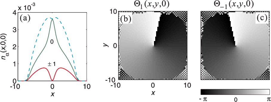
Figure 6 illustrates the ground state spin structure in these three regions. In a pancake-shaped trap (Region P of Fig. 5), spins are planar, i.e., lying in the transverse plane. Dipolar interaction forces the atomic spin to form a vortex pattern. We can write the wave function as . Our calculations show that in this region, the wave function contains a nontrivial phase:
| (15) |
where is a constant phase shift whose absolute value is not important but satisfies , is the azimuthal angle, and is then the “winding number” — circling once around the -axis, the phase of the wave function changes by . The specific values for the winding numbers are
Furthermore, we also have . Therefore, we can see that the spin component 1 and share the same density, but opposite winding number as illustrated in Fig. 7. The spin vortex state is obviously analogous to the magnetic vortex state found in magnetic thin films [23, 26]. However, there are important differences. In the central core region of a magnetic vortex, due to local magnetization conservation, the magnetic moment has to align perpendicular to the plane of the film in order to decrease the exchange energy at the center of the vortex. In a spinor condensate, however, there is no such constraint on local spin moments. Therefore local spin can simply vanish in the vortex core. Indeed, the core region is occupied by the spin-0 component while the other two spin components vanish. The spin vector can be expressed as
Such a spin texture is also referred to as a coreless skyrmion. Further, the spinor condensate is really a novel superfluid described by macroscopic wave functions which contain both amplitude and phase. In quantum mechanics, the spatial non-uniformity of the phase of a single-particle wave function is directly related to the velocity of the particle as
We therefore conclude that, in the spin vortex state, spin components 1 and circle around the -axis in opposite directions, while the spin-0 component is stationary as . This results in a situation with a net spin current but without a mass current.
In a cigar-shaped trap (Region C of Fig. 5), local atomic spins are predominantly aligned along the -axis. In that way, most of the spins are aligned in a head-to-tail configuration which minimizes the dipolar energy. Here the phase of the wave functions can still be expressed as in Eq. (15) but with a different set of winding numbers
Further the phase shift are no longer constants but functions of . The spin vector in the C phase takes the form
where , and is the spin twisting angle which is a monotonically increasing function of with .
In between the P and C phases, is the S phase which occurs when the trapping potential is close to spherical (). A distinct feature of the S phase is that becomes non-axisymmetric, signalling the breakdown of the cylindrical symmetry of the spatial wave functions. A typical spin configuration in S phase is displayed in the middle plot in Fig. 6. One can clearly see that the spin structure does not possess the cylindrical symmetry and there is a 180∘-domain wall separates two spatial regions of spin.
IV.4 Spin Vortex in External Magnetic Field
We have seen now that the dipolar interaction plays a more important role in pancake-shaped traps in which the ground state takes the form of a spin vortex. In this section we will focus on the spin vortex state and study how it responses to an external magnetic field.

Longitudinal field — First consider a uniform magnetic field along the -axis. Here we define the magnetization as
We plot in Fig. 8(a) the magnetization as a function of the field strength . As expected, the magnitude of is a monotonically increasing function of ( is negative here, because for the hyperfine level of alkali atoms, ). However, there exists a critical field strength at which suddenly jumps, signalling a first-order phase transition of the system. This critical field strength depends on the trap aspect ratio, the total number of atoms and the dipolar strength, as shown in Fig. 8(b).

To provide more insights into this phase transition, we study the wave functions . We find that the phases can still be written as in Eq. (15). The phase shifts always satisfy the condition . However, for , are constants; while for , become functions of as shown in Fig. 9. Furthermore, the winding numbers also change across the critical field and are given by
The local spin vector takes the form
with . For , we have ; while for , is a function of as shown in Fig. 9.
Transverse field — Now we consider the effect of a uniform transverse field along the -axis. As the field strength increases, similar to what happens in nanomagnets [27], the spin vortex starts to move away from the center and perpendicular to the applied field (along the -axis), and eventually moves out of the cloud. This is illustrated in Fig. 10.

V Conclusion
To conclude, we have shown that dipolar interaction plays a crucial role in spinor condensates. We have provided here a detailed study of the dipolar spin-1 condensate both within and beyond the single mode approximation. In the SMA regime, the system is analogous to the single-domain state of a magnetic material with the spins uniformly oriented. For sufficiently large dipolar interaction strength, the SMA becomes invalid, and spin textures develop as a result of the interplay between the exchange and the dipolar interaction. We have found that a pancake-shaped condensate is particularly sensitive to the dipolar interaction. In such systems, the spin texture takes the form of a spin vortex which is analogous to the magnetic vortex observed in thin magnetic films.
We have emphasized the connection between dipolar spinor condensates and ferromagnetic materials. We should also point out that there exist important differences between the two: While the latter represent a classically ordered system, the former are intrinsically quantum mechanical, as Bose condensates are macroscopic quantum objects described by quantum mechanical wavefunctions. Indeed we have seen that the spin vortex of a spinor condensate is intimately coupled with the topological charge of the condensate wavefunction: the spin components possess quantized vorticity or persistent currents. The fact that the spin textures and the motion of the atoms are intimately connected is a manifestation of an important property of the dipolar interaction, that is, the dipolar interaction provides a spin-orbit coupling. This can be more clearly seen if we notice that the dipole-dipole interaction potential (4) transforms as spherical tensors of rank 2 in both coordinate and spin space, and may be cast into the following form:
where is a spherical harmonic of rank 2 and its counterpart in spin space with components given by
The dipolar interaction is invariant under simultaneous rotations in coordinate and spin space and therefore conserves the total angular momentum (spin orbital). However, it does not conserve separately the spin and orbital angular momentum. The spin-orbit coupling induced by dipolar interaction also creates the opportunity for the transfer of angular momentum between the spin and the orbital degrees of freedom under the constraint of total angular momentum conservation. This could lead to the Einstein-de Haas effect in the dynamical evolution of a spinor condensates [28, 29]. Spin-orbit coupling effect has also been predicted in ferromagnetic nanostructures [30].
Finally, we want to mention that the Berkeley group led by Stamper-Kurn have developed a wonderful technique capable of non-destrctive in situ imaging of local spin textures in atomic condensates [31]. Using this technique, they have recently found tentative evidence of dipolar effects in spinor condensate of 87Rb [32]. To summarize, dipolar spinor condensates represent a novel class of anisotropic superfluid as well as a new kind of magnetic material, many of its rich properties are just starting to be explored.
Acknowledgements.
We acknowledge the financial support from US National Science Foundation under the Grant No. PHY-0603475 (HP), and from the National Science Foundation of China under Grant No. 10674141 and the “Bairen” program of CAS (SY).References
- [1] M. H. Anderson, J. R. Ensher, M. R. Matthews, C. E. Wieman and E. A. Cornell, Science 296, 198 (1995).
- [2] C. C. Bradley, C. A. Sackett, J. J. Tollett and R. G. Hulet, Phys. Rev. Lett. 75, 1687 (1995).
- [3] K. B. Davis, M. -O. Mewes, M. R. Andrews, N. J. van Druten, D. S. Durfee, D. M. Kurn and W. Ketterle, Phys. Rev. Lett. 75, 3969 (1995).
- [4] Tomoya Isoshima, Mikio Nakahara, Tetsuo Ohmi and Kazushige Machida, Phys. Rev. A 61, 063610 (2000).
- [5] P. Zhang, H. H. Jen, C. P. Sun, and L. You, Phys. Rev. Lett. 98, 030403 (2007).
- [6] D. M. Stamper-Kurn, M. R. Andrews, A. P. Chikkatur, S. Inouye, H.-J. Miesner, J. Stenger and W. Ketterle, Phys. Rev. Lett. 80, 2027 (1998).
- [7] T.-L. Ho, Phys. Rev. Lett. 81, 742 (1998).
- [8] T. Ohmi and K. Machida, J. Phys. Soc. Jap. 67, 1822 (1998).
- [9] C. K. Law, H. Pu and N. P. Bigelow, Phys. Rev. Lett. 81, 5257 (1998).
- [10] H. Pu, C. K. Law, S. Raghavan, J. H. Eberly and N. P. Bigelow, Phys. Rev. A 60, 1463 (1999).
- [11] H. Pu, S. Raghavan and N. P. Bigelow, Phys. Rev. A 61, 023602 (2000).
- [12] Wenxian Zhang, D. L. Zhou, M.-S. Chang, M. S. Chapman and L. You, Phys. Rev. A 72, 013602 (2005).
- [13] J. Stenger, S. Inouye, D. M. Stamper-Kurn, H.-J. Miesner, A. P. Chikkatur and W. Ketterle, Nature (London) 396, 345 (1998).
- [14] T. Kuwamoto, K. Araki, T. Eno and T. Hirano, Phys. Rev. A 69, 063604 (2004).
- [15] H. Schmaljohann, M. Erhard, J. Kronjäger, M. Kottke, S. van Staa1, L. Cacciapuoti, J. J. Arlt, K. Bongs and K. Sengstock, Phys. Rev. Lett. 92, 040402 (2004).
- [16] M. Chang, Q. Qin, W. Zhang, L. You and M. S. Chapman, Nature Phys. 1, 111 (2005).
- [17] A. Griesmaier, J. Werner, S. Hensler, J. Stuhler and T. Pfau, Phys. Rev. Lett. 94, 160401 (2005).
- [18] T. Lahaye, T. Koch, B. Fröhlich, M. Fattori, J. Metz, A. Griesmaier, S. Giovanazzi and T. Pfau, Nature (London) 448, 672 (2007).
- [19] D. Vollhardt and P. Wölfle, The Superfluid Phases of Helium 3 (Taylor & Francis, London, 1990).
- [20] S. Yi, L. You and H. Pu, Phys. Rev. Lett. 93, 040403 (2004).
- [21] S. Yi and H. Pu, Phys. Rev. A 73, 023602 (2006).
- [22] H. Pu, W. Zhang and P. Meystre, Phys. Rev. Lett. 89, 090401 (2002).
- [23] A. Hubert and R. Schäfer, Magnetic Domains (Springer, Berlin, 1998).
- [24] S. Yi and H. Pu, Phys. Rev. Lett. 97, 020401 (2006).
- [25] Y. Kawaguchi, H. Saito and M. Ueda, Phys. Rev. Lett. 97, 130404 (2006).
- [26] K. De’Bell, A. B. Maclsaac and J. P. Whitehead, Rev. Mod. Phys. 72, 225 (2000).
- [27] C. L. Chien, F. Q. Zhu and J.-G. Zhu, Phys. Today, June 2007, Page 40.
- [28] Y. Kawaguchi, H. Saito and M. Ueda, Phys. Rev. Lett. 96, 080405 (2006).
- [29] L. Santos and T. Pfau, 96, 190404 (2006).
- [30] K. Nakamura, T. Ito and A. J. Freeman, Phys. Rev. B 68, 180404(R) (2003).
- [31] J. M. Higbie, L. E. Sadler, S. Inouye, A. P. Chikkatur, S. R. Leslie, K. L. Moore, V. Savalli and D. M. Stamper-Kurn, Phys. Rev. Lett. 95, 050401 (2005).
- [32] M. Vengalattore, S. R. Leslie, J. Guzman and D. M. Stamper-Kurn, pre-print, arXiv:0712.4182 (2007).