Rise of the centrist: from binary to continuous opinion dynamics
Abstract
We propose a model that extends the binary “united we stand, divided we fall” opinion dynamics of Sznajd-Weron to handle continuous and multi-state discrete opinions. Disagreement dynamics are often ignored in continuous extensions of the binary rules, so we make the most symmetric continuum extension of the binary model that can treat the consequences of agreement (debate) and disagreement (confrontation) within a population of agents. We use the continuum extension as an opportunity to develop rules for persistence of opinion (memory). Rules governing the propagation of centrist views are also examined. Monte Carlo simulations are carried out. We find that both memory effects and the type of centrist significantly modify the variance of average opinions in the large timescale limits of the models. Finally, we describe the limit of applicability for Sznajd-Weron’s model of binary opinions as the continuum limit is approached. By comparing Monte Carlo results and long time-step limits, we find that the opinion dynamics of binary models are significantly different to those where agents are permitted more than 3 opinions.
keywords
Opinion dynamics, social and economic systems.PACS
PACS Nos.: 89.65.-s, 89.75.-k, 89.65.Ef1 Introduction
A recent revival of the study of social physics has been motivated by the hope that qualitative understanding of the mechanisms of human activity can be gained by constructing minimal models of interpersonal interaction [1, 2]. A number of ‘standard models’ have been introduced to describe diverse subjects such as opinion dynamics, traffic flow, financial transactions, structure of businesses, segregation and globalization. In this article we develop a continuum extension to a model of binary opinion evolution.
We begin this article with a brief overview of approaches that have been used to study opinion dynamics. Crucial to the current article, we start with the binary ‘United we Stand, Divided we Fall’ (USDF) model (sometimes known as the Sznajd model) which is a lattice based approach [3]. The binary USDF model originated as a modified Ising system, where up-spins map to opinion A and down-spins to opinion B. A simple rule set is used to modify the opinions of randomly selected pairs of agents on each time step. If a set of neighbors share the same opinion, then their neighbors are influenced and take on that opinion. If the neighbors have opposing opinions, then their neighbors also take on opposing opinions. The ‘community’ is closed, meaning that there are no external influences on the agents.
In the binary USDF model, relaxation times (time taken for average opinion to change from a majority of As to a majority Bs) were found to be in the region of 10000 time steps. It was observed that avalanches of opinion changes could follow from single opinion changes. There are three possible stable solutions at large timestep. Either the whole population of agents takes the opinion A, the entire population evolves to opinion B or an alternating opinion (solution with modulated opinion, ...ABAB...) is reached 11 1 In analogy to the ising model, some authors call this an antiferromagnetic solution. The relationship between the ratio of A and B opinions at the start of the simulation and the large timestep outcome was investigated, leading to the conclusion that an initial concentration of 70% A opinions is required to guarantee a final state of all A. To simulate the effects of influences beyond a closed community, ‘social noise’ was introduced, where opinions change at random with probability on each time step, leading to indefinite opinion fluctuations. Stauffer et al. extended Sznajd-Weron’s model to represent opinion dynamics on a square lattice [4].
Using the Sznajd model as a basis, Fortunato developed a continuum model [5]. Since the Sznajd model has only two opinions, it is of clear interest to develop a model with multiple opinions. Fortunato developed a model for a continuous set of opinions by using an agreement parameter to determine if agents interact [5]. Initially all agents are assigned random numbers representing opinions on a continuum between and . If two neighbors’ opinions agree to within this parameter then they are considered ‘compatible’ and a mean of their opinion is taken and mapped onto the surrounding neighbors. The update rule in Fortunato’s model is similar to that of Deffuant et al. if Deffuant’s convergence parameter is set to [6].
The justification for an agreement parameter is that people tend to form interest groups with others of similar viewpoint, and in that way are in a better position to propagate their view. In Fortunato’s model, only those who are willing to discuss their opinion (i.e. agents that have compatible opinions) are able to propagate their opinions. The results of Fortunato are interesting; however, in our opinion the model of Fortunato is not in the spirit of USDF models where agents of strongly differing opinion have a symmetric influence on the opinions of the population 22 2 In Fortunato’s article, there is a brief discussion of interactions between agents where opinions are outside the tolerance of the agreement factor. Thus, the polarizing effects of confrontation are not fully considered. We return to this point in section 2.2. We discuss the detailed rules of the binary USDF model and our extension to it in section 2.1. For completeness, we also mention that alternative binary and ternary models have been introduced by Galam [7] and Gekle et al. [8] respectively.
Network models of opinion dynamics have also been constructed. Effective descriptions of the social networks within populations have recently been developed [9]. Stauffer and Meyer-Ortmanns proposed a model of opinion dynamics which describes the interaction between agents on a scale-free network [10], drawing on an earlier model of Deffuant et al [6]. Update rules are similar to those used in Fortunato’s extension of Sznajd-Weron’s model [5].
This article is set out as follows. In section 2, we describe the detailed rules of the binary USDF model (section 2.1). Then in section 2.2, we discuss what we believe to be the most faithful continuum extension to Sznajd-Weron’s model, introducing a ruleset which leads to a true USDF model with persistence of opinion (memory) and that handles centrists in a consistent manner. We present results from Monte Carlo simulations of the continuum model in section 3.1 and simulate how the model evolves when the opinions of the agents are changed from binary through multi-state to continuum in section 3.2. Finally, we summarize our results and discuss possibilities for further extensions to the model in section 4.
2 Developing a continuum USDF model
2.1 The binary USDF model
The binary USDF Model [3] is a modified Ising model for simulating opinion dynamics where ‘spins’ represent opinions. The model community is set up as a set of agents , each of which have “opinions” chosen independently and at random from the discrete values . The agents exist on a chain with periodic boundary conditions. In the following, we use to represent binary opinions (the same notation as Sznajd-Weron). Continuous opinions are represented by . Once a population has been set up, pairs of neighboring sites at lattice points and are chosen at random on each timestep, , and the following rules are applied.
- Rule S1
-
Agreement: If a near-neighbor pair chosen at random has the same opinions then the next-nearest neighbors take on those opinions.
- Condition S1
-
If then apply Update S1.
- Update S1
-
and .
- Rule S2
-
Disagreement: If a pair chosen at random has opposite opinions then the surrounding neighbors take on opposing opinions.
- Condition S2
-
If then apply Update S2
- Update S2
-
,
The model can be written with a single rule which is applied on each timestep (, ), as was noted by Behera and Schweitzer [11]. This indicates that the model is trivial in the large timestep limit, since the lattice can be separated into two sublattices, with a ferromagnetic configuration always forming on a single sublattice. Therefore there are 3 outcomes: (a) Both sublattices have average opinion, (b) Sublattices have opposite average opinions - there are two configurations with this type of order, and thus (c) Both sublattices have . While Sznajd-Weron’s model may be trivial in the large timestep limit, we believe that the “united we stand, divided we fall” sentiment of the model is interesting, and have aimed to properly include the basic idea in a continuum extension.
2.2 Developing an extended model of continuous opinions
A key factor of the binary USDF model is that it is not only agents with similar opinions that interact and propagate their opinions; agents with diametrically opposed opinions may also interact. Our motivation is to develop a model with continuous opinions with the same core idea. We use the binary USDF consensus model [3] as a base from which to develop, and introduce a set of rules modified from those of a previous continuum extension developed by Fortunato, which only included propagation of similar opinions [5].
In the model of Fortunato [5], an agreement is defined if two opinions are within a set margin, i.e. . (In some regards, this is quite similar to Axelrod’s cultural propagation model [12]). We also want to include both the continuum nature of Fortunato’s model and an interaction between strongly conflicting agents similar to that in Sznajd-Weron’s USDF model. The most symmetric way of doing this is to define a disagreement if , where is a tolerance defining when opinions are of similar magnitude (we call the agreement parameter). It is easy to see that if neighboring opinions are nearly exactly opposite, this condition holds.
In Ref. [5], only agreement is treated in this way. There is a brief discussion of the disagreement required to provoke a “divided we fall” response in Ref. [5], but where that was implemented in Ref. [5]’s model it was assumed that any pairs of agents that do not agree, disagree, and the neighboring agents then take on the staggered alternating opinions of the pair of agents (this is equivalent to always making the map and without a test). We do not feel that this is in the spirit of the the binary USDF model, since there is not symmetry between strong disagreement and strong agreement. We introduce disagreement in the most symmetric extension to the agreement rule in Rule 2, which is one of the main differences between our model and Fortunato’s (there are also other differences as discussed in this section).
- Rule 1
-
(Agreement) If two agents have opinions that agree to within a certain margin, then they are said to agree. Then their average opinion propagates to neighboring sites.
- Condition 1
-
If then update opinions with update 1.
- Update 1
-
- Rule 2
-
(Disagreement) If two agents have opinions that are opposite to within a certain margin, then they are said to disagree. Then their difference in opinion propagates to neighboring sites.
- Condition 2
-
If then update opinions with update 2.
- Update 2
-
Therefore, there is a slight additional bias in the model towards the propagation of groups of agents with strongly opposed opinions. A motivation for this rule is that if there are strong disagreements between groups with diametrically opposed opinions, other agents are polarized into opposing viewpoints. There may be examples of such spreads (for instance in clashes between communists and fascists in inter-war Europe, or during conflicts between tribal groups where a positive feedback mechanism causes small frictions to turn into large disagreements) although we prefer to leave interpretation of the rule set to social scientists.
We note that the binary USDF model is not able to take into account the effects of intrinsic persistence of opinion (we call this memory)33 3 We note that the phrase ‘persistence of opinion’ is used to denote an extrinsic quantity relating to the length of time between opinion flips in some articles [13]. Using a continuum model is an excellent opportunity to include persistence effects. Memory is a strong characteristic of opinion dynamics and we believe that at least an investigation of its effects on the model is important. Using a memory factor means that the way an opinion is modified between timesteps is determined from both the initial opinion of the agent and updates 1 and 2 of the continuum USDF model. Therefore an agent’s opinion does not switch from one end of the opinion scale to the other instantly; rather the agent requires persuasion over a number of timesteps. The simplest way of implementing memory is to take a linear combination of the existing opinion and the opinion determined from updates 1 or 2. This can only be implemented in the continuous version of the USDF model, and not in the binary version (since the value of does not exist in the set of opinions used in the binary model), showing one of the advantages of our implementation.
To introduce a memory factor we make the following modification to updates 1 and 2,
- Rule M1
-
Agreement rule modified for persistence of opinion
- Update M1a
-
- Update M1b
-
- Rule M2
-
Disagreement rule modified for persistence of opinion
- Update M2a
-
- Update M2b
-
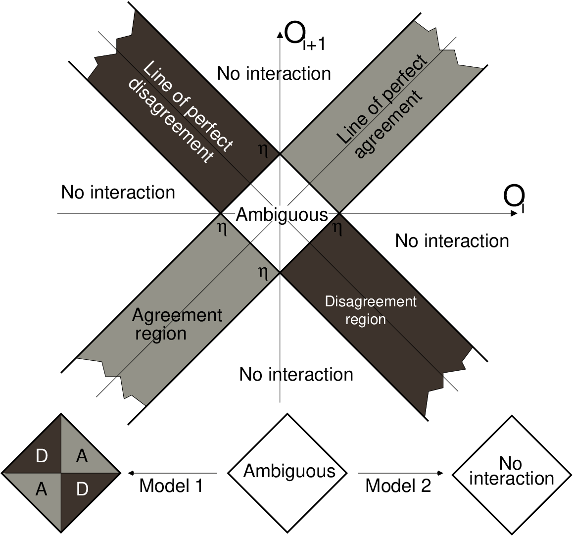
such that in a system where all agents have opinions with same magnitude, the total strength of opinion does not grow or shrink spontaneously. The index in the notation relates to the generation (time step) of opinions. denotes how much relative influence memory or interaction with neighboring agents has on the new generation of opinions. We summarize the pairwise interaction in figure 1.
2.3 An Ambiguous Region
The new rule set has an area of ambiguity for opinions of weak magnitude, since there is a small region of the interaction where both conditions 1 and 2 apply. The opinions that lie within this region are all smaller in magnitude than the agreement parameter and occur when . In this way, they can be thought of as representing centrist opinions. This can clearly be seen in figure 1; within the central region of the graph. We treat this region separately. There are two ways to deal with the low opinion region (a) interacting centrists (active centrist model) and non-interacting centrists (lazy centrist model).
2.3.1 Active centrist model (ACM)
A simple way to remove the ambiguity that arises for weak opinion is to treat separately the area where both conditions 1 and 2 are satisfied. Our first option for determining if agreement or disagreement rules should be applied is in keeping with the binary USDF Model [3]. We split the low opinion region into quadrants, so that the sign of the product of the opinions determines the type of update. A positive product is defined as agreement, and a negative product is defined as disagreement.
- Rule A
-
Additional rule for ambiguous region of ACM when .
- Condition A1:
-
There is agreement if so use update M1
- Condition A2:
-
There is disagreement if so use update M2
We call this set of rules the active centrist model (ACM). There is a direct mapping to the binary USDF Consensus Model when if we make the substitution .
2.3.2 Lazy centrist model (LCM)
An alternative way of treating weak opinions is to make no update if an opinion pair falls within the ambiguous region. We call this disambiguation the ‘lazy centrist model’ (LCM). The evolution of this model may be of interest to study disinterested voters. We note that both “active centrist” and “lazy centrist” variants are identical to the binary USDF model if the population of agents is initialized with only , and .
2.4 Algorithm and implementation
To simulate the model, we use a simple Monte Carlo algorithm to investigate how a population of opinions evolves over a period of time. The program was written in Mathworks MATLAB which offers a long period random number generator of the order , and a number of nice prepackaged routines for analyzing the resultant configurations of agents (e.g. convenient histogram routines).
Each run of the simulation is initialized on a 1D lattice, with each site allocated a random opinion from to . For the continuum model, opinions are allocated with a uniform random variate. For the discrete-opinion model, the opinions are initialized with
| (1) |
where is the total number of opinions, and is a uniform integer variate with levels (parameters of and ensure that only opinions of the same magnitude interact). There is a choice of boundary conditions. Our population of opinions exists on a ring (i.e. 1D chain with periodic boundary conditions). Considering that the model that we propose is highly simplified, the choice of boundary conditions is expected to be unimportant in comparison to other simplifications (e.g. lattice vs network).
After the initial setup of the population, we simulate using a Monte Carlo method. Our simulation uses sequential rather than concurrent updating, where a pair of the population is selected at random on each time step. The algorithm finishes when a certain preset number of time steps have been completed. When we calculate ensemble averages, typically we simulate 10000 ensembles each with a different random starting population.
The algorithm can be summarized as follows:
- 1.
Initialize the population with random opinions (spins), either with continuous or discrete opinions.
- 2.
Choose a pair of neighboring spins from the total population
- 3.
Determine the required update step:
- (a)
If the opinion pair is in the ambiguous region (condition A is satisfied), update next-neighbor opinions according to Rule A (ACM) or do nothing (LCM).
- (b)
Otherwise, update using rule 1 or rule 2.
- (a)
- 4.
- 5.
Restart at step 1 until the ensemble of runs is large enough for meaningful statistical averages.
3 Results and Discussion
3.1 Properties of the continuum model
3.1.1 Evolution of opinions
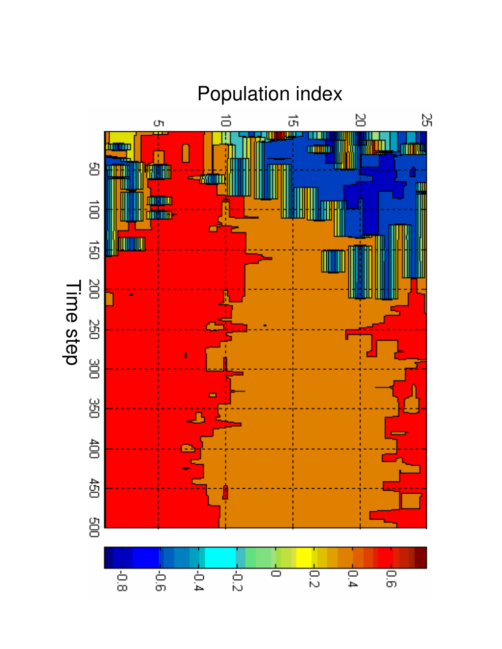
We demonstrate the inner workings of our “society” of agents by following the evolution of all the individual opinions in a single run, shown in figure 2 as a density plot of the opinion of each agent vs time step. A small population of agents is simulated, using the LCM ruleset with agreement parameter , no persistence of opinion () over a period of 500 timesteps. Each location on the -axis represents an individual agent and time progresses along the -axis. The -axis (color) represents opinion. As expected, opinions are diverse at the beginning of the simulation, since they have been initialized randomly. Over the course of the simulation, patches of monotonous opinions become dominant. Towards the end of the run shown in the figure, the opinions converge to two regions of similar positive opinion. Since the opinions are similar enough to continue interacting, it is expected that a single opinion will eventually emerge. We believe the origins of opinion domains to be similar to those in Axelrod’s model of cultural evolution [12]. The regions of modulated opinion that can be seen early in the simulation become extinct by just over 200 time steps. This coincides with a flip from negative to positive opinion values. Before timestep, , a greater proportion of society is at the ‘blue’ end of the opinion scale. Within a small number of time steps, the number of red opinions increases dramatically. By , the ‘blue’ opinions are almost eradicated. This characteristic behavior is also seen in the binary USDF model [3].
3.1.2 Average opinion

Figure 3 shows the evolution of the average opinion of a different population of agents during a single run over 10000 loops. The population size was agents with an agreement parameter of and no memory effects (). The ACM rule set was used. Only a very small change in the average opinion was seen, however it is interesting to note that there were several intersections with the -axis during the simulation. The swing from positive to negative opinion took place over about 4000 time steps. It is important to remember that results obtained from single runs are not predictive.
3.1.3 Distribution of average opinions
In this section, we analyze the distribution of average opinions. After a designated number of time steps, the average opinion of a single run is calculated. After 10000 ensemble runs, these averages are binned into a histogram. We use histograms to analyze the ensemble since it gives more information than the computation of a simple average or standard deviation. For instance, non-Gaussian distributions can be assessed. We show histograms computed for simulations with no memory factor () in figure 4. The effects of the memory factor on the distribution are shown in figure 5.


The results in figure 4 can be directly compared with the binary USDF model. The binary USDF model [3] has three long time steady states, so if the continuum extension to the model has no effect, we would expect the distribution of average opinions computed after a large number of time steps to be 3 peaked (we confirm this later in the article). Clearly, our model has quite a different distribution of opinions, with a broad single peaked structure. In the LCM, increase in broadens the distribution. In particular, panel (f) shows that the probability distribution may be spreading into 2 peaks. The spread in the distribution is expected in the LCM rules, since agents with may not propagate their opinion, and so become extinct in the large time step limit. In contrast, little change is seen in the ACM as is changed. The different behavior of our model could be a result of several factors. Either a steady state has not been reached, or the binary USDF Consensus Model breaks down as a set of continuous opinions are reached, with the absence of extreme opinion sets. We revisit this point later in the article.
Figure 5 shows the effect of memory. In both the LCM and ACM models when a memory factor of is used, the distribution of average opinions is halved. In the limiting case of , the distribution of opinions may not change. This indicates that one of the effects of memory is to increase the time scale in the model. A secondary effect of memory on the LCM is non-trivial. Consider a pair of agents that agree with positive opinion sitting next to an agent with . The effect of the influence of the first pair is to change the opinion of the agent to . Thus, persistence of opinion causes new opinions to be created, which can have value , so there is a constant flux between creation and extinction of centrist views in the LCM with persistence of opinion.
3.1.4 Variance of average opinions

In order to gain greater insight into the distribution of opinions, we study the time evolution of the variance. Figure 6 shows the evolution of the variance of average opinions for various agreement parameters, clarifying what is seen in figure 4. The average variance typically reaches a plateau within 10000 timesteps. The large timestep variances of opinions that the models with and reach are very similar. The variance drops dramatically above . In the simulation where , neighbors pairs can only convince their neighbors once they have a magnitude of opinion greater than . This explains the rapid initial increase in variance for large , which is the result of the extinction of agents with centrist views. For all interactions are via the ambiguous rules - thus no LCM updates are permitted, and the variance shows no change with time step.
3.2 Comparisons with the binary USDF Model
The results presented in the previous section have shown that it is necessary to make a further analysis of the absence of the 3 peak structure in the density of long time scale average opinions (since that is the structure in the binary model). To make this analysis, we adjust our simulation to have only discrete opinions following equation 1. The adjustments are minor. In the binary case, we simply initialize with and choose appropriate model parameters so that no intermediate sized opinions are created () where is the difference between closest opinion states. For the binary simulations, . We set , since any memory factor would generate non-binary opinions). We choose to simulate a set of agents with following the LCM rules (for the binary simulation with small , LCM and ACM are identical, since the ambiguous rules are never invoked). In order to investigate the long time step limit, we analyze a population of agents with time steps. Those parameters were determined empirically to represent a stable density of average opinions. We also have the opportunity to examine systems with other numbers of opinions. A ternary model can be formed by initializing (or yes, no, unsure set) where , but otherwise using the same parameters. Since we use the LCM rules, agents that are ‘unsure’ may not propagate their opinions. We also simulate a 5 state model where (strongly agree, agree, unsure, disagree, strongly disagree set). Again, since the LCM rules are used, the ‘unsure’ agents do not propagate their opinions.


Figure 7 was produced by binning the average opinion on the final time step of each run in the ensemble. It shows the evolution of the binary USDF model via 3 and 5 state models into a continuous model. Top left, 2 opinion, (Sznajd or binary USDF model), top right , bottom left and bottom right continuous opinions. Each simulation was carried out with a population of , loops over ensembles using the LCM rules with and .
There are significant differences in the density of average opinions formed in the different discrete models, as seen in figure 7. The binary USDF (Sznajd model) results (top left) show that a three peaked system emerges in the long time limit. This is expected as there are 3 possible stable outcomes to a binary system in the long timescale limit, either all the agents take opinion A, all the agents have opinion B or there is a perfect split, 50% of the agents taking each view on neighboring sublattices. This is a direct consequence of the disagreement rule, which allows the space modulated state with to form.
The same logic allows us to determine the steady states of a three-opinion population of agents. It is useful to understand which steady states we expect in the long time scale limit. The stable states of a three opinion model can be easily determined and are shown in the table (table 1). These are the states in which application of any of the update rules to any pair in the population leads to exactly the same configuration. Clearly the most obvious steady states are where all the members of the population have the same opinion. There are 3 of these in the ACM (all A, all B and all C), and 2 in the LCM (all A and all C, since in the LCM the B state becomes extinct as it is not able to propagate). In addition to these states, states with modulated opinion are stable, with two types of alternating A and C states (AC and CA). This distribution of average opinions matches the results from simulations of the 3 opinion model which we show in Fig. 7 (top right).
| \topruleModel and states | Steady state | Deg. |
| \colruleBinary, | all A (), all B () | 1 |
| A (=yes), B (=no) | alternating AB () | 2 |
| \colruleTernary, | all A (), all C () | |
| A (=yes), B (=unsure), C (=no) | or all B (ACM only ) | 1 |
| alternating AC () | 2 | |
| \colruleFive state, A (=strong agreement), | all A (), all B (), | |
| B (=agreement), C (=unsure), | all C (ACM only, ) | |
| D (=disagree), | all D () or all E () | 1 |
| E (=strong disagreement) | alternating AE () or BD () | 2 |
| \botrule |
We repeat the calculations for models with more opinion states. As can be seen in Fig. 7 (bottom left and right) for 5 or more opinion levels, little difference is found between discrete and continuous opinions. With a 5 state opinion base there is already a very high probability of producing a central average opinion. Here, we kept constant. However, if the limit was taken keeping , the result would be a flat continuous distribution with constant density (since half the end states have all agents exhibiting the same opinion, with weight ) and a -function spike at represents end states with modulated opinion, i.e. .
4 Concluding remarks
We have proposed an extension to the binary “United we stand, divided we fall” opinion dynamics of Sznajd-Weron, which can handle continuous opinion distributions. We used the most symmetric extension of the binary model in order to take account of the consequences of disagreement (confrontation) within a population of agents in conjunction with agreement (debate). We have also developed rules for persistence of opinion (memory) and for the propagation of centrist views. We carried out Monte Carlo simulations. Memory effects were found to significantly modify the variance of average opinions in the large timescale limits of the models. We described the breakdown of binary opinion dynamics on approaching the continuum limit. We compared Monte Carlo results with a consideration of long time-step steady states. Our main conclusion is that the outcomes of USDF models are strongly modified when agents are permitted more than 3 opinions.
Geographically the lattice approach is incomplete as influences of opinion are likely to form a complex network, combined with a local lattice and also global influences (e.g. the media). There are a number of possible directions for further studies. For example it might be interesting to extend the model to exist on the scale-free networks of Barbarási [9]. It is estimated that there is a high degree of connectivity in real-world networks, much greater than in the simple lattice where and the inter-agent distance is simply [9]. Choosing to place agents in networks rather than on lattices may lead to a more detailed description of opinion dynamics, although understanding long time scale behavior would be more difficult. Including external influences, non-conformists and global effects are all likely to improve insight. To finish, we would also like to point out that a simple propagation of average views of agents with similar magnitude opinions may not be sufficient. Sometimes the opinions of others are so extreme that they can polarize even centrists away from their views.
Acknowledgments
JPH would like to acknowledge support from EPSRC grant no. EP/C518365/1.
References
- [1] T. C. Schelling. Micro motives and Macro behaviour. W. W. Norton, New York, 1978.
- [2] P. Ball. Critical mass: How one thing leads to another. Farrar Straus Giroux, New York, 2004.
- [3] K. Sznajd-Weron and J. Sznajd. Opinion evolution in a closed community. Int. J. Mod. Phys. C, 11:1157, 2000.
- [4] D. Stauffer, A. O. Sousa, and S. Moss de Oliveira. Generalization to square lattice of sznajd sociophysics model. Int. J. Mod. Phys. C, 11:1239, 2000.
- [5] S. Fortunato. The sznajd consensus model with continuous opinions. Int. J. Mod. Phys. C, 16:17–24, 2005.
- [6] G. Deffuant, F. Amblard, G. Weisbuch, and T. Faure. How can extremism prevail? a study based on the relative agreement interaction model. Journal of Artificial Societies and Social Simulation, 5(4):1, 2002.
- [7] S. Galam. J. Stat. Phys., 61:943, 1990.
- [8] S. Gekle, L. Peliti, and S. Galam. Opinion dynamics in a three-choice system. Eur. Phys. J. B, 45:569, 2005.
- [9] A. L. Barbarási and R. Albert. Emergence of scaling in random networks. Science, 286:509–512, 1999.
- [10] D. Stauffer and H. Meyer-Ortmanns. Simulation of consensus model of deffuant et al. on a barbasi-albert network. Int. J. Mod. Phys. C, 15:241, 2004.
- [11] L. Behera and F. Schweitzer. On spatial consensus formation: Is the sznajd model different from a voter model. Int. J. Mod. Phys. C, 14:1331, 2003.
- [12] R. Axelrod. The dissemination of culture. Journal of Conflict Resolution, 41:203, 1997.
- [13] D. Stauffer and P. M. C. de Oliveira. Persistence of opinion in the sznajd consensus model: computer simulation. Eur. Phys. J. B, 30:587, 2002.