From the conserved Kuramoto-Sivashinsky equation to a coalescing particles model
Abstract
The conserved Kuramoto-Sivashinsky (CKS) equation, , has recently been derived in the context of crystal growth, and it is also strictly related to a similar equation appearing, e.g., in sand-ripple dynamics. We show that this equation can be mapped into the motion of a system of particles with attractive interactions, decaying as the inverse of their distance. Particles represent vanishing regions of diverging curvature, joined by arcs of a single parabola, and coalesce upon encounter. The coalescing particles model is easier to simulate than the original CKS equation. The growing interparticle distance represents coarsening of the system, and we are able to establish firmly the scaling . We obtain its probability distribution function, , numerically, and study it analytically within the hypothesis of uncorrelated intervals, finding an overestimate at large distances. Finally, we introduce a method based on coalescence waves which might be useful to gain better analytical insights into the model.
Keywords:
Nonlinear dynamics , Coarsening , InstabilitiesPACS
02.50.Ey , 05.45.-a , 05.70.Ln , 81.10.Aj1 Introduction
The study of growth processes of crystal surfaces [1, 2, 3] has turned out to be a source of a variety of nonlinear dynamics. A first, general distinction should be made between a crystal growing along a high symmetry orientation (e.g., the face (100) of iron) and one growing along a vicinal orientation (e.g., the face (119) of copper). In the former case, growth proceeds [4, 5] layer-by-layer via nucleation, aggregation of diffusing adatoms and coalescence of islands; in the latter, the surface is made up of a train of steps [6] which advance through the capture of diffusing adatoms (step-flow growth).
The interest in the nonlinear dynamics of a crystal surface mainly comes from the observation that growth is often unstable [7]. Step-flow growth plays a special role because it allows for rigorous treatments and the original two-dimensional character of the growth may reduce to effective one-dimensional equations: an equation for the density of steps when steps keep straight and an equation for the step profile, when steps move in phase. The two cases occur during step bunching [7] and step meandering [8, 9], respectively.
As for the nonlinear dynamics resulting from the instabilities, they may vary from spatio-temporal chaos [10] to the formation of stable structures [11], from coarsening processes [12] due to phase instabilities [13] to diverging amplitude structures [14]. Recently, T. Frisch and A. Verga have found [15, 16] that in special limits11 1 In the case of vanishing desorption and weak asymmetry in the attachment kinetics to the steps. the profile of the wandering steps satisfies the equation
| (1) |
now known as the conserved Kuramoto-Sivashinsky (CKS) equation. The “conserved” label becomes clear upon comparison with the standard Kuramoto-Sivashinsky eq., .
An equation similar to (1), with an extra propagative term , arises in step bunching dynamics with vanishing desorption [17] and in the completely different domain of sand-ripple dynamics [18]. The propagative term can be removed using the transformation , which, however, introduces dependent boundary conditions [17]. Numerics and heuristic/similarity arguments give a coarsening pattern whose typical length scale grows as , with a coarsening exponent , both in the presence [17, 18] and in the absence [15] of the propagative term.
The linear stability spectrum of the CKS eq. has the form . In many equations having the same , coarsening occurs because the branch of steady states has a wavelength which is an increasing function of the amplitude. These steady states are unstable with respect to phase fluctuations and the profile evolves in time, keeping close to the stationary branch [19].
For the above reason, our first step will be to discuss the periodic stationary states of the CKS eq. (Section 2), showing they look like sequences of arcs of a universal parabola, connected by regions of diverging curvature (asymptotically, angular points). Direct simulations of the CKS eq. [15] show that: (a) during the dynamical evolution, the interface profile can be thought of as a superposition of parabolas, and (b) the typical size of parabolas (in the direction) grows with time as .
In order to understand better the dynamics, we have simplified the problem, starting from the observation that angular points can be seen as effective particles interacting through the connecting arcs of the parabolas. The correspondence of a Partial Differential Equation (PDE) with a system of particles is known for the deterministic Kardar-Parisi-Zhang equation [20], where arcs of parabolas are separated by cusps. In that case, the PDE is linearly stable, which translates to parabolas of decreasing curvature. For the Burgers equation [21], cusps are replaced by shock waves and arcs of parabolas by linear pieces of decreasing slope.
In principle, the particles move in two dimensions (the plane) and each particle interacts with all other particles. This full description, if possible, would be exact. However, we keep things simpler by limiting to the horizontal motion and to nearest neighbour interactions. Therefore, in Section 3 we show that the dynamics of particles is described by the equations , where is the coordinate of the th particle and . When two particles collide (), they coalesce and the total number of particles decreases by one, thus leading to a coarsening process.
Subsequently, we simulate the particle model (Section 3.1) finding the coarsening law and the size distribution of interparticle distances, . A very crude approximation of the Fokker-Planck equation for the particle system (Section 3.2) gives the correct expression for , but overestimates at large . Finally, we introduce the method of coalescence waves (Section 3.3), finding some preliminary numerical results, which might guide a future, more rigorous analytical study.
2 Steady states
The steady states of the CKS equation (1) satisfy the second-order nonlinear differential equation Since the constant must vanish in order to get bounded solutions, while the constant can be trivially absorbed into a uniform shift of and be set to zero, the problem reduces to solving the differential equation
| (2) |
This equation also gives the steady states of a different PDE, studied by Mikishev and Sivashinsky [22]. Therefore, we limit ourselves to just a few results that play a major role in what is to follow.
Interpreting in Eq. (2) as time, the equation corresponds to a harmonic oscillator subject to an external force proportional to the velocity squared. Deriving (2) with respect to and putting , one obtains
| (3) |
Assuming the initial conditions and , the solution is
| (4) |
We then have the trajectories in the -phase space:
| (5) |
If the force is strictly negative and the trajectory is not limited. On the other hand, if , with , we get periodic, bounded trajectories, which oscillate between and . For , we obtain the separatrix , which corresponds to the parabolic trajectory . See Fig. 1 for more details.

It is useful to determine the amplitude in the negative direction, as a function of . For , it is easily found that , while in the important limit , diverges logarithmically according to , i.e.,
In proximity of , bounded trajectories have a minimum with a curvature that diverges as , as shown by the expansion in Eq. (5), which gives This approximation is shown as thin full lines in Fig. 1 (small upper inset). The quadratic and quartic terms are of the same order when , which sets the size of the high-curvature region. In fact, the slope joins the corresponding slope of the limiting parabola , when .
Finally, in the large lower inset of Fig. 1 we plot the wavelength of the steady states as a function of their amplitude . The full line, , gives the analytical approximation valid for large . It can be determined from the asymptotic parabola , imposing .
2.1 Steady states and dynamics
In the Introduction we have argued that steady states are important because dynamics proceeds by evolving along the family of steady states of increasing wavelength .22 2 This is both an observation (see the following discussion on Fig. 2) and a consequence of the stability of steady states with respect to amplitude fluctuations, see Ref. [19]. In the case of the CKS equation special attention should be paid to the constant and to the conserved character of Eq. (1). We now show how the conservation law fixes the value of , as a function of . We shall then argue that is the time-dependent vertical shifting of the surface profile.
On the one hand, the conserved dynamics requires that the spatial average is time independent; on the other hand, steady states found in the previous section have a non vanishing and -dependent average value. Therefore, the family of steady states which is relevant to the dynamics is where the constant satisfies the condition . For large , the average value of can be safely determined by approximating it with the arc of the (separatrix) parabola, so that
| (6) |
Therefore, for large we get .
3 The particles model
The following approach is founded on two observations, the first based on theory, the second on numerics: (i) When increasing the wavelength of steady states, tends to a sequence of arcs of the universal parabola , connected by regions of diverging positive curvature whose size is vanishing small. See Section 1 and Fig. 1. (ii) Dynamics deforms the above picture, but interface profiles can still be thought of as a sequence of points , with and the following properties: with increasing time, and between any pair of consecutive points can be approximated as an arc of the universal parabola, with and determined by the conditions and . See Fig. 3 of Ref. [15] and our Fig. 2.

Therefore points () (henceforth particles, full dots in Fig. 2) define unambigosuly the full interface profile and their dynamics should be derivable from the CKS eq. The coarsening process occurs because bigger parabolas eat neighboring smaller ones. When one parabola disappears, two particles merge into one: it is a coalescence process. Because of the conservation of the order parameter, , particles do not move independently and their effective interaction is expected to be fairly complicated and long-range.
Here we limit ourselves to a simple model where a single bigger parabola () eats a smaller one (), see Fig. 3 (full line). The full configuration is defined by the three parameters and , the point where the two parabolas meet. Two conditions must be fulfilled: continuity in implies and conservation implies . In this picture, the particle in has neighbouring particles at distances on the left and on the right.
The next step is to use the CKS eq. to evaluate : it is enough to multiply both sides of Eq. (1) by and to integrate. We get
| (7) |
where the last term on the right vanishes because of periodic boundary conditions. The average values and are evaluated using the two-arcs approximation depicted in Fig. 3 and are therefore functions of only. Once we replace by , we obtain a differential equation for the position of the particle,
| (8) |

The evaluation of and is straightforward, because the region of the angular point can be safely neglected:
| (9) | |||||
| (10) |
As for the average value , we may write where means the average on the angular point and is the abrupt change of slope occurring through the angular point, on a distance of order . Since , we get the term being negligible for large (which means large and small ).
For a periodic configuration of wavelength , we have . In the configuration of Fig. 3 we do not have a single , but the two quantities . If we assume , we get , with being determined by the condition that the right-hand-side of Eq. (7) vanishes for : in fact, the particle has zero speed in the symmetric configuration . So, we get It is worth stressing that a completely different assumption, , gives a result which is almost indistinguishable from this.
We now have to determine the derivative appearing at the denominator of Eq. (8): , so we finally get . Expressing in terms of the interparticle distances , we finally get , , and
| (11) |
This is one of the main results of the paper: it means that the conserved Kuramoto-Sivashinsky equation can be translated into the motion of a system of particles with attractive interactions, decaying as the inverse of their distance, and undergoing a coalescence process when they collide. If the coordinate of the th particle is , we can write
| (12) |
Alternatively, if is the distance between particles and , we get
| (13) |
Since interparticle force decays as the inverse of the distance, the coarsening law, i.e. the time dependence of the average distance between particles, , can be easily inferred from scaling considerations,
| (14) |
This result is in agreement with numerical simulations [15] of the CKS equation and with numerical results of the particle model, discussed in the following section. It will also be corroborated by the Fokker-Planck approach, Section 3.2. It is worth noting that the result is not related to diffusion since the particles motion is strictly deterministic; it arises from the decay of the interparticle force with distance .
3.1 Simulation of the particle model
Rather than solving Eqs. (12) for particle positions, we have solved Eqs. (13) for the distances. Fig. 4 shows that the expected law is satisfied for very different initial conditions: a random distribution (full diamonds) and a slightly perturbed uniform distribution (empty circles). The asymptotic value of is the same for the two distributions, showing that the prefactor in only depends on the initial density. The two sets (circles and diamonds) are distinct at small because the initial random distribution favours more coalescences at short times than the uniform one.
Fig. 5 shows the normalized distribution of interparticle distances as a function of . Again, widely different initial configurations produce the same asymptotic distribution (empty circles and diamonds). As for the limiting behaviors of , they are plotted in the upper inset for small and in the lower inset for large . At small we clearly have a power law distribution, , with exponent . At large , data seem to suggest a gaussian tail.
The qualitative features of the distribution can be understood by comparison with the one-species diffusion-limited coalescence process on the line [23]. In our case, particles separated by a smaller gap than average close the gap at increasingly larger speeds. As a result, the system evolves effectively as if nearest particle pairs react instantaneously, before the rest of the system evolves (numerical simulations do confirm this intuitive notion). In the diffusion-limited coalescence process, a quasi-static approximation shows that particle pairs react at a time proportional to the gap between them. Thus, both processes favor faster reactions between nearest particle pairs (in our case, more aggressively so). The distribution for diffusion-limited coalescence is known exactly, yielding for small , and a gaussian tail for large. It is not surprising that we find a similar . The faster-than-linear behavior, , in our case, is consistent with the faster reactions between nearest particle pairs, leading to a faster depletion of the probability distribution function near the origin.


3.2 The Fokker-Planck equation
In this Section we use the Fokker-Planck (FP) equation for the distances , under the approximation of uncorrelated intervals. The same approach has already been used for models of particles interacting with a force decaying exponentially, see Refs. [24, 25], and we refer the reader to those papers for more details.
If is the force between two particles at distance , Eq. (13) can be written as
| (15) |
and the FP equation for the probability to find a given distribution at time is
| (16) |
We are mainly interested in the time dependence of the average distance, , and in the probability distribution for the distances, , which is expected to have the asymptotic scaling form , with . In the approximation of uncorrelated intervals, we get the equation which does not include the coalescence process, because the form implies the conservation law . Details on how to include coalescence are very similar to published papers [24, 25] for different , so here we merely state the results:
| (17) | |||||
| (18) |
The expression for agrees with numerical results (Fig. 4) and with scaling considerations, Eq. (14). On the other hand, the results for do not match our numerical findings, discussed in Section 3.1, indicating the importance of correlations, neglected by this approach. The evolution equation (13) clearly shows that adjacent intervals are strongly anticorrelated, as gaps grow (or shrink) on expense of their surroundings; larger than typical intervals are surrounded by smaller than typical ones, and vice versa. Thus, larger than typical intervals grow far less than the independent interval approximation would allow, as the neighbors they engulf are typically smaller than average. In this way the approximation overestimates the frequency of long intervals (, instead of a gaussian tail). Similarly, being surrounded by large intervals, short intervals contract faster than if they were surrounded by typical intervals, explaining the overestimate of their frequency ( instead of ) by the approximation.
3.3 Coalescence waves
This final section is dedicated to preliminary results on the study of coalescence waves, which might be useful for a deeper understanding of numerical results for the particles model.
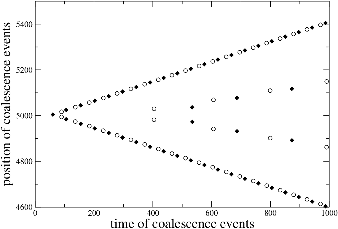

Consider a uniform distribution of particles, perturbed at a single point: for and . As the system evolves, according to Eq. (13), the perturbation propagates on both sides of its origin, leaving behind a trail of coalescence events. These coalescence events take place at roughly equally spaced locations and time intervals, defining an apparent “front”, see Fig. 6. The speed of the front (the slope of the straight line in the figure) is independent of the sign or magnitude of the perturbation, but seems to depend only on the density of background particles, , with . The frequency, or inverse time between two consecutive coalescence events is roughly , with . Therefore the coalescence front leaves a diluted system behind, with density , or about one half the original density. Following these events, a second front of coalescence events sweeps through, this time at roughly half the previous speed, due to the reduced density. This second front, clearly visible in Fig. 6, might be followed yet by others, but their quality deteriorates fast as the background of remaining particles distorts away from the original homogeneous spread.
Next, we ponder how two propagating fronts, originating from two distant perturbations, interact. In Fig. 7 we plot simulations results for this scenario. One can see that coalescence fronts propagating in opposite directions annihilate. We have confirmed that annihilation takes place even when the two perturbations are started at different times. The rules for front propagation and interaction seem very simple, and give us hope that they might prove useful in shedding light on the kinetics of initially disordered particle systems.
4 Summary
The initial motivation of our work was to study the so called Conserved Kuramoto-Sivashinsky equation, Eq. (1), whose stability linear spectrum is and whose numerical integration [15] gives a coarsening process with an exponent . The analysis of steady states (Sec. 2) tells us that stationary configurations have the form , where is a -periodic function satisfying the differential equation and is a constant fixed by the condition .
Numerics and theoretical background suggest that the function evolving according to the CKS eq. keeps close to steady states. More precisely (Fig. 2), appears to be similar to a continuous piecewise function, where each piece is a portion of the universal parabola . Actually, connecting points are vanishing regions of diverging positive curvature in the surface model. We have shown (Sec. 3) that these angular points can be thought of as effective particles and we derived the equations governing their dynamics, Eqs. (12,13).
Simulating the particles model is definitely easier than simulating the interface model and we have obtained (Sec. 3.1) the coarsening law and the distribution of interparticle distances. We also expect that future analytical treatment would sooner be addressed to the particles model and we suggest two main directions: first, using the Fokker-Plank equation beyond the uncorrelated intervals approximation, used in Sec. 3.2; second, using the coalescence waves method introduced in Sec. 3.3.
References
- [1] P. Politi, G. Grenet, A. Marty, A. Ponchet, J. Villain, Phys. Rep. 324, 271 (2000).
- [2] O. Pierre-Louis, G. Danker, J. Chang, K. Kassner, C. Misbah, J. Crys. Growth 275, 56 (2005).
- [3] S.J. Watson, S.A. Norris, Phys. Rev. Lett. 96 , 176103 (2006).
- [4] J.W. Evans, P.A. Thiel, M.C. Bartelt, Surf. Sci. Rep. 61, 1 (2006).
- [5] T. Michely and J. Krug, Islands, Mounds and Atoms (Springer-Verlag, Berlin, 2004).
- [6] H.C. Jeong HC, E.D. Williams, Surf. Sci. Rep. 34, 171 (1999).
- [7] A. Pimpinelli and J. Villain, Physics of Crystal Growth (Cambridge University Press, Cambridge, 1998).
- [8] A. Pimpinelli, I. Elkinani, A. Karma, C. Misbah, J. Villain, J. Phys. Cond. Matt. 6, 2661 (1994).
- [9] G.S. Bales, A. Zangwill, Phys. Rev. B 41, 5500 (1990).
- [10] I. Bena, C. Misbah, A. Valance, Phys. Rev. B 47, 7408 (1993).
- [11] M. Uwaha, M. Sato, Europhys. Lett. 32, 639 (1995).
- [12] S. Paulin, F. Gillet, O. Pierre-Louis, C. Misbah, Phys. Rev. Lett. 86, 5538 (2001).
- [13] P. Politi, C. Misbah, Phys. Rev. Lett. 92, 090601 (2004).
- [14] O. Pierre-Louis, C. Misbah, Y. Saito, J. Krug and P. Politi, Phys. Rev. Lett. 80, 4221 (1998).
- [15] T. Frisch, A. Verga, Phys. Rev. Lett. 96, 166104 (2006).
- [16] T. Frisch, A. Verga, Physica D 235, 15 (2007).
- [17] F. Gillet, Z. Csahok, C. Misbah, Phys. Rev. B 63, 241401 (2001).
- [18] Z. Csahok, C. Misbah, F. Rioual, A. Valance, Eur. Phys. J. E 3, 71 (2000).
- [19] P. Politi, C. Misbah, Phys. Rev. E 73, 036133 (2006).
- [20] E. Medina, T. Hwa, M. Kardar, Y.-C. Zhang, Phys. Rev. A 39, 3053 (1989).
- [21] J. M. Burgers, The nonlinear diffusion equation (Riedel, Boston, 1974).
- [22] A.B. Mikishev, G.I. Sivashinsky, Phys. Lett. A 175, 409 (1993)
- [23] D. ben-Avraham, M. A. Burschka, and C. R. Doering, J. Stat. Phys. 60, 695 (1990).
- [24] K. Kawasaki, T. Nagai, Physica 121A, 175 (1983); T. Kawakatsu, T. Munakata, Prog. Theor. Phys. 74, 11 (1985).
- [25] P. Politi, Phys. Rev. E 58, 281 (1998).