The beam energy calibration system for the BEPC-II collider
Abstract
This document contains a proposal of the BEPC-II collider beam energy calibration system (IHEP, Beijing). The system is based on Compton backscattering of carbon dioxide laser radiation, producing a beam of high energy photons. Their energy spectrum is then accurately measured by HPGe detector. The high-energy spectrum edge will allow to determine the average electron or positron beam energy with accuracy .
1 Introduction
The accurate beam energy calibration of colliders is important for particle mass measurements. In the “” energy region the masses of -lepton, charmonium and charmed mesons are of interest. In some cases the energy scale of colliders can be calibrated with extremely high accuracy using the resonant depolarization technique [1]. But this approach is hardly applied for the factories i.e. high luminosity colliders with huge electron and positron currents in multi-bunch operation mode. The great advance in the luminosity at such colliders are possible due to creation of fast bunch-to-bunch feedback systems, that usually have a strong depolarization impact on the beam. So at these machines other approaches to the beam energy determination should be used.
The project for the BEPC-II [2] beam energy calibration system is based on the rather new technique for the beam energy measurement, Compton backscattering of monochromatic laser radiation on the electron and positron beams. The approach was already experimentally approved at the BESSY-I, BESSY-II [3], VEPP-4M and VEPP-3 storage rings [4].
The general idea is based on the following:
- •
The maximal energy of the scattered photon is strictly related with the electron energy due to the kinematics of Compton process:
where is the laser photon energy. If one measured , then the electron energy could be calculated:
- •
Ultimately high resolution of contemporary commercially available High Purity Germanium (HPGe) detectors allow to have the statistical accuracy in the beam energy measurement at the level of .
- •
The systematical accuracy is mostly defined by absolute calibration of the detector energy scale. The accurate calibration could be performed in the photon energy range up to 10 MeV by using of the -active radionuclides.
In whole the measurement procedure looks as follows. The laser light is put in collision with electron or positron beams, the backscattered photons are detected by the HPGe detector with ultimate energy resolution. The maximal energy of the scattered photons is measured using abrupt edge in the energy spectrum. The method was tested using the resonant depolarization technique in experiments at VEPP-4M collider [5]. This tests show that two methods agree with accuracy keV, or .
2 The Detailed Description of the Approach
2.1 The Compton scattering
Kinematics of photon-electron scattering is defined by the equation:
| (1) |
where , are the four-momenta of the initial and , of the final electron and photon respectively. After the following transformation of eq. (1):
| (2) |
one can obtain:
| (3) |
where
-
– angle between initial electron and initial photon momenta,
-
– angle between initial electron and final photon momenta,
-
– angle between initial and final photons momenta.
Using eq. (3) the scattered photon energy can be written as follows
| (4) |
where is the electron velocity in units of .
When the angle between momenta of initial electron and final photon is equal to zero ( and ) the energy of the scattered photon becomes maximal:
| (5) |
In case of the low-energy photon scattering on the relativistic electron () the is
| (6) |
If (head-on collision) then
| (7) |
where .
The total cross section of Compton scattering on unpolarized electron is given by:
| (8) |
where and is a classical electron radius. If the cross section is equal to
| (9) |
The energy spectrum of scattered photons is:
| (10) |
where .

The differential cross section of the Compton scattering and dependence of on is shown in the same plot (Fig. 1). The edge in the scattered photon energy spectrum can be used for the initial electrons energy determination.
2.2 Measurement of the beam energy
The Compton scattering can be used for collider beam energy calibration. The initial electron energy is related with as
| (13) |
It is possible to obtain the initial electron energy by measuring the maximal energy of the scattered photon (Fig. 2). The monochromatic laser radiation is a proper source of initial photons with eV. In this case the scattered photons energy is about 1 – 10 MeV.

The energy of the photons can be precisely measured by HPGe. The detector energy scale can be accurately calibrated in this energy range by using the well-known radiative sources of -radiation (Fig.2).
Further we will understand and as the average energy of the electron and laser beam respectively.
The is measured by fitting of the energy spectrum edge by the erfc-like function (Fig.3):
| (14) |
where is the edge position, is the edge width, is the edge amplitude, is background parameter, and describe slopes at right and left from the edge.

Under the actual experimental conditions the abrupt edge of the scattered photons energy distribution (Fig.3) is smeared due to the following effects:
- •
the energy spread in the electron beam ,
- •
the width of laser radiation line ,
- •
the energy resolution of the HPGe detector ,
- •
the angular distribution between initial particles.
Taking into account these contributions the visible edge width can be written as
| (15) |
where is the square sum of the electron and laser beams angular spreads. This contribution is negligible when .
The relative accuracy of measurement is
| (16) |
Here the contribution due to the angle uncertainly can be omitted also. The contribution of the laser photon energy stability is negligible (see section 2.4 below). The last term is accuracy of the backscattered photons energy measurement. It depends on the width of the spectrum edge, events number and the accuracy of the HPGe detector absolute calibration. The statistical accuracy of the determination can be estimated as follows:
| (17) |
where is the edge width eq. (15) and is the photon density at the spectrum edge. The density can be estimated as:
| (18) |
where is the Compton cross section at the edge eq. (10), is the photons detection efficiency, is the photon-electron luminosity and is the spectrum accumulation time.
2.3 Laser-Electron Luminosity
The electron-photon luminosity define a number of scattered photons per one electron bunch:
| (19) |
where is the total cross section of Compton scattering. The luminosity depends on the intensity of the electron and photon beams and their effective cross section.
The laser light propagation can be considered in the framework of the Gaussian beam optics approach. By definition, the transverse profile of the intensity of the Gaussian beam with a power can be described with a function [9]:
| (20) |
where the beam radius is the distance from the beam axis where the intensity drops to the level of . The beam radius in free space varies along the propagation direction according to:
| (21) |
where – beam radius at the beam waist. The radius of curvature of the wave fronts evolves according to:
| (22) |
The Gaussian beam state at a certain position can be specified with a complex parameter:
| (23) |
The Gaussian beam pass through an optical elements can be described by transforming parameter with an matrix of the optical system
| (24) |
The laser beam transverse photon density is written as
| (25) |
where and is the longitudinal density of laser photons. For any laser, operating in CW mode:
| (26) |
where is the laser CW power, is the laser photon energy, is the laser radiation wavelength.
The specification table of laser parameters usually contains output beam size and divergence given in the form:
- •
is the beam size at diameter at exit aperture;
- •
is the beam divergence at diameter in the far field.
First order derivation of eq. (21) over at gives the Gaussian beam divergence in far field:
| (27) |
and the waist size inside laser cavity ( – radius at intensity level) is given by:
| (28) |
Using eq. (21) the distance between exit aperture and the waist position inside laser cavity can be calculated as follows:
| (29) |
Using the values of , , the initial complex parameter can be obtained and traced through the optic system.
The electron beam parameters are:
- •
– number of particles in a bunch
- •
– horizontal betatron size
- •
– vertical betatron size
- •
– longitudinal electron beam size
- •
– beam energy spread
- •
– particle energy and average particle energy
- •
– shift in due to dispersion function
The electron beam distribution can be written as follows:
| (30) |
Here and depends on and indicate the possible bias between the axes of the electron and laser beams. This shift can be a result of the beams improper alignment or non-zero crossing angle.
The beams interact in the limited area with length . Let us note that the electron beam is much shorter than the laser one. The luminosity is
| (31) |
Here factor 2 is called Møller luminosity factor [6]. After integration the luminosity is
| (32) |
If and than the average energy of the electrons which interacts with the laser photons differs from the average electron beam energy:
| (33) |
where is the part of the transverse horizontal electron beam size, which origins from non-zero dispersion function . The energy dispersion of interactive electrons deviates from the beam energy spread when :
| (34) |
The luminosity integrated over is
| (35) | |||||
| . |
The integration of eq. (35) over (formal limits of integration are defined by ) could be performed numerically, using actual electron and laser beams size.
2.4 CO2 laser as a source of reference energy radiation
The most convenient source of photons for the beam energy calibration system of the BEPC-II is CO2 laser with radiation wavelength m (Fig. 2). The main requirements to the device are
- •
the single generated line,
- •
high stability of parameters,
- •
easy maintenance.
It should be rather exclusive equipment especially to satisfy the first item.
The Carbon dioxide laser is a laser based on a gas mixture as the gain medium, which contains carbon dioxide (CO2), helium (He), nitrogen (N2), and possibly some hydrogen (H2), water vapor, and/or xenon (Xe). Such a laser is electrically pumped via a gas discharge, which can be operated with DC current, with AC current (e.g. 20-50 kHz) or in the radio frequency (RF) domain. Nitrogen molecules are excited by the discharge into a metastable vibrational level and transfer their excitation energy to the CO2 molecules when colliding with them. Helium serves to depopulate the lower laser level and to remove the heat. Other constituents such as hydrogen or water vapor can help (particularly in sealed tube lasers) to reoxidize carbon monoxide (formed in the discharge) to carbon dioxide.

CO2 lasers typically emit photons with m, but there are other lines in the region of 9-11 m (see Fig. 4). In common case laser can radiate photons spontaneously at different neighbor lines, or even at several lines simultaneously. As the relative distance between neighbor lines % (improper for calibration), it is needed to have laser operating at only one vibration-rotation transition in CO2 molecule. The width of each line is formed by Doppler and collision widening, resulting in about 100 MHz bandwidth ( ppm).
Averaging the radiation wavelength over longitudinal cavity modes results in average laser photon energy stability at level of ppm. Thus the single-line carbon dioxide laser is a source radiation adequate to the calibration system.
The GEM Selected 50 laser produced by the COHERENT Inc. (USA) is the most suitable for designed system. It provides 25 – 50 W of CW power at the wavelength 10.591 m. The photons average energy stability is about 0.1 ppm. The laser of this type is used in the similar system at the VEPP-4M collider in Novosibirsk since 2005. During this period no degradation of its parameters were noticed. The laser consumes about 1 kW power and needs appropriate cooling system.
2.5 HPGe semiconductor detector
HPGe detector is a large germanium diode of the p-n or p-i-n type operated in the reverse bias mode. At a suitable operating temperature (normally 85 K), the barrier created at the junction reduces the leakage current to acceptably low values. Thus an electric field can be applied that is sufficient to collect the charge carriers liberated by the ionizing radiation.
The energy lost by ionizing radiation in semiconductor detectors ultimately results in the creation of electron-hole pairs. The average energy necessary to create an electron-hole pair in a given semiconductor at a given temperature is independent of the type and the energy of the ionizing radiation. The value is 2.95 eV in germanium at 80 K. Since the forbidden bandgap value is 0.73 eV for germanium at 80 K, it is clear that not all the energy of the ionizing radiation is spent in breaking covalent bonds. Some of it is ultimately released to the lattice in the form of phonons.
The constant value of for different types of radiation and for different energies contributes to the versatility and flexibility of semiconductor detectors for use in nuclear spectroscopy. The low value of compared with the average energy necessary to create an electron-ion pair in a gas (typically 15 to 30 eV) results in the superior spectroscopic performance of semiconductor detectors.
The most suitable HPGe detectors for the 1–10 MeV photons are Coaxial type detectors. They have different volumes, and hence, different registration efficiency. The efficiency of each detector is usually specified by a parameter called relative detection efficiency. The relative detection efficiency of coaxial germanium detectors is defined at 1.33 MeV relative to that of a standard 3-in.-diameter, 3-in.-long NaI(Tl) scintillator.
For the BEPC-II energy calibration system the coaxial HPGe detector (50 mm diameter, 50 mm height) with 25% relative efficiency and 5% total absorption efficiency for 6 MeV photons is relevant. The typical energy resolution of such a detector is 1 keV for =1.33 MeV and 2.5 keV for =6 MeV.
The detector is connected to the spectrometric station, which translates data to the USB port of the computer. As far as detector operates at cryogenic temperature, it requires the cooling system.
3 BEPC-II Beam Energy Calibration System
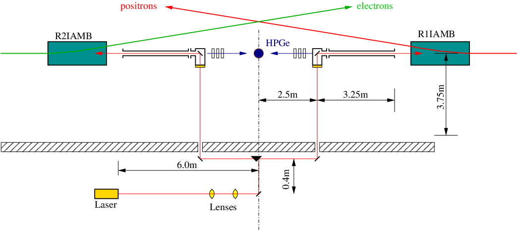
In Ref.[12] it was suggested to calibrate both and beam energies using the same HPGe detector. This approach reduce the cost of the system. The system should be placed at the opposite to the beams interaction region side of the collider. The BEPC-II beam energy calibration system layout is shown in Fig. 6 (all the lengths are approximate).
The input of the laser radiation into the BEPC-II vacuum chamber is the most complex unit of the system. The BEPC-II vacuum chamber design is shown in Fig.6. The laser beam insertion system is connected to the flange of the chamber. The distance between the vacuum chambers flanges of the electron and positron rings is equal to 11.5 m. The HPGe detector is placed between the flanges on the equal distance from both (Fig. 6).

3.1 Laser-to-vacuum insertion assembly
The conceptual scheme of laser-to-vacuum insertion system is shown in Fig.7.

The laser beam is inserted to vacuum chamber through the ZnSe or ZnS (Cleartan®) entrance window. In the vacuum chamber the laser beam is reflected on the angle 90∘ by a copper mirror, which is mounted with a good thermal contact on the massive copper support. This support can be turned by bending the vacuum flexible bellow (sylphon). So the angle between the mirror and the laser beam can be adjusted as necessary. After backscattering the photons return to the mirror, pass through it and leave the vacuum chamber. Then they can be detected by the HPGe detector. The SR radiation photons fall on the mirror and heat it. In order to reduce the heat of the mirror it is placed at the 3.25 m distance from the BEPC-II vacuum chamber flange.
| Beam energy , GeV | 2 |
| Beam current , A | 0.91 |
| Bending radius , cm | 913 |
| Mirror size , cm | 4.0 |
| Distance to mirror , cm | 605 = 280 + 325 |
| , mrad | 6.6 |
| SR power on the mirror, W | 150 |
The SR radiation power absorbed by the mirror can be estimated as follows:
| (36) |
where is the beam current, is the particle energy loss per turn due to SR radiation, . Here is the mirror size seen from the SR photons radiation point ( is the mirror width), is the distance between the mirror and the SR photons radiation point. The energy loss can be obtained using the following formula:
| (37) |
where is the beam trajectory radius in the bending magnet. Using the values of BEPC-II parameters presented in Table 1 we obtained W. The abstraction of heat outside the vacuum chamber to some cooling system is provided by the massive cooper support of the mirror.
3.2 Laser – electron beam interaction area.
The laser and / beams will interact in the straight sections of the BEPC-II, enclosed between R1IMB01 and R1IAMB dipoles for (R2IMB01 and R2IAMB for ). The lattice functions of the BEPC-II straight section are shown in Fig. 9. The electron and laser beam size in and projections versus -coordinate of the beam axis are shown in Fig. 9, 11. The laser beam is focused at the BEPC-II vacuum chamber entrance flange, where the geometrical aperture is minimal (vertical size is 14 mm). The divergence of the laser beam is defined by its transverse size at the waist, see eq.(21).
The scattered photon flux (Fig. 11) was calculated using the following formulae:
| (38) |
The total yield of photons is about 17000 ph/s/mA/W
3.3 Location of optic elements
Optic components require careful alignment and mechanical stability. It is very convenient to have a free access to them independently from the collider operation. This elements should be placed outside the BEPC-II tunnel in the neighbour hall (which is available and empty now) as shown in Fig. 6. This requires drilling a holes in the inner wall of the BEPC-II tunnel. The following optical units are situated along the collider tunnel wall:
- 1.
the mobile reflection prism which provide to change the direction of laser beam insertion (to e+ or e- beam pipe),
- 2.
the two mirrors which provides the laser beam turning on the angle 90∘. The mirrors are installed on a special supports with precise vertical and horizontal angular alignment by stepping motors (one step equals to rad).
The other optical elements: two lenses with the focal length cm and laser are placed along the neighbour wall (Fig. 6). The total distance from the laser output aperture to the entrance flange of the BEPC-II vacuum chamber is about 18.0 m. The laser beam transverse size at this flange should be equal to 0.20 – 0.25 cm (Fig.9, 11). The lenses should be placed at distance 300.0 and 381.6 cm from the laser in order to provide this size (Fig.11).


4 Conclusion
The proposed energy calibration system will provide relative accuracy in the beam energy range from 1 to 2 GeV. Some of system units are ready or in work. The goal of the further efforts should be the manufacture and purchase of the system elements and its installation at launching at BEPC-II to January 2009.
5 Acknowledgments
The authors are grateful to Fred Harris, Wolfgang Kuehn, Qian Liu, Stephen Olsen, QingBiao Wu, JianYong Zhang and QingJiang Zhang for useful discussions.
References
- [1] A.N. Skrinsky and Yu.M. Shatunov, Sov. Phys. Uspekhi 32 (1989) 548
- [2] Status of BEPCII/BESIII project. By BEPCII/BESIII Collaboration (Zhen-An Liu for the collaboration). Feb 2004. 5pp. Prepared for 9th Accelerator and Particle Physics Institute: APPI 2004, Iwate, Japan, 16-20 Feb 2004. Published in *Appi 2004, Accelerator and particle physics* 86-90
- [3] R.Klein et al., NIM A 384 (1997) 293-298, J. Synchrotron Rad. (1998) 5, 392-394
- [4] N. Muchnoi et al., in Proc. of the EPAC, Scotland, Eidenburgh, 26-30 June 2006, EPAC, 1181-1183
- [5] B.A.Shwarz for KEDR collaboration. Nucl.Phys.Proc.Suppl.169 (2007) 125-131. (e-Print: hep-ex/0611046).
- [6] M.A. Furman. The Møller Luminosity Factor. LBNL-53553, CBP Note-543. (2003)
- [7] F.R. Arutunyan, V.A. Tumanyan. Zhurnal Experimentalnoj Teorticheskoj Fiziki, vol. 44 (1963) p. 2100.
- [8] G.Ya.Kezerashvili, A.M.Milov, N.Yu.Muchnoi and A.P.Usov. A Compton Source of High Energy Polarized Tagged Gamma-Ray Beam. The ROKK-1M Facility. // Nucl. Inst. Meth. B145 (1998) p. 40-48.
- [9] Encyclopedia of Laser Physics and Technology (http://www.rp-photonics.com/gaussian_beams.html)
- [10] A. Jerrard, M. Berch. Introduction to Matrix Optics Moscow, Mir, 1978,
- [11] O.Zvelto. Printzipy Laserov. //Moskva, Mir, (1984).
- [12] Some issues of energy measurement at BESIII. IHEP, Beijing, Preliminary Study 2007.