Nonmodal energy growth and optimal perturbations in compressible plane Couette flow
Abstract
Nonmodal transient growth studies and estimation of optimal perturbations have been made for the compressible plane Couette flow with three-dimensional disturbances. The steady mean flow is characterized by a non-uniform shear-rate and a varying temperature across the wall-normal direction for an appropriate perfect gas model. The maximum amplification of perturbation energy over time, , is found to increase with increasing Reynolds number , but decreases with increasing Mach number . More specifically, the optimal energy amplification (the supremum of over both the streamwise and spanwise wavenumbers) is maximum in the incompressible limit and decreases monotonically as increases. The corresponding optimal streamwise wavenumber, , is non-zero at , increases with increasing , reaching a maximum for some value of and then decreases, eventually becoming zero at high Mach numbers. While the pure streamwise vortices are the optimal patterns at high Mach numbers (in contrast to incompressible Couette flow), the modulated streamwise vortices are the optimal patterns for low-to-moderate values of the Mach number. Unlike in incompressible shear flows, the streamwise-independent modes in the present flow do not follow the scaling law , the reasons for which are shown to be tied to the dominance of some terms (related to density and temperature fluctuations) in the linear stability operator. Based on a detailed nonmodal energy analysis, we show that the transient energy growth occurs due to the transfer of energy from the mean flow to perturbations via an inviscid algebraic instability. The decrease of transient growth with increasing Mach number is also shown to be tied to the decrease in the energy transferred from the mean flow () in the same limit. The sharp decay of the viscous eigenfunctions with increasing Mach number is responsible for the decrease of for the present mean flow.
1 Introduction
The linear stability (LS) analysis of compressible flows is of interest from the viewpoint of basic understanding on transition scenarios in such fluids [1, 2, 3], and also because of its relevance in many high speed aerodynamic design problems. Since the growth of a small disturbance can lead to the flow breakdown, an understanding of different growth mechanisms becomes more relevant. The normal mode approach, where the initial value problem is reduced to an eigenvalue problem by considering the disturbance growth/decay in terms of an exponential time dependence, has been widely studied in the past. For more than a decade, however, the traditional modal stability analysis has been complemented by the analysis of transiently growing perturbations for various shear flow configurations [4, 5, 6, 7, 8]. Such transient growth analyses have revealed that a flow can sustain large transient growth of energy in the parameter space that is stable according to the LS theory. It has been shown that the transient growth analysis can provide a possible reason for the experimentally observed critical Reynolds number () of various canonical flow configurations being less than that predicted by the LS theory (for a detailed review see the recent book of Schmid and Henningson [9]).
It is well known that there are flow configurations (e.g. the plane Couette flow, pipe flow, etc.) that are stable according to the LS theory, but have been shown to have a finite in experiments. Therefore the nonlinear effects may destabilize these flows in the stable parameter region of the LS theory. However, for the nonlinearities in the governing equations to take over, the amplitudes of the disturbances must be large. Therefore, there may be a linear mechanism that causes an infinitesimally small disturbance already present in the flow to grow initially, so that the nonlinearities could act upon them. Such a mechanism for the transient growth exists due to the nonmodal growth caused by the non-orthogonality of the LS operator [9]. In the stable region of the parameter space, even though each eigenstate decays during its evolution in space or time, a superposition of such eigenstates has potential for the transient inviscid growth before being stabilized by the viscosity at the rate of the least decaying mode. The experimental confirmation of this transition scenario comes from the observation that streaks precede the breakdown of laminar shear flows. Since the transient energy growth is maximum for streamwise vortices which subsequently give birth to streaks, it suggests that this transient growth mechanism provides a robust route to flow breakdown via disturbances that are stable according to LS theory.
Even though the transient growth analysis has been extensively studied for incompressible flows [5, 10, 6, 7, 8, 9, 11], similar studies on compressible flows are scarce [12, 13, 14, 15]. For compressible boundary layers, Hanifi, Schmid and Henningson [12] have found the maximum transient energy growth () increases with both Reynolds number () and Mach number (). They have used an energy norm such that the pressure-related energy transfer rate is equal to zero. They also cofirmed that the streamwise vortices are the optimal patterns as in incompressible flows. Farrell and Ioannou [14] have investigated the transient energy growth of 2D perturbations in the Couette flow (uniform shear flow) of a polytropic fluid with constant viscosity coefficients. They found that increases with Mach number. Recently, Tumin and Reshotko [15] have developed a ‘spatial’ model of transient growth phenomena in compressible boundary layers.
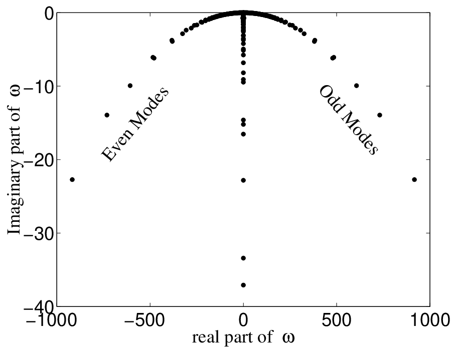
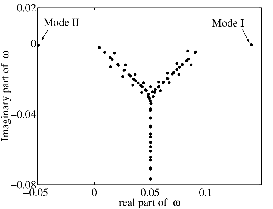
The present work deals with the ‘temporal’ stability analyses of the compressible plane Couette flow. The modal linear stability analysis of this flow has been reported by many investigators in the past [16, 17, 18]. In the incompressible limit this flow remains stable but instability is possible for a range of supersonic Mach numbers, the origin of which is tied to a family of acoustic modes [17, 18]. Duck, Erlebacher and Hussaini [17] have classified these acoustic modes into two distinct families depending on their phase speeds (see Fig. 2, the detailed description of this figure is provided in Sec. 3.1): the odd-modes (I, III, …) that have phase speeds greater than unity in the limit of zero streamwise wavenumber (), and the even-modes (II, IV, …) that have phase speeds less than zero as . (For the plane Couette flow, the non-dimensional velocities of the walls are bounded between and since the top-wall velocity has been used for non-dimensionalization, see Fig. 1.) From an asymptotic analysis of the inviscid equations, they showed that the mode-I remains neutrally stable, but the mode-II can become unstable in the inviscid limit for large . Hu and Zhong [18] studied the same viscous plane Couette flow problem numerically, and reported new viscous instabilities. In particular, they showed that the mode-I can become unstable at finite Reynolds numbers due to the effects of viscosity but the ranges of Mach numbers and wavenumbers are very narrow. They further showed that the viscosity plays a dual role of stabilizing/destabilizing the mode-II instability. The inviscid mode-II instabilty of Duck et al. that occurs at large is weakly stabilizied by viscosity, but the same mode-II is also unstable for low streamwise wavenumbers purely due to viscous effects [18]. Even though the higher-order even modes (IV,…) can also become unstable, the mode-II instablity represents the dominant instability for the compressible plane Couette flow.
In this paper, the nonmodal transient energy growth analysis is reported for the compressible plane Couette flow of an appropriate perfect gas model for three-dimensional disturbances. The governing equations and the mean flow are detailed in Sec. 2. The linear stability problem is formulated in Sec. 3, and the related numerical method and its validation are detailed in Sec. 3.1. For the tranisent growth analysis, the disturbance size is measured in terms of the Mack energy-norm [2, 3]. The results on the energy growth, the optimal perturbations and their structure, and the scalings of maximum transient growth are presented in Sec. 4. The constituent energies transferred from the mean flow, the viscous dissipation, the thermal diffusion and the shear-work during the transient growth are investigated in Sec. 5 for the initial perturbation configuration that would reach the optimal configuration at a later time. The inviscid limit of stability equations are analysed in Sec. 5.1. The conclusions are provided in Sec. 6.
2 Governing Equations
We consider the plane Couette flow of a perfect gas of density and temperature , driven by the relative motion of two parallel walls that are separated by a distance . The top wall moves with a velocity and the lower wall is stationary, with the top-wall temperature being held fixed at . Note that the quantities with a superscript are dimensional, and the subscript refers to the quantities at the top wall. The velocity field is denoted by , with , and being the velocity components in the streamwise (), wall-normal () and spanwise () directions, respectively. For non-dimensionalization, we use the separation between the two walls as the length scale, the top wall velocity, , and temperature, , as the velocity and temperature scale, respectively, and the inverse of the overall shear-rate, , as the time scale. The governing equations are the three momentum equations, continuity, energy and state equations which are omitted for the sake of brevity. The flow is described by the Reynolds number , the Prandtl number and the Mach number , defined via
| (1) |
Here is the ratio of specific heats, the thermal conductivity, and the universal gas constant; the Prandtl number is assumed to be a constant, and . For the shear viscosity , we use the Sutherland formula
| (2) |
Following Stokes’ assumption, we set the bulk viscosity to zero (i.e., ) such that
To make a direct comparison with earlier linear stability results of the compressible plane Couette flow [17, 18], we have used the same constitutive model for the transport coefficients of a perfect gas.
2.1 Mean flow
The mean flow is that of the steady, fully developed plane Couette flow for which the mean fields are given by
| (3) |
Hereafter the subscript is used to refer to the mean flow quantities. The continuity and the -momentum equations are identically satisfied for this mean flow. From the -momentum equation, it is straightforward to verify that the mean pressure, , is constant, chosen to be . Hence, from the equation of state, the mean density is related to the mean temperature via . The remaining -momentum and energy equations for the mean flow are
| (4) | |||||
| (5) |
which have to be solved, satisfying the following boundary conditions:
| (6) |
where is the non-dimensional temperature of the lower wall. The energy equation can be solved exactly to yield the temparature in terms of the flow velocity [17]:
| (7) |
where
| (8) |
is the recovery temperature, and is the temperature ratio. The streamwise velocity, , is then calculated numerically by solving the following equation:
| (9) |
using a fourth-order Runge-Kutta method. The shear stress, , is a constant that must be determined iteratively such that satisfies its boundary values:
| (10) |
With , which corresponds to an adiabatic lower wall, the calculated profiles of the mean velocity (), the temperature (), the shear rate () and the viscosity () are shown in Fig. 1 for two representative values of the Mach number, and . (Note that the mean flow profiles do not depend on Reynolds number.) Clearly, the shear-rate, the temperature and the viscosity are non-uniform along the wall-normal direction; the deviation from the corresponding uniform shear flow increases with increasing . We shall return back to discuss the effects of non-uniform mean flow on certain aspects of the transient growth results in Sec. 5.1.

3 Linear Perturbation System
We impose three-dimensional (3D) perturbations on the mean flow described in Sec. 2.1. The flow quantities with small-amplitude disturbances are considered as , where represents any mean flow quantity, and is its perturbation. For , the governing equations are linearised with respect to . Then the solutions of the linearized equations are assumed in the form of normal modes, i.e.,
| (11) | |||||
| (12) |
where and are the streamwise and spanwise wavenumbers, respectively, and is the complex frequency. The imaginary part of the complex frequency, , represents the growth/decay rate of perturbations, and its real part, , is related to the phase speed of the perturbation via . The flow is said to be asymptotically stable if , unstable if and neutrally stable if . Later for the transient growth analysis (Sec. 4), a summation over all ’s with appropriate coefficients will be implied on the right-hand-side of equation (12).
The perturbation pressure is removed from the linearized equations by using the perturbed equation of state
| (13) |
Similarly, the perturbation viscosity is written in terms of perturbation temperature:
where is evaluated at mean flow conditions. Finally, the reduced ordinary differential eigensystem in five unknowns can be written as
| (14) |
where is the eigenfunction and the identity matrix. The elements of the linear operator are given in the appendix. The boundary conditions are:
| (15) |
Note that the temperature boundary condition corresponds to an isothermal upper wall and an adiabatic lower wall as in the work of Duck et al. [17] and Hu and Zhong [18].
3.1 Numerical method and code validation
The differential eigenvalue problem (14)-(15) is discretized by using the Chebyshev spectral method [19]. The transformation is used to map the physical domain to the Chebyshev domain . The equations are collocated at the Gauss-Lobatto collocation points:
| (16) |
which are the extrema of the -order Chebyshev polynomial . There are two sub-methods of the Chebyshev spectral method to discretize this eigenvalue problem (14). In one method, any function , say, is approximated by using a Chebyshev polynomial of degree :
| (17) |
with the Chebyshev coefficients being treated as ‘unknowns’. The derivatives of are also found in terms of these polynomials through a recurrence relation that they satisfy [9]. In the other method, the function is expressed in terms of its values at the collocation points using an interpolant that uses Chebyshev polynomials, and the derivatives are found from an interpolation formula (see Malik [19] for details). This latter method is convenient since it results in a simple eigensystem, whereas the former results in a generalized eigensystem. The , , -momentum equations and the energy equation are replaced by the boundary conditions for , , and at walls, respectively. The unused -momentum equation is used to replace the continuity equation at the walls (also termed as artificial boundary condition [19]). Since the boundary conditions are independent of the eigenvalue , the right hand side of the eqn (14) would be singular, as the rows corresponding to boundary points would be zero. This singularity is removed by the row/column operations, resulting in a reduced system. The QR-algorithm of the Matlab software is used to solve this eigenvalue system.
To validate the stability code, we have compared our numerical results on asymptotic stability with the results of Hu and Zhong [18]. For example, for the parameter values of , , and with collocation points, our data on both growth rate and frequency match those of Hu and Zhong upto the fourth decimal place. For this parameter set, the distribution of eigenvalues, , is shown in Fig. 2(), and the enlargement of Fig. 2() is shown in Fig. 2() that portrays the well-known ‘Y’-branch of the spectra that belongs to viscous modes. Following the classification of Duck et al. [17], the odd-family (I, III, …) and even-family (II, IV, …) of inviscid/acoustic modes are shown in Fig. 2(); the mode-I and mode-II are indicated in Fig. 2(). Note that the ‘Y’-spectrum for compressible Couette flow becomes difficult to resolve numerically if and are large [17, 18].
|
|

|

|
Now we present a few representative stability diagrams for compressible plane Couette flow, delineating the zones of stability and instability. Figure 3() shows the contours of the growth rate of the least decaying mode, , in the -plane for two-dimensional disturbances () at a Mach number of . (This plot matches well with Fig. 20 of Hu and Zhong [18].) For 3D disturbances, Fig. 3() shows the contours of in the ()-plane for and . In each plot, the flow is unstable inside the neutral contour, denoted by ‘’, and stable outside. The mode-II (see Fig. 2) is responsible for the observed instabilities; for other details on linear stability results the reader is referred to Hu and Zhong [18].
For the transient growth analysis, we will focus on the control parameter space (such as in Fig. 3) where the flow is stable according to the modal linear stability analysis, and investigate the potential of this ‘stable’ flow to give rise to transient energy growth.
4 Transient Energy Growth
To study the evolution of a general non-eigenstate, we relax the assumption of exponential time dependence. The linear perturbation equations can be written as [9]
| (18) |
where is the inverse Fourier transform of , as given by (11). The state function is expanded in the basis of its eigenfunctions as
| (19) |
where the index runs through a selected portion of the least decaying eigenmodes in the complex eigenvalue plane (refer to Fig. 2). Using (19), the equation (18) can be diagonalized as
| (20) |
where and .
To compute the nonmodal energy growth, we need an expression for the perturbation energy. Under a suitable definition of the inner product, the square of the norm can be made to represent a measure of this energy density, . The energy density is defined as that of Mack [2, 3]
| (21) |
where the weight matrix,
| (22) |
is diagonal. In this definition of , the spatial average of the rate of pressure-related work (i.e. the compression work) is zero. As elaborated by Mack [3], the contribution of this compression work to the total perturbation energy should vanish due to the conservative nature of the compression work. Note that the Mach energy norm (21) has also been used in the ‘spatial’ transient growth analyses of compressible flows [15].
Let be the amplification of the initial energy density maximized over all possible initial conditions, i.e.,
| (23) |
For the numerical evaluation of , we refer the readers to Refs. [6, 9, 12].

|

|
A typical variation of the energy amplification factor, , with time is shown in Fig. 4(), for the parameter values of , and . There is a 200-fold increase of the initial energy density at . Since the flow is stable for this parameter combination, decays in the asymptotic limit (). To compute we do not need to consider all modes since we have found that the modes with large phase speeds (see Fig. 2) do not contribute to the energy growth. This observation is similar to the earlier findings for compressible boundary layers [12]. Therefore, to reduce the computational effort, the index in (19) is chosen corresponding to the modes whose phase speeds are within the range (i.e., comparable to the extremes of the mean flow velocity which varies between and ), and the decay rate is less than (i.e., ). With this choice of modes, the maximum possible energy amplification over time,
| (24) |
saturates to some constant value with the number of modes retained , as shown in Fig. 4(). It is observed that out of a total of modes, only modes are sufficient to compute accurately, and the contribution of the remaining modes to is negligibly small.

|
For and , the contours of in the ()-plane are shown in Fig. 5(). For other values of and , the -contours look similar. It is observed that varies non-monotonically with streamwise wavenumber for fixed , and is maximum for non-zero values of ; increases with Reynolds number for any value of . The latter observation mirrors similar findings on transient growth in incompressible fluids [9].


|
Moving onto the effect of Mach number on the transient energy growth, we show, in Fig. 6() and 6(), the contours of in the ()-plane for and , respectively; the Reynolds number is set to . It is observed that the magnitude of decreases sharply as we increase the Mach number from to for any combination of and . The supremum of over all possible combinations of wavenubers is called the optimal energy growth, :
| (25) |
which corresponds to . In Fig. 6(), this global maximum is seen to occur at and . Also, decreases by an order of magnitude with increasing Mach number as seen in Figs. 6() and 6(). (An explanation for this behaviour is provided in the next section, along with a detailed energy analysis in terms of different constituent energies.) It is worth pointing out that our result on the decrease of with is in contrast to that for boundary layers [12].


|
The variations of the optimal growth , the corresponding optimal time , the optimal streamwise, , and transverse, , wavenumbers with the Mach number are shown in Fig. 7(-); as in Fig. 6, for these plots. It is observed that while both and decrease monotonically with increasing , both the optimal wavenumbers ( and ) vary nonmonotonically in the same limit. (Note that the wiggles in panels and are due to the searching of in the ()-plane with small but finite grid-spacing– these computations are very time consuming.) Figure 7() shows the interesting result that the optimal streamwise wavenumber can become zero at large . This is in contrast to the incompressible Couette flow for which stays always slightly away from the null value [9].
4.1 Structure of optimal disturbances
The initial disturbance pattern for given values of and that reaches the maximum possible transient growth at along with the corresponding disturbance pattern at time can be determined through the singular value decomposition [9]. In the following, such disturbances at and are referred to as the optimal disturbances.

Before presenting the structure of optimal velocity patterns, we show the variation of with time, denoted by the dash line, in Fig. 8 for the particular initial perturbation that reaches maximum energy, , at a time . The parameter values are set to , , and . For comparison, we have also superimposed the variation of with time, denoted by the solid line. As expected, the envelope of is below that of since the former corresponds to a particular initial condition but the latter to all possible combinations of initial conditions that yields maximum amplification at any time.

|

|

|
For the maximum energy growth as in Fig. 8, the optimal velocity patterns at and in the -plane are shown in Fig. 9() and Fig. 9(), respectively. (Note that these patterns are invariant along the streamwise direction since .) Both patterns resemble streamwise vortices which are typical of all shear flows. It is noteworthy that the optimal pattern in Fig. 9() has two counter-rotating streamwise vortices along the wall-normal direction. The inviscid rapid growth of these optimal patterns for null or very low values of the streamwise wavenumber () is due to the lift-up mechanism [20] during the motion of the fluid particles in the wall-normal direction. Another typical feature of shear flows is the spanwise alternating streamwise velocities as shown in Fig. 9().

|

|
Figures 10() and 10() show representative two-dimensional () optimal velocity patterns in the plane. The parameter values are set to , and . It is observed that the pattern at has structures that locally oppose the mean shear. This pattern subsequently evolves into two ‘cross-flow’ vortices at . This final configuration is the outcome of the well-known Orr-mechanism [4] that leads to transient energy growth due to the tilting of the initial perturbations into the direction of the mean shear as time evolves.


|


|
Returning to the variation of the optimal wavenumber, , with the Mach number in Fig. 7(), we note that is very small but finite at low-to-moderate values of and zero at some large value of . This implies that the pure streamwise vortices are the optimal patterns at high Mach numbers, but their modulated cousins are the optimal patterns for low-to-moderate values of the Mach number. Our results on optimal patterns at high Mach numbers () should be contrasted with that for incompressible Couette flow for which the oblique modes constitute optimal patterns. Typical optimal patterns of such modulated streamwise vortices are shown in the - and -plane in Fig. 11 for the optimal energy growth () at , with other parameters as in Fig. 7. We conclude that the structural features of the optimal disturbance patterns in compressible Couette flow look similar to those of incompressible shear flows.
4.2 Scalings of and
For incompressible channel flows with streamwise-independent modes (i.e., ), Gustavsson [10] has shown that varies quadratically with the Reynolds number , and varies linearly with . More specifically, when the energy growth curve, such as the one in Fig. 4(), is plotted in terms of and , the renormalized growth curves for different collapse onto a single ‘universal’ curve. Following a similar analysis, Hanifi and Henningson [13] found that this scaling law also holds for compressible boundary layers. However, for the present Couette flow of non-uniform shear and non-isothermal fluid, this scaling law does not hold as shown in Fig. 12 which displays plots of verses for a wide range of at . Similar trends persist at other values of Mach number (not shown for brevity).

|

|
For the present flow configuration, it can be verified that the Mack transformation [3, 13]
| (26) |
(hence , from the equation of state), can make the streamwise-independent linearized stability equation (18) independent of the Reynolds number , except for the terms associated with density and temperature fluctuations in the - and -momentum equations (i.e., and as detailed in the Appendix). Only on neglecting these terms, one can show that as detailed by Hanifi and Henningson [13] who further assumed that to neglect and for large . The above pressure-related terms may not be negligible for all mean flows. This can be ascertained for the present flow configuration if we recompute the energy growth by setting
| (27) |
in the linear operator . Indeed the rescaled growth curves for different Re now collapse onto a single curve as shown in Figs. 13(-), for the same parameter values as in Figs. 12(-). (Note that in these plots the energy growth does not decay since the above procedure (27) introduces some ‘artificial’ neutral modes in , resulting in an asymptotic value for at large times.) Therefore, we conclude that the non-negligible values of and for the plane Couette flow are responsible for the invalidity of the scaling law .

|

|
We note in passing that Hanifi and Henningson’s [13] assumption of leads to a change in the equation of state by introducing a factor of into it. The form-invariance of the equation of state is essential since it has been used to remove from the linear perturbation system. In general, the (streamwise-independent) linear operator of compressible flows cannot be made free from the apearance of (via the Mack transformation), and hence the scaling, , would not hold for all mean flows. For special cases, the terms and might be negligible (e.g. in compressible boundary layers [13] at high ) and hence the scaling law would hold there.
5 Nonmodal Energy Budget
We now consider the evolution equation for the perturbation energy . Multiplying (18) by and adding the complex conjugate of the resulting equation to itself, we obtain the evolution equation for as
| (28) |
with being the complex-conjugate term. In the above equation, the total perturbation energy has been decomposed into several constituent energies, :
| (29) | |||||
| (30) | |||||
| (31) | |||||
| (32) | |||||
Here, represents the energy transfer from the mean flow, is the viscous dissipation, the thermal diffusion and the shear-work, respectively. Note that there is an additional term, ,
| (33) | |||||
representing the convective transfer of perturbation energy (by the mean flow), which is identically zero. The decomposition of the total perturbation energy into different constituents, as in (29-32), is useful to analyse the role of each constituent energy on the growth/decay of total energy. The evolution equation (28) provides an energy-budget for the total perturbation energy, and helps to quantify the contributions of different kinds of perturbation energies, leading to the transient growth.
To analyse the nonmodal energy budget, we choose a set of values for , , and that leads to transient growth. The constituent energies, , are then each evaluated using a quadrature formula with an initial perturbation configuration that would reach the optimal energy. The initial values of the constituent energies are chosen as so that the total intitial energy is equal to the normalized value.

|

|
Figure 14() shows the energy budget for three-dimensional disturbances with ; other parameters are as in Fig. 4(). For this case, the energy gain by the shear-work term, , is found to be negligible and hence not shown in this plot. It is observed that the energy transferred from the mean flow, , (denoted by the dash line) increases with time, reaching a large asymptotic value beyond the optimal time (); this is the major cause for the transient growth. At some later time (), this transient growth is nullified by the energy taken away by the thermal diffusion, , (denoted by the line with solid symbols) and the viscous dissipation, (dot-dash line). For this parameter set, the energy loss due to the viscous dissipation dominates over that due to the thermal diffusion at large times.
Figure 14() shows the same energy budget for a representative case of streamwise independent () disturbances, with parameter values as in Fig. 8. As in the previous case (Fig. 14), the energy transferred from the mean flow is responsible for the transient growth; however, unlike in Fig. 14(), reaches a peak and then decreases to attain an asymptotic value. The variations of the other constituent energies are similar to those in Fig. 14().

|

|
In the previous section, we found that the optimal transient energy growth decreases with increasing Mach number. To explain this behaviour in terms of constituent energies, we show the energy budget versus Mach number in Fig. 15 for the optimal values of (as in Fig. 7). Note that the total energy curve shown in Fig. 15() (denoted by the solid line) matches with the one in Fig. 7(). It is observed that the energy transferred from the mean flow () and the viscous dissipation loss () are the most significant compared to the other components ( and , see Fig. 15) of the perturbation energy. Since decreases with increasing , so does the total energy at the optimal time. In general, the decrease in the transient energy growth with increasing is primarily due to the decrease of the energy transfer from the mean flow to perturbations in the same limit.
For the present flow configuration, it is still not clear why the transferred energy from the mean flow, , decreases with increasing Mach number; an inviscid energy analysis provides an answer for this as well as for the transient growth mechanism.
5.1 Inviscid limit: Mechanism for transient growth
For streamwise independent disturbances (), Hanifi and Henningson [13] have shown that the inviscid linear stability equations of compressible fluids have the following solution
| (34) |
where
| (35) |
and the subscript, ‘ivs’ stands for ‘inviscid’. The nonzero elements of the matrix, , are , and . In fact, this inviscid solution for velocity perturbations is the same as that of Ellingsen and Palm’s incompressible solution [21]. The inviscid perturbation energy, , maximized over , in the same definition of the energy norm, is given by
| (36) |
where ’s are the eigenvalues of the differential equation
| (37) |
with being the associated linear differential operator
| (38) |
The above equation is solved using the same spectral method described in Sec. 3.1 with the following boundary conditions:
| (39) |

|
Figure 16 shows the variation of with time for and . For comparison, the viscous -curves at various are also displayed. In terms of different energy components, the inviscid energy growth rate of the optimal perturbation configuration is given by (29), since the transfer rates of the other energy components, and are zero in the inviscid limit. Therefore the reason for the inviscid growth is due to the energy transferred from the mean flow to perturbations, i.e. . This energy transfer occurs due to an algebraic instability [20, 21], wherein the streamwise perturbation velocity, density and temperature grow algebraically (linearly) with time. if the initial normal perturbation velocity is non-zero (i.e. ). A noteworthy point in Fig. 16 that the inviscid growth-curve, , coincides with the viscous curves only for a very short time– we shall return to explain this point later. Note that this observation is in contrast to boundary layers (see Figs. 1 and 2 in ref. [13]) for which the viscous growth curves (at different ) closely follow the inviscid growth-curve till they achieve their maxima .
The inset in Fig. 16 shows the curves of () for three different Mach numbers. Clearly, at any time, increases with increasing for the inviscid case. This is in contrast to the viscous case where we have seen a steady decrease of with increasing (dashed line in Fig. 15). To understand this difference, let us rewrite the energy transfer rate (29) as
| (40) |
which is identical for both the inviscid and viscous cases. Now combining (40) with (34), we obtain
| (41) |
In this equation the -dependence is present only via . Note that the inviscid temperature eigenfunction,
| (42) |
grows quadratically with since . It can be verified that the dominant contribution to in (41) at large comes from the energy associated with temperature fluctuations, and hence, for any given initial condition, the norm of would increase with increasing . We can conclude that the increase of the inviscid energy growth with increasing is primarily due to the increased energy transfer from the mean flow to temperature fluctuations.
Though the above contribution is also present for the viscous case, the decay of the viscous eigenfunction by viscosity becomes dominant with increasing as we show below. Compared to the inviscid eigenfunction , the viscous eigenfunction decays due to viscous dissipation and thermal diffusion (both of which involve viscosity ). Under the assumed viscosity-law (2), the viscosity of the mean flow increases rapidly with increasing Mach number at all points in the normal direction (see Fig. 1), resulting in a decrease in the viscous eigenfunction in the same limit. To quantify the last statement, we calculate the following for the viscous problem:
| (43) |
which is a measure of the collective evolution (growth/decay) of all eigenfunctions. Here, the summation index runs over the perturbation velocity, density and temperature, and the index runs over the selected eigenmodes (see eqn. 19); stands for the imaginary part, and stands for the trace of the matrix. The initial condition, , is chosen as . It should be pointed out that the measure for the collective growth/decay of eigenfunctions, via (43), is equivalent to probing the energy-norm with an unit weight matrix . Our definition simply masks out the Mach-number dependence of the energy norm due to the base-state variables in (as in the Mack energy norm).

.
Figure 17 shows the variation of with time for two Mach numbers; other parameters are and . It is clear from this figure that the (collective) decay-rate of eigenfunctions at any time is higher for higher Mach number. Therefore, the viscous eigenfunctions are small at a time or and at a Mach number in comparison with that at any lower value of the Mach number , leading to a decrease in the energy transfer from the mean flow to perturbations with increasing Mach number. This decay can only come from the dependence of the viscous eigenfunctions on the shear viscosity (which increases with increasing ). In contrast, the inviscid eigenfunctions grow with as we have pointed out earlier. Therefore, the difference in the variation of with for the inviscid and viscous cases stems from the different variations of the respective eigenfunctions with .
The reason for the viscous growth curves (in Fig. 16) not coinciding with the inviscid curve during the most part of the transient growth can be related to the fact that the viscous eigenfunctions undergo sharp decays with time for the present mean flow. (Note that the non-dimensional viscosity takes a value that is always greater than one in the entire domain, see Fig. 1.) Here, the viscous-decay of eigenfunctions with time (as in Fig. 17) competes with the inviscid growth of eigenfunctions. Clearly, the decay of with time is not negligible compared to the algebraic growth even duing the initial times, and this decrease becomes more and more important at later times. Hence, the -curves for various do not coincides with their inviscid counterpart .
Returning to the compressible boundary layers [13], we had noted that the viscous growth curves, , coincide with the inviscid curve till they achieve their maxima . A plausible explanation for this could be that the temperature, and hence the viscosity, for boundary layers remains constant for more than of the domain (since the variations of mean-fields are concentrated within a few displacement thickness while the mean flow extends upto a few hundred times of the displacement thickness). Therefore, the viscous-decay of , compared to the inviscid (algebraic) growth, may not be as strong in boundary layers as in the present mean flow. This issue needs further investigation.
6 Summary and Conclusion
We have investigated the nonmodal transient growth characteristics and the related patterns in compressible plane Couette flow of a perfect gas with temperature-dependent viscosity. The mean flow consists of a non-uniform shear-field and varying temperature and viscosity along the wall-normal direction. For the transient growth analysis, the disturbance size was measured in terms of the Mack energy norm [2, 3] for which the pressure-related energy transfers are zero. The results were presented for ranges of Mach number (), Reynolds number () and wavenumbers ( and ) for which the flow is asymptotically stable.
The maximum transient energy growth, , is found to increase with increasing Reynolds number, as in many incompressible flows, but decreases with increasing Mach number. The optimal energy growth, , (i.e. the global maximum of in the -plane for given and ) decreases with increasing . This result is in contrast to that for compressible boundary layers [12] for which increases with increasing . The optimal streamwise wavenumber, , is close to zero (but finite) at , increases with increasing and reaches a maximum value at some value of , and decreases thereafter. Unlike in incompressible Couette flow [5, 9], becomes zero at large enough value of . The optimal spanwise wavenumber, , also varies non-monotonically with : decreases first and then increases with increasing . Optimal velocity patterns (at ) correspond to pure streamwise vortices for large , but the modulated streamwise vortices are optimal patterns for low-to-moderate values of . Our result on optimal patterns at very high Mach number should be contrasted with that for the incompressible Couette flow for which the oblique modes constitute the optimal patterns.
For the streamwise independent disturbances (), we have found that the transient energy growth does not follow the well-known scaling laws, and , of incompressible shear flows [10, 9]. In contrast, however, these scaling laws are known to hold for compressible boundary layers [12]. We showed that the invalidity of these scaling laws for the present flow configuration is tied to the ‘dominance’ of some terms (related to density and temperature fluctuations in the and -momentum equations) in the linear stability operator. More specifically, we found that the well-known Mack transformation (eqn. 26) does not make the streamwise-independent stability equations independent of the Reynolds number because of the above mentioned dominant terms.
An evolution equation for the perturbation energy has been derived, and various constituent energies, that are transferred to perturbations through different physical processes, have been identified. We have carried out a detailed nonmodal energy analysis for initial perturbations that yield maximum energy growth at a later time. Based on this energy budget analysis, we found that the transient energy growth occurs due to the transfer of energy from the mean flow to perturbations via an inviscid algebraic instability. We further showed that the decrease of transient growth with increasing Mach number is tied to the decrease in the energy transferred from the mean flow () in the same limit. Lastly, considering the inviscid limit of stability equations, we found that the viscous growth curves follow the inviscid growth curve () only for a very short time. This is due to the strong dependence of viscosity on Mach number for the present mean flow, resulting in sharp decays of the viscous eigenfunctions with increasing Mach number which is responsible for the decrease of in the same limit.
References
- [1] L. Lees and C. C. Lin, “Investigation of the stability of the laminar boundary layer in a compressible fluid,” NACA Tech. Note 1115 (1946).
- [2] L. M. Mack, “Boundary-layer stability theory,” JPL Rep. 900-277 (1969).
- [3] L. M. Mack, “Boundary-layer linear stability theory,” AGARD Rep. 709, 3-1 (1984).
- [4] W. M. F. Orr, “The stability or instability of steady motions of a perfect liquid and a viscous liquid,” Proc. R. Ir. Acad., A 27, 9 (1907).
- [5] K. M. Butler and B. F. Farrell, “Three-dimensional optimal perturbations in viscous shear flow,” Phys. Fluids 4, 1637 (1992).
- [6] S. C. Reddy and D. S. Henningson, “Energy growth in viscous channel flows,” J. Fluid Mech. 252, 209 (1993).
- [7] L. N. Trefethen, A. E. Trefethen, S. C. Reddy and T. A. Driscoll, “Hydrodynamic stability without eigenvalues,” Science 261, 578 (1993).
- [8] F. Waleffe, “Transition in shear flows. Nonlinear normality versus nonnormal linearity,” Phys. Fluids 7, 3060 (1995).
- [9] P. J. Schmid and D. S. Henningson, Stability and Transition in Shear Flows. (Springer-Verlag, Berlin, 2001).
- [10] L. H. Gustavsson, “Energy growth of three-dimensional disturbances in plane Poiseuille flow,” J. Fluid Mech. 224, 241 (1991).
- [11] J. Kim and J. Lim, “A linear process in wall-bounded turbulent shear flows,” Phys. Fluids 12, 1885 (2000).
- [12] A. Hanifi, P. J. Schmid and D. S. Henningson, “Transient growth in compressible boundary layer flow,” Phys. Fluids 8, 826 (1996).
- [13] A. Hanifi and D. S. Henningson, “The compressible inviscid algebraic instability for streamwise independent disturbances,” Phys. Fluids 10, 1784 (1998).
- [14] B. F. Farrell and P. J. Ioannou, “Transient and asymptotic growth of two-dimensional perturbations in viscous compressible shear flow,” Phys. Fluids 12, 3021 (2000).
- [15] A. Tumin and E. Reshotko, “Optimal disturbances in compressible boundary layers,” AIAA 41, 2357 (2003).
- [16] W. Glatzel, “The linear stability of viscous compressible plane Couette flow,” J. Fluid Mech. 202, 515 (1989).
- [17] P. W. Duck, G. Erlebacher and M. Y. Hussaini, “On the linear stability of compressible Couette flow,” J. Fluid Mech. 258, 131 (1994).
- [18] S. Hu and X. Zhong, “Linear stability of viscous supersonic plane Couette flow,” Phys. Fluids 10, 709 (1998).
- [19] M. R. Malik, “Numerical methods for hypersonic boundary layer stability,” J. Comp. Phys. 86, 76 (1990).
- [20] M. T. Landahl, “A note on an algebraic instability of inviscid instability of inviscid parallel shear flows,” J. Fluid Mech. 98, 243 (1980).
- [21] T. Ellingsen and E. Palm, “Stability of linear flow,” Phys. Fluids 18, 487 (1975).