The transition from adiabatic inspiral to geodesic plunge for a compact object around a massive Kerr black hole: Generic orbits

The following system of first order equations describes geodesics in a Kerr [11, 12] geometry:

The potentials can be expressed as:

The parameters $(r,\theta,\phi,t)$ are the Boyer-Lindquist coordinates, $M$ is the black hole mass, $\mu$ is the perturbing mass, $\Sigma=r^{2}+a^{2}\cos^{2}\theta$, $\Delta=r^{2}-2Mr+a^{2}$ and $a$ is the spin parameter of the black hole. The constants $(E,L_{z},Q)$ represent the actual energy, momentum and Carter constant (in units of $M$, $M^{2}$ and $M^{4}$ respectively), not the dimensionless versions of them. By introducing the perturbing mass explicitly, our notation deviates from previous literature. We do this in order to show the dependence of the transition phase on the mass of the perturbing object. We also set $G=c=1$ everywhere.

A standard but not unique definition of the “inclination” of a Kerr geodesic is given by

It is possible to use $\iota$ to eliminate the Carter constant. Thus, any circular orbit can be parametrized by its radius ($r$) and inclination ($\iota$).

The last stable orbit (LSO) serves as an important reference point — the inspiral is adiabatic well before the compact object crosses the LSO and is approximately a plunge well after the crossing. Since the transition occurs in the vicinity of the LSO, a preliminary step in our computation is to determine $r$ and $(E,L_{z},Q)$ at the LSO for a given inclination at the LSO, $\iota_{\rm LSO}$. Note that $\iota$ changes with time because it is a function of $[E(t),L_{z}(t),Q(t)]$.

Circular orbits satisfy

We must have $R^{\prime}=0$ because the LSO lies at an extremum of $R$. We also require that

for the extremum to be stable. This implies that the orbit will be marginally stable if $R^{\prime\prime}=0$. Thus, the three equations $R=R^{\prime}=R^{\prime\prime}=0$ can be numerically solved for a given $\iota_{\rm LSO}$ to yield $r$, $E$, $L_{z}$ and $Q$ at the LSO.

We need a model of the phase space trajectory, $[E(t),L_{z}(t),Q(t)]$ near the LSO in order to compute the world line of the compact object as it transitions from inspiral to plunge. To this end, we Taylor expand about the LSO to obtain

which are natural generalizations of equations (3.4) and (3.5) of Ref. [2]. The overdot denotes differentiation with respect to $t$. We will later see that our initial condition for $t$ amounts to choosing $t_{\rm LSO}$, the instant at which the compact object crosses the LSO. This choice is consistent with the procedure in Ref. [2] — Eq. (3.14) of Ref. [2] implies a choice of $t_{\rm LSO}=0$.

The constant terms in Eq. (16), $\delta Q$ and $\delta\dot{Q}$, are needed to guarantee that the trajectory remains circular as we enter the transition. As the notation suggests, these constants are small compared to $Q_{\rm LSO}$ and $\dot{Q}_{\rm LSO}$. They are discussed in more detail when we discuss initial conditions for the transition in Sec. II.6.

The expressions (14), (15) and (16) do not include conservative effects of the self force. Pound and Poisson [10] have demonstrated that this omission will lead to observationally significant changes. Inclusion of these effects would effectively alter the potentials, Eq. (5) - Eq. (8) leading to slight deviations of $(E,L_{z},Q)_{\rm LSO}$ and $r_{\rm LSO}$ (for a given $\iota_{\rm LSO}$) from their geodesic values. The exact impact of these effects will not be known until we know what the corrections are. We will later see that our results posses all the expected qualitative features despite this handicap. Moreover, the prescription in [2] and its generalization presented here can easily incorporate these effects once they are known.

The fluxes at the LSO remain a parameter in our code. We use the code developed in [5] to provide us the dimensionless fluxes, $(M/\mu)^{2}\dot{E}$, $(M/\mu^{2})\dot{L}_{z}$ and $(1/\mu^{3})\dot{Q}$ at the LSO. Equivalently, we can use the expressions in [13] (with zero eccentricity) for the dimensionless fluxes.

Numerical integration of the $\theta$-equation warrants some care. The issue arises because $d\theta/dt$ vanishes at the turning points, $\theta_{\rm max}$ and $\theta_{\rm min}$, where

The potential problems posed by the turning points can be eliminated by reparametrizing $\theta$. Following Ref. [5], we use

where

and $\beta=a^{2}(\mu^{2}-E^{2})/\mu^{2}$. The $\theta$-equation of motion now becomes

where

Equation (20) can now be integrated without turning points because $\chi$ varies from $0$ to $\pi$ to $2\pi$ as $\theta$ varies from $\theta_{\rm min}$ to $\theta_{\rm max}$ and back to $\theta_{\rm min}$.

In keeping with our main objective of obtaining the world line $[r(t),\theta(t),\phi(t)]$ through the transition regime, we eliminate $\tau$ by dividing equation (1) by (4) and squaring the result to obtain

One more time derivative gives the acceleration:

Ideally, Eq. (23) must have other additive terms proportional to non-zero powers of $\mu$. This is analogous to Eq. (3.10) of [2]. Excluding this term amounts to ignoring the conservative self force.

Since the transition phase is in the proximity of the LSO, we can Taylor expand $F$ about $r_{\rm LSO}$, $E_{\rm LSO}$, $L_{z,\rm LSO}$ and $Q_{\rm LSO}$ to obtain

Thus, the acceleration now becomes ¹¹ 1 Note that Eq. (24) ignores terms of order $(\mu/M)^{2}$ and higher.:

We have not expanded the second term in Eq. (23) because we do not know the value of $\chi$ at $r=r_{\rm LSO}$ a priori. Similarly, the $\phi$-equation takes the form

The trajectory in the transition phase can now be computed by integrating equations (25), (26) and (20) from some starting point outside the LSO to some ending point inside the LSO, for a given $\iota_{\rm LSO}$, with time varying $E$, $L_{z}$ and $Q$.

The angles, $\phi$ and $\chi$ can be set to zero without loss of generality. Setting $\chi=0$ corresponds to starting the inspiral at $\theta=\theta_{\rm min}$.

The choice of initial radius depends explicitly on $\mu$. In Ref. [2], the authors define parameters, $\alpha$, $\beta$, $\kappa$, $\tau_{0}$ and $R_{0}$. These are used to scale out the perturbing mass from the equation of motion and initial conditions. Although we prefer to retain dimensions in the equations of motion, we specify initial conditions in a dimensionless form, independent of $\mu$. This will be useful be in interpreting our results and making comparisons with Ref. [2]. Following Ref. [2], we define

where

with $\tilde{r}=r/M$, $\tilde{t}=t/M$, $\tilde{E}=E/\mu$, $\tilde{L}_{z}=L_{z}/(\mu M)$ and $\tilde{Q}=Q/(\mu M)^{2}$.

These definitions reduce to those presented in Ref. [2] when $\iota=0$. It is useful to observe that $\kappa$ does not scale with $\mu$. We evaluate $d\tau/dt$, $\alpha$, $\beta$ and $\kappa_{0}$ at $\theta=\pi/2-\iota_{\rm LSO}$ because we do not know $\theta_{\rm LSO}$ a priori. Notice that $X$ and $T$ are dimensionless.

The smoothness of the transition implies that there is no fixed instant at which the transition starts or ends. Motivated by the choices in Ref. [2], we set $T\simeq-1$ at $t=0$ and stop the numerical integrator when $X\leq X_{e}=-5$.

In summary, our initial conditions are $T=-1$, $\phi=0$ and $\chi=0$ at $t=0$ ²² 2 It is important to keep $|T|$ small enough that our Taylor expansion about the LSO remains a valid approximation.. Setting $T=-1$ at $t=0$ allows us to calculate $t_{\rm LSO}$ and hence $E(0)$ and $L_{z}(0)$ from equations (14) and (15). We then solve $R(E,L_{z},Q,r)=0$ and $dR/dr=0$ to obtain $r(0)$ and $Q(0)$. This is analogous to Sec. IIIC of Ref. [2] where they enforce $X=\sqrt{-T}$ to determine $X$ at $t=0$.

The trajectory is adiabatic before the start of the transition. At $t=0$, we must impose the condition [14, 15, 16] that circular orbits remain circular even under adiabatic radiation reaction. Thus, requiring that $\dot{R}=dR/dt=0$ and $\dot{R}^{\prime}=d^{2}R/drdt=0$ leads to expressions (3.5) and (3.6) of [5] for $\dot{r}(0)$ and $\dot{Q}(0)$ respectively.

We can now substitute $Q(0)$ and $\dot{Q}(0)$ in Eq. (16) to obtain two independent equations,

which can be used to evaluate $\delta Q$ and $\dot{\delta Q}$.

The previous sections developed the steps required to calculate the compact body’s trajectory as it transitions from inspiral to plunge. We now summarize the algorithm that was actually used to implement this prescription:
(1) Take $\iota_{\rm LSO}$ as input.
(2) Compute $E$ and $L_{z}$ at the LSO.
(3) Obtain $\dot{E}$ and $\dot{L}_{z}$ at the LSO from the code developed in [5]. We may also use the expressions in [13] (which reduce to the results in [5] for circular orbits), which will be particularly useful when we generalize to eccentric orbits.
(4) Choose initial conditions $T\simeq-1$, $\phi=0$ and $\chi=0$ at $t=0$.
(5) Calculate $E(0)$ and $L_{z}(0)$ from equations (14) and (15).
(6) Solve for $r(0)$ and $Q(0)$ by imposing $R=0$ and $dR/dr=0$ at $t=0$.
(7) Compute $\dot{r}(0)$ and $\dot{Q}(0)$ from equations (3.5) and (3.6) of [5].
(8) Substitute $Q(0)$ and $\dot{Q}(0)$ in Eq. (16) to evaluate $\delta Q$ and $\delta\dot{Q}$.
(9) Use a Runge-Kutta integrator on (25), (26) and (20) to compute the coordinates at the next step. A time step of $\delta t\simeq 0.05M$ works well.
(10) Update the “constants”, $E_{i+1}=E_{i}+\dot{E}\delta t$, $L_{z,i+1}=L_{z,i}+\dot{L}_{z}\delta t$ and $Q_{i+1}=Q_{i}+(\dot{Q}+\dot{\delta Q})\delta t$. The subscript $i$ denotes a discrete time instant.
(11) Repeat steps (9)-(11) until $X(t)\simeq-5$.

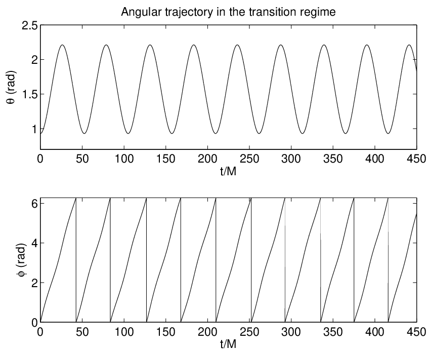
The primary objective of this calculation is to compute the world line of the compact object during the transition. Figures 1 and 2 illustrate $r$, $\theta$ and $\phi$ motions of the compact object for a typical set of parameters. We also show a plunging geodesic matched to the end of the transition.

Table 1 shows the parameters and transit times for a range of inclination angles. In general, we find that the transit time increases with inclination. However, the dimensionless transit time $\Delta T$ remains approximately constant,

when $X_{e}=-5$ for all values of $a$ and $\iota$. Again, this is a consistent generalization of the result in Ref. [2] where they find $\Delta T\simeq 3.3$ for all circular, equatorial orbits.

The results in Ref. [2] provide an important sanity check for the case of circular, equatorial orbits. However, we have to account for the minor differences between the two approaches. Ref. [2] makes the approximations

which lead to

which is a dimensionless constant. In our prescription, $d\tau/dt$ varies with time. This time dependence has to be enforced because $d\tau/dt$ is a function of $\theta$, whose value at the LSO is not known a priori. The circular, equatorial case in Ref. [2] does not suffer from this pathology because $\theta=\pi/2$ at all times. Thus, we treat $\kappa$ as a slowly varying function of time. Table 2 shows the transit times for a nearly equatorial orbit ($\iota_{\rm LSO}=0.001$) and a range of mass ratios. As the mass ratio becomes smaller, the variation in $\kappa$ decreases, and the dimensionless transit time converges to the limit where $\kappa$ is constant.

Our initial conditions differ slightly from those used in Ref. [2]. Effectively, they use the Taylor expansion of $R(r)$ to solve $dR/dr=0$ and $d^{2}R/(drdt)=0$ for $r(0)$ and $\dot{r}(0)$ respectively. In contrast, we solve the equations exactly. This leads to differences of less than $1\%$.

As with circular orbits, the last stable bound geodesic is an important reference in our procedure. The inner and outer turning points ($r_{\rm min}$ and $r_{\rm max}$) of the LSO are related to $e_{\rm LSO}$ and $p_{\rm LSO}$ through

Our goal is to determine $p_{\rm LSO}$ and the constants $(E,L_{z},Q)$ at the LSO for a given $\iota_{\rm LSO}$ and $e_{\rm LSO}$. This can be achieved by requiring that

Recall that the function $R$ is given by Eq. (5) and $\iota$ is defined by Eq. (9). We require Eq. (44) to be satisfied because the inner most turning point corresponds to a local maximum of $(-R)$. Equation (45) enforces the compact object’s velocity to vanish at the turning points. Equations (44), (45) and (9) can be solved numerically for $p$ and $(E,L_{z},Q)$ at the LSO. Appendix A describes the details of this numerical procedure.

As with the circular case, our initial conditions are such that we effectively choose the LSO crossing to occur at $t=t_{\rm LSO}$. This allows us to expand the constants about the LSO to obtain

Notice that we no longer need the corrections, $\delta Q$ and $\dot{\delta Q}$ because there are no additional symmetries to constrain $Q(0)$ and $\dot{Q}(0)$ ; $E(t)$, $L_{z}(t)$ and $Q(t)$ are independent.

As discussed in Sec. II.3, equations (46), (47) and (48) do not include conservative effects of the self force. Just as the circular case, this will lead to a slight shift of $(E,L_{z},Q)_{\rm LSO}$ and $p_{\rm LSO}$ (for a given $e_{\rm LSO}$ and $\iota_{\rm LSO}$) with respect to their geodesic values. Again, our motivation to stick with this approximation stems from the facts that: (a) These effects can be incorporated into our prescription once they are known, and (b) Our results show the generally expected behavior, at least qualitatively.

Numerical methods to calculate the change in the Carter constant due to gravitational-wave backreaction have recently become available [17, 18]. Work is in progress implementing that result in the code we use to compute the rate of change of orbital constants [19]. For now, we use the approximate expressions for $\dot{Q}$ described in [13]; it will be a simple matter to update our code when more accurate $\dot{Q}$ results are available.

Our next task is to derive equations of motion to map the phase space trajectory to an actual world line. The angular equations, Eq. (20) and Eq. (26), remain unaffected. Our strategy for the radial equation is to expand the geodesic equation about $(E_{\rm LSO},L_{z,\rm LSO},Q_{\rm LSO})$. This leaves us with

Note that we only expand about the constants, not the $r$-coordinate, because there is no unique $r$ at the LSO. In the absence of the first three terms in Eq. (50), the equation of motion is simply a geodesic at the LSO. This is consistent with our intuitive notion of “expanding about the LSO”. The existence of turning points presents a complication while integrating Eq. (50) numerically. We present a method to tackle this in Appendix B.

We need initial conditions for $r$ and $dr/dt$ before we start the numerical integrator. Motivated by the initial conditions for circular orbits, we set $T\simeq-1$ at $t=0$. This amounts to choosing $t_{\rm LSO}$. We can now determine $[E(0),L_{z}(0),Q(0)]$, which can be mapped to $(p,e,\iota)$ at $t=0$. This mapping is allowed because the trajectory is adiabatic before $t=0$. The coordinates at any point on the geodesic defined by $[E(0),L_{z}(0),Q(0)]$ can serve as our initial conditions. For simplicity, we choose

The equations of motion can now be easily integrated across the LSO.

Taking eccentricity into account changes our algorithm slightly. We summarize the code’s algorithm as follows:
(1) Take $\iota_{\rm LSO}$ and $e_{\rm LSO}$ as input.
(2) Compute $E$, $L_{z}$ and $Q$ at the LSO.
(3) Obtain $\dot{E}$, $\dot{L}_{z}$ and $\dot{Q}$ at the LSO from the expressions in Ref. [13].
(4) Choose initial conditions $T\simeq-1$, $\phi=0$ and $\chi=0$ at $t=0$.
(5) Calculate $E(0)$, $L_{z}(0)$ and $Q(0)$ from equations (46), (47) and (48).
(6) Map $\left[E(0),L_{z}(0),Q(0)\right]$ to $(p,e,\iota)$.
(7) Set $r=p/(1+e)$ and $dr/dt=0$ at $t=0$.
(8) Use a Runge-Kutta integrator on (49), (26) and (20) to compute the coordinates at the next step. A time step of $\delta t\simeq 0.05M$ works well.
(10) Update the “constants”, $E_{i+1}=E_{i}+\dot{E}_{\rm LSO}\delta t$, $L_{z,i+1}=L_{z,i}+\dot{L}_{z,\rm LSO}\delta t$ and $Q_{i+1}=Q_{i}+\dot{Q}_{\rm LSO}\delta t$. The subscript $i$ refers to a discrete time instant.
(11) Repeat steps (9)-(11) until $X\simeq-5$.

Recall that the local minimum of the potential $R$ is less than zero for bound orbits and is greater than zero for a plunging geodesic. The minimum is exactly zero at the LSO. These conditions can be used as sanity checks while performing the numerical integration.

Figures 3, 4 and 5 show a typical trajectory during the transition from inspiral to plunge. The compact object starts at the minimum of the last bound geodesic before the plunge. The radial coordinate increases until it reaches a maximum where $R=dr/dt=0$. Subsequently, it turns around and heads toward the minimum. After executing a number of “whirls” near the minimum, the trajectory becomes unstable, and thus plunges into the central black hole. The whirls are evident from the angular trajectory plotted in Fig. 5. We also show a plunging geodesic matched to the end of the transition. Notice that the plunge spends quite a bit of time at $r\sim 2.8M$ — much more time than the transition trajectory. This is because the radiation emission built into the transition trajectory’s construction pushes it off this marginally stable orbit rather quickly.

Table 3 shows the various parameters and transit times for a range of eccentricities. Note that the parameters $\alpha$, $\beta$, $R_{0}$, $\kappa_{0}$ and $\tau_{0}$ (which are defined in Sec. II.6) are evaluated at $p_{\rm LSO}$. In general, we find that the transit time is proportional to $\alpha$. This is not surprising because $\alpha$ is the first term in the Taylor expansion of the potential, $R$. We also observe some degree of correlation between the transit time and $\tau_{0}$, the parameter used to define the dimensionless time.

As mentioned in the introduction, there are differences between our generalized prescription and the method developed in Ref. [9], which only models the transition when the compact object is in an eccentric, equatorial orbit. First, we set our initial conditions at the start of the LSO, whereas Ref. [9] sets the initial conditions at the end of the LSO. This educated choice allows Ref. [9] to derive an analytic form for the trajectory. Second, we differ in the choice of final conditions. ³³ 3 See Sec. IID3 and Ref. [20] of Ref. [9] for a description their choice of final conditions.

References

- [1] For details of the LISA mission see http://lisa.jpl.nasa.gov/
- [2] A. Ori and K. S. Thorne, Phys. Rev. D 62, 124022 (2000).
- [3] P. A. Sundararajan, G. Khanna, and S. A. Hughes, Phys. Rev. D 76, 104005 (2007).
- [4] P. A. Sundararajan, G. Khanna, S. A. Hughes, S. Drasco, Phys. Rev. D submitted.
- [5] S. A. Hughes, Phys. Rev. D 61, 084004 (2000).
- [6] S. Drasco and S. A. Hughes, Phys. Rev. D 73, 024027 (2006).
- [7] Eric Poisson, ”The Motion of Point Particles in Curved Spacetime”, Living Rev. Relativity 7, (2004), 6. URL (cited on 28 Mar 2008): http://www.livingreviews.org/lrr-2004-6
- [8] L. Barack and N. Sago Phys. Rev. D 75, 064021 (2007).
- [9] R. O’Shaughnessy, Phys. Rev. D 67, 044004 (2003).
- [10] A. Pound and E. Poisson, Phys. Rev. D 77, 044013 (2008).
- [11] J. M. Bardeen, W. H. Press and S. A. Teukolsky, ApJ 178, 347 (1972)
- [12] S. Chandrasekhar, The Mathematical Theory of Black Holes, Oxford Univ. Press (1983)
- [13] J. R. Gair and K. Glampedakis, Phys. Rev. D 73, 064037 (2006).
- [14] D. Kennefick and A. Ori, Phys. Rev. D 53, 4319 (1996).
- [15] F. D. Ryan, Phys. Rev. D 53, 3064 (1996).
- [16] Y. Mino, unpiblished Ph.D thesis, Kyoto University, 1996.
- [17] N. Sago, T. Tanaka, W. Hikida, and H. Nakano, Prog. Theor. Phys. 114, 509 (2005).
- [18] N. Sago, T. Tanaka, W. Hikida, K. Ganz, and H. Nakano, Prog. Theor. Phys. 115, 873 (2006).
- [19] S. Drasco, private communication.
- [20] W. H. Press, S. A. Teukolsky, W. T. Vetterling, and B. P. Flannery, Numerical Recipes (Cambridge University Press, Cambridge, 1992).