We review recent developments in the theory of brane tilings and four-dimensional $\mathcal{N}=1$ supersymmetric quiver gauge theories. This review consists of two parts. In part I, we describe foundations of brane tilings, emphasizing the physical interpretation of brane tilings as fivebrane systems. In part II, we discuss application of brane tilings to AdS/CFT correspondence and homological mirror symmetry. More topics, such as orientifold of brane tilings, phenomenological model building, similarities with BPS solitons in supersymmetric gauge theories, are also briefly discussed. This paper is a revised version of the author’s master’s thesis submitted to Department of Physics, Faculty of Science, the University of Tokyo on January 2008, and is based on his several papers and some works in progress [1, 2, 3, 4, 5, 6, 7].

1 Introduction

Free fermions are omnipresent in string theory. They are so important because they are “exactly solvable”.

Dimer models are yet another statistical mechanical models which are exactly solvable on arbitrary two-dimensional lattices, as discovered independently in the early 60s’ by Kasteleyn [8] and Temperley and Fisher [9]. Such models have been studied in statistical mechanics since long ago (see e.g. [10] for early discussions), and they appear in many areas of science, such as statistical mechanics, condensed matter physics, chemistry and biochemistry (see [11] for an introduction to the dimer model).

Let us explain what dimer models are. Dimer models are defined on bipartite graphs. A bipartite graph is a graph consisting of vertices which are colored either black or white and edges connecting vertices of different colors (see Figure 1 for example).

Refer to caption — Figure 1: Example of a bipartite graph is shown in (a), which has three black/white vertices and seven edges. In this example, you can superimpose (a) with $2\times 3$ boxes (b), to obtain (c).

On this bipartite graph, we consider perfect matchings. Here perfect matching refers to a matching, or a subset of edges without common vertices, of the graph that touches all vertices exactly once (see Figure 2 for example)²² 2 Strictly speaking, in some literature of dimer models, perfect matchings simply refers to subset of edges without common vertices (not necessarily touching all vertices). In this paper, however, we always use the term perfect matching as defined in the main text..

In statistical mechanics, we consider partition function, which is the weighted sum of perfect matchings:

Z=\sum_{\textrm{perfect matching}}(\textrm{weight of perfect matching}),

(1.1)

where the choice of weight depends on the specific problem we want to consider. For example, the Kasteleyn matrix we discuss in §4.5 is an example of such a partition function. As an another example, if the weight for perfect matchings are all equal to one, then the partition function is simply given by the total number of perfect matchings. Knowing the possible number of perfect matchings on a bipartite graph is an interesting combinatorial problem.

For example, in the case of the bipartite graph in Figure 1, it is easy to see that we have three perfect matchings (Figure 2). In this example, you can think of perfect matchings as a tiling of the dual graph (in this case, $2\times 3$ boxes) by ‘dominoes’ (Figure 2). You can consider similar problem by changing the shape of dominoes or the whole region. This type of counting problem has a long history, but it is still continues to be an interesting problem in combinatorics[12].

As the graph becomes more and more complicated, the problem of counting perfect matchings of a bipartite graph becomes more and more difficult, but Kasteleyn has used the technique of Kasteleyn matrix to solve the problem for arbitrary bipartite graphs on $\mathbb{T}^{2}$ , as will be explained in §4.5.

So far the story is purely combinatorial in nature, but one fact makes this more interesting. It is known since long ago that dimers are related to, and in some sense equivalent to, free fermions (see [13] for recent discussions). In fact, dimers were used to exactly solve the two-dimensional Ising model[14, 15, 16, 17], which is well-known to be related to free fermions: there exists a one-to-one mapping between Ising model on a lattice and dimer model on another lattice[16].

Since dimer model is similar to (and in a sense generalization of) free fermions, and since we know that free fermions are everywhere in string theory, it is natural to ask whether dimers have their role to play in string theory.

In fact, the answer is yes. Although usually unnoticed, one-dimensional version of dimer models has already appeared in many contexts, in the form of Young diagrams. Young diagrams are used in the representation theory of Lie algebras and symmetric groups, and appear in many places in physics, such as large $N$ limit of two-dimensional QCD[18, 19, 20]. In the literature, we have another method to represent Young diagram, by using Maya diagram. For a Young diagram as in Figure 3 (a), rotate it by 45 degrees as in Figure 3 (b). Then, if you go along the shape of the Young diagram from the far left to the right, we are going either downwards or upwards. Place a blue (resp. red) ball each time we go downwards (resp. upwards)³³ 3 Usually, we use white and black colors in Maya diagram. Here, we choose to use blue and red in order to avoid confusion with black and white vertices of bipartite graph shown in Figure 3 (c).. The diagram so obtained is the so-called Maya diagram (Figure 3 (b)).

This is usual story, but in fact you can look at Young diagram and Maya diagram as a one-dimensional dimer problem. Consider a bipartite graph as shown in Figure 3 (c). Then the Maya diagram is in one-to-one correspondence with the choice of subset of edges of the bipartite graph, such that one and only one is chosen from two edges connecting the same set of vertices. Namely, red (resp. blue) node of the Maya diagram corresponds to right-going (resp. left-going) edge of the bipartite graph. Although this subset itself is not a perfect matching, it is the one-dimensional analogue of a perfect matching in the two-dimensional dimer model.

In this example, only one-dimensional dimer appears. One might thus be motivated to generalize this discussion to two-dimensional dimer models. In fact, it is not difficult to do this. Three-dimensional Young diagram is in one-to-one correspondence with perfect matchings on a honeycomb lattice, as shown in Figure 4. This means that, instead of two-dimensional dimer models, we can search for three-dimensional Young diagrams in string theory.

Now the interesting fact is that these three-dimensional Young diagrams have already appeared in string theory. In [21], three-dimensional Young diagram, or “crystal melting”, is proposed as a statistical mechanical model of topological A-model on non-compact toric Calabi-Yau. By geometric engineering[22, 23], this is also related to Nekrasov’s partition functions[24] of four-dimensional $\mathcal{N}=2$ supersymmetric gauge theories (and their lift to five dimensions).

Dimers also appear in seemingly different (although as we will see in §4.8 they are at least indirectly related by chain of dualities) context in string theory: dimers appear in the context of four-dimensional $\mathcal{N}=1$ supersymmetric quiver gauge theories as well, and that is the main topic of this paper. The difference with the case of topological A-model is that here dimer models are always written on two-dimensional torus $\mathbb{T}^{2}$ (see Figure 5 for example). In this case, bipartite graphs are called brane tilings[25, 26, 27]. They have turned out to be quite powerful tools to study $\mathcal{N}=1$ supersymmetric (often superconformal) quiver gauge theories and their relation with toric Calabi-Yau manifolds.

Soon after brane tilings were discovered, they were applied to AdS/CFT duality for Sasaki-Einstein manifolds[28, 26, 27] and had a great success. Fortunately, since 2004, we have explicit metrics of infinite families of Sasaki-Einstein manifolds, which are called $Y^{p,q}$ [29] or $L^{a,b,c}$ [30, 31, 32], and this has motivated an upsurge of interest in this field, culminating for example in the construction of gauge theory duals of $Y^{p,q}$ and $L^{a,b,c}$ Sasaki-Einstein manifolds[26, 27, 28] and in the proof[33, 34] of the equivalence of $a$ -maximization[35] and Z-minimization[36, 37] (see §5).

Despite these many successes, it is fair to say that, for some time, we still did not understand properly the physical significance of these bipartite graphs. It was already stated in the original references that the bipartite graphs represent systems of D5-branes and NS5-branes, but concrete picture was still lacking. For example, we have hexagons in Figure 5, but does this indeed mean that D-branes take hexagonal face?⁴⁴ 4 For impatient readers, we comment here that the answer is no. The shape of fivebranes are represented by fivebrane diagrams, rather than bipartite graphs themselves. See the discussion in §3.

Important development was later made in [38], where physical interpretations of brane tilings from mirror D6-brane picture was clarified. Later, the understanding from fivebrane systems is developed by our group[39, 40, 5, 6], and we can now confidently say that brane tilings undoubtedly represent physical brane systems.

We would like to stress again that although a brane tiling (a bipartite graph) is certainly interesting and useful, the underlying D-brane picture (which is represented by fivebrane diagrams) should be much more powerful and have much wider implications. By the word “brane tiling” in the title of this paper, we have in mind not only the bipartite graphs, but the whole theory of physical fivebrane systems represented by bipartite graphs.

Since almost three years have passed since the first proposal, and since many aspects of brane tilings we can confidently talk about, it is time now to collect and review known facts, place them in a unified perspective, clarify connection with various topics, and prepare for what will come next. This review is intended as a modest step toward this ambitious goal.

The structure of the rest of this paper is as follows.

This paper is divided into two parts, part I and part II. In part I, we describe foundations of the theory of brane tilings. Although we have emphasized in Introduction the aspects of brane tilings as a statistical mechanical model, we would like to emphasize physical D-brane picture in following sections. We choose this way of presentation because we believe it is the best way of clarifying the physical interpretation of many technicalities of brane tilings. In fact, the author used to have many complaints from his colleagues that theory of brane tilings contains too many intricate ‘rules’ without proper physical explanation, which make them reluctant to do research on brane tilings. But we would like to stress that this is no longer the case. Of course, we do not still understand all the aspects of brane tilings clearly enough. However, we are now certain that we have real physical, string-theoretic understanding of basic aspects of brane tilings themselves, and this review tries to tell you about these recent exciting developments.

We begin, as a warm-up, with a quick introduction to quiver gauge theories and their D3-brane realization in §2. Next in §3, we describe basics of brane tilings. There we have tried to emphasize the physical interpretation of brane tilings as fivebrane systems, since that will become crucial later in some parts of this paper. Only after these explanations we are going to describe in §4 more detailed aspects of brane tilings, such as inclusion of fractional branes and flavor branes, analysis of BPS conditions, and Seiberg duality.

In part II, we move onto applications of brane tilings.

As a first application, in §5 we describe application to $AdS_{5}/CFT_{4}$ correspondence in the case of $\mathcal{N}=1$ SUSY and Sasaki-Einstein manifold. This topic is interesting in its own right, so we have also included some slightly detailed topics which are not directly related to brane tilings. The main goal of this section is to check the holographic relation between central charges of quiver gauge theories and volumes of Sasaki-Einstein manifolds, and brane tiling tells us the precise relation between Sasaki-Einstein manifolds and quiver gauge theories.

Mirror symmetry is another field where brane tilings play an important role (§6). In particular, we explain an intriguing fact that brane tilings are used to give rigorous mathematical proofs of homological mirror symmetry conjecture, as shown in [1, 2, 3, 4]. Brief introduction to mathematical machineries, such as derived categories, is also included.

Brane tilings have many more applications, some of which are briefly summarized in §7. They include application to phenomenological model building, soliton junctions in supersymmetric gauge theories, counting of gauge invariant operators, and the possible higher-dimensional extension of brane tilings.

Finally, in §8 we summarize, and discuss many questions which are still open as of this writing.

For readers’ convenience, the dependence of sections is shown in Figure 6. Note that sections in part II are mostly independent, and readers can choose according to their tastes.

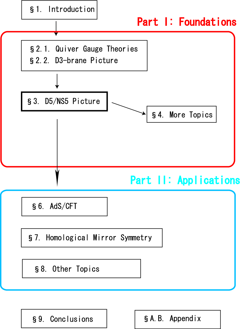
This review is mainly intended for people in the string theory community, but some parts of it should be of interest to researchers in other areas, such as statistical mechanics and mathematics. The interested reader should also consult a nice review by Kennaway[41], which gives a concise summary of the subject.

Throughout this review we have tried to emphasize connection with various topics. We have chosen to do so in the hope of conveying you the richness of the subject. We hope by going through this review, the reader can find many unexpected connection with various topics. At the same time, however, this makes this review slightly long with many references. Thus we have made some suggestions below to readers of certain backgrounds, although they should not be taken too seriously. In any case, We recommend §3, since that is the most important section in this paper.

•

Readers interested in physical interpretations or computational methods of brane tilings are strongly encouraged to read §3. If you have more time, you can pick up some materials in §4.
•

Readers interested in $AdS_{5}/CFT_{4}$ correspondence for Sasaki-Einstein manifolds should read §5. This section can be read almost independently. You should also consult some materials in §3 as needed.
•

Readers wanting to use brane tilings in string-phenomenological model building should read §3, discussion of fractional branes and flavor branes in §4.1 and §4.2, and relevant part of §7.1, in combination some materials from the paper [6].
•

Readers (including mathematicians) interested in homological mirror symmetry are encouraged to read §4.8 and §6, after skimming through §3, in combination with original works [1, 2, 3].

Although we have tried to cover many materials in this field, certainly we have not covered all the topics. We would like to apologize in advance for any important omissions.

Finally, this paper is based on the author’s Master’s thesis submitted in January 2008 to Department of Physics, Faculty of Science, the University of Tokyo, and was defended in February 2008. Most of this paper is based on previous literature in this field, and in particular the author’s papers and some works in progress [1, 2, 3, 4, 5, 6, 7]. However, we tried in this review to clarify points which are not explicitly stated, and some of the explanations we believe are new.

Part I Foundations of brane tilings

2 Quiver gauge theories from toric Calabi-Yau cone

In this section, we give a quick overview of $\mathcal{N}=1$ superconformal quiver gauge theories and their string theory realizations using D3-branes and Calabi-Yaus. Readers already familiar with earlier developments in quiver gauge theories can skip §2.1 and refer back to it as needed.

2.1 Preliminaries on quiver gauge theories

2.1.1 Quiver diagram and quiver gauge theories

The term ‘quiver’ was first introduced into mathematics by a mathematician Gabriel in the early 70’s[42] (actually, instead of ‘quiver’ he used the German word ‘Köcher’.). Although dictionary meaning of quiver is ‘‘a portable case for holding arrows’’, in physics and mathematics quiver (or quiver diagram) simply means an ‘‘oriented graph’’. By an oriented graph we mean a collection of vertices (nodes) and oriented edges (links, arrows)⁵⁵ 5 In this paper, we make no distinction between the words ‘vertex’ and ‘node’. The same applies to the words ‘edge’ and ‘link’.. Some examples of quiver diagrams are shown in Figure 7.

Note in some cases some arrows might start from one vertex and end at the same vertex. Also, in general we have multiple arrows going from one vertex to another⁶⁶ 6 It is said that oriented graphs we consider here are called ‘quivers’ because multiple arrows as in Figure 7 look similar to arrows in stored in a case., as shown in Figure 7.

When we have multiple arrows between two vertices, two different representations are used as in Figure 8, but they both represent the same quiver.

So far, a quiver is simply a graph, but then what is the real meaning of this graph in physics? To a physicist, choosing a quiver means to specify a gauge theory (quiver gauge theory). Let us explain how to construct a gauge theory from a quiver diagram.

•

First, to each vertex we associate a gauge group $U(N)$ . We do not bother about the differences between $U(N)$ and $SU(N)$ for the most of this paper . The rank $N$ of the gauge group can differ from one vertex to another, as we will discuss in §4.1, but for the moment we simply take all to them to be $N$ .

Also, although it is also possible to extend the construction to other gauge groups, e.g. $SO$ or $Sp$ , we restrict attention to $U(N)$ case for the moment. $SO$ and $Sp$ gauge groups appear in orientifolded brane tilings[43, 6]. See also §7.1 for brief discussion.
•

Second, to each oriented edge, we assign a bifundamental field. This field transforms as fundamental with respect to the gauge group at the startpoint of the edge, and anti-fundamental with respect to the gauge group at the endpoint (Figure 9). When we have multiple edges, we have precisely as many bifundamentals as the number of edges.

Figure 9: An arrow in a quiver diagram represents a bifundamental field, which transforms as $(\bar{N_{1}},N_{2})$ under $SU(N_{1})\times SU(N_{2})$ gauge groups.

For example, as a special case, when the startpoint and endpoint of an arrow coincide, the bifundamental field is an adjoint representation of the gauge group. In this sense, bifundamentals are generalization of adjoint representations⁷⁷ 7 In orbifold case, bifundamental fields actually come from adjoint scalars in $\mathcal{N}=4$ theories.. We can also consider inclusion of fundamentals and antifundamentals as will be explained in §4.2, and anti-symmetric and symmetric representations in orientifolded brane tilings 7.1.

So far, we have not specified spacetime dimension, but throughout this review, all quiver gauge theories are defined in four spacetime dimensions. Also, in this review we only consider theories with at least $\mathcal{N}=1$ supersymmetry (in some examples we have $\mathcal{N}=4$ or $\mathcal{N}=2$ supersymmetry). In other words, we are going to consider four-dimensional $\mathcal{N}=1$ supersymmetric quiver gauge theories.

In order to actually specify $\mathcal{N}=1$ theory, quiver diagram is not enough and we need to know superpotential (we simply assume that the Kähler potential is canonical). We thus need quiver diagram and superpotential to actually specify four-dimensional $\mathcal{N}=1$ supersymmetric quiver gauge theories. We are going to return to superpotentials later in §3.1.3, when we discuss the relation between fivebrane diagrams and quiver gauge theories.

2.1.2 Cancellation of gauge anomalies

The important thing to notice is that quiver gauge theories are in general chiral and we have non-trivial condition for cancellation of anomalies. In order to write down this condition, we label vertices of quiver diagram by $a,b,\ldots$ and edges by $I,J,\ldots$ . For an edge $I$ and one of its endpoint $a$ , define $\sigma(I,a)$ by

\sigma(I,a)=\begin{cases}+1&\textrm{ (when $a$ is an endpoint of $I$), }\\ -1&\textrm{ (when $a$ is a startpoint of $I$).}\end{cases}

(2.1)

Suppose we have gauge group $SU(N_{a})$ at each vertex $a$ . Then, using the definition as in (2.1), the gauge anomaly cancellation⁸⁸ 8 For $SU(2)$ case, we do not have ordinary gauge anomaly, but we should care about global anomaly (Witten’s anomaly) [44]. with respect to gauge group at vertex $a$ is represented by

\sum_{\genfrac{}{}{0.0pt}{}{I}{I=(a,b)}}\sigma(I,a)N_{b}=0,

(2.2)

where the summation is over all edges $I$ one of whose endpoints is $a$ , and the other endpoint is denoted $b$ . The rank of the gauge group at vertex $b$ is denoted $N_{b}$ . For the discussion in §4.1, let us rewrite (2.2) in another form. Define $\sigma(a,b)$ for two gauge groups $a,b$ (connected by an edge $I$ ) by

\sigma(a,b)=\sigma(I,a).

(2.3)

In other words, for two vertices $a,b$ of the quiver digram connected by an edge $I$ , $\sigma(a,b)=+1$ if the bifundamental field $I$ transforms as $(N_{a},\bar{N_{b}})$ under $SU(N_{a})\times SU(N_{b})$ , and $\sigma(a,b)=-1$ if $I$ transforms as $(\bar{N_{a}},N_{b})$ . Then (2.2) is rewritten as

\sum_{b\in a}\sigma(b,a)N_{b}=0,

(2.4)

where $b\in a$ means that $b$ is adjacent to $a$ . Also, in general there are several edges connecting $a$ and $b$ , and in that case the summation over all such edges is implicitly taken in the formula (2.4).

Let us explain the origin of this formula. An arrow which starts at edge $a$ and ends at edge $b$ corresponds to a bifundamental transforming as $(\overline{N_{a}},N_{b})$ under $SU(N_{a})\times SU(N_{b})$ . From the viewpoint of $SU(N_{a})$ gauge group, this bifundamental looks like a set of $N_{b}$ anti-fundamentals, which contributes $-N_{b}=\sigma(I,a)N_{b}$ to gauge anomaly. An arrow with opposite orientation then contributes with opposite sign and is again given by $\sigma(I,a)N_{b}$ . The condition for vanishing of the total gauge anomaly is therefore given by (2.2).

As an example, let us take the example of the quiver shown in Figure 10. In this example, (2.2) simply says

N_{1}=N_{3},\ \ N_{2}=N_{4}.

(2.5)

Thus we have $(N_{1},N_{2},N_{3},N_{4})=(N,N+M,N,N+M)$ , where $N$ is a non-negative integer and $M$ is an integer with $N+M\geq 0$ . Here appearance of $M$ means we can assign different ranks to difference vertices, and this corresponds to fractional branes in the Calabi-Yau setup explained in §2.2. The meaning of such anomaly-free rank assignments from fivebrane viewpoint will be discussed in §4.1.

Consider the special case where $N_{a}$ are the same for all vertices. Then the condition (2.2) simply means that, for each vertex $a$ , the number of incoming and outgoing arrows are the same. This condition is satisfied for the quiver in Figure 10. We will see in §3.1 that this condition is automatically satisfied for all quiver gauge theories realized by brane tilings.

2.2 Quiver gauge theories from D3-branes and Calabi-Yau

2.2.1 Orbifold singularities

Perhaps the reader might wonder at this point why we want to study such complicated quiver gauge theories. Certainly, we have many motivations, as we amply discuss in this review. Here we give one important motivation: quiver gauge theories appear quite naturally in string theory compactifications.

Historically speaking, this is actually the original motivation to study quiver gauge theories. In 1994 celebrated work, Douglas and Moore[45] has discovered that, by probing ALE spaces by D-branes, we have four-dimensional $\mathcal{N}=2$ superconformal quiver gauge theories on the probe D-branes. More specifically, let $\Gamma$ be a discrete subgroup of $SU(2)$ . Such discrete subgroup is classified completely by Felix Klein[46] (see Table 1). Interestingly enough, this classification coincides with the classification of semisimple simply-laced Lie algebras (Figure 11).

Table 1: Classification of discrete subgroups of

SU(2)

. More precisely, the subgroups shown below is that of

SO(3)

, and corresponding lift to

SU(2)

is called with ‘binary’ in front, such as “binary tetrahedral group”. This classification is in one-to-one correspondence with the classification of Dynkin diagrams, or semisimple Lie algebras, as shown in Figure 11.

$A_{n}$	cyclic
$D_{n}$	dihedral
$E_{6}$	tetrahedral
$E_{7}$	octahedral
$E_{8}$	icosahedral

Consider the orbifold space $\mathbb{C}^{2}/\Gamma$ , whose resolutions are called Asymptotically Locally Euclidean (ALE) spaces. Then the question is what kind of gauge theory we have on the stack of $N$ D-branes. Then answer[45, 47, 48] is that the theory is quiver gauge theory, with the quiver diagram given as follows.

Consider discrete subgroup $\Gamma$ of $SU(2)$ , and denote the set of all irreducible representations by $\{\rho_{i}\}$ . Since $\Gamma$ is a subgroup of $SU(2)$ (which acts on $\mathbb{C}^{2}$ ), we can consider standard two-dimensional representation denoted by $\rho_{r}$ . Then decompose the tensor product into irreducible representations:

\displaystyle\rho_{r}\bigotimes\rho_{i}=\bigoplus_{j}a^{ji}\rho_{j}.

(2.6)

From this decomposition we obtain a quiver diagram as follows. First, prepare a node for each irreducible representation $\rho_{i}$ . Next, write $a^{ij}$ arrows starting from the node $\rho_{i}$ and ending at $\rho_{j}$ . The supersymmetric quiver gauge theory specified by such quiver diagram is the theory we have on the D-branes probing $\mathbb{C}^{2}/\Gamma$ .

We have another way to write quiver diagram from $\Gamma$ . The quotient space $\mathbb{C}/\Gamma$ has a rational double point at the origin. Take a minimal resolution of this space, and we have exceptional divisors. Then we have a graph as a dual of the configuration of exceptional divisors.

Interestingly enough, the quiver diagram obtained from $\Gamma$ by these two different methods coincide, and moreover is exactly the same with the extended Dynkin diagram of ADE type, shown in Figure 11. This is famous McKay correspondence[49] (see [50, 51] for reviews) ⁹⁹ 9 In §3.1.3, we explain one more method to obtain quiver diagram from $\Gamma$ .. Thus McKay correspondence has a natural role to play in string theory!

Moreover, if we consider the moduli space of these $\mathcal{N}=2$ quiver gauge theories, the moduli space coincides with the ALE space itself, which is the elegant physical realization of the hyperKähler construction of ALE spaces[52] in mathematics.

We can generalize this discussion to subgroup $\Gamma$ of $SU(3)$ . The classification of such $\Gamma$ was done by Blichfeldt in 1917[53], although in this case classification is much more subtle. Similar to $SU(2)$ case, we consider the orbifold $\mathbb{C}^{3}/\Gamma$ . Such orbifolds leave $\mathcal{N}=1$ supersymmetry, and the corresponding gauge theory is the $\mathcal{N}=1$ supersymmetric quiver gauge theory.

Again from the rules (2.6), we can write down the corresponding quiver diagram by decomposition of representation, which is a trivial generalization¹⁰¹⁰ 10 The only complication in $SU(3)$ case is that we also need superpotential, since SUSY is broken down to $\mathcal{N}=1$ . For Abelian orbifolds, superpotential is obtained by brane tiling techniques, as we will explain in later sections. of the $SU(2)$ case. For examples of non-Abelian orbifolds, see [54, 55]. Here we only consider Abelian orbifolds. As a simple example, we show in Figure12 the McKay quiver corresponding to $\mathbb{Z}_{5}$ orbifold of $\mathbb{C}^{3}$ , with the $\mathbb{Z}_{5}$ action given by $(z_{1},z_{2},z_{3})\to(\omega z_{1},\omega^{2}z_{2},\omega^{2}z_{3})$ (here $\omega^{5}=1$ ). Such a discrete subgroup is sometimes denoted $(1,2,2)/5$ .

More generally, if we consider the orbifold $(1,p,q)/(1+p+q)=\mathbb{Z}_{1+p+q}$ , we have the quiver shown in Figure 13. These McKay quivers will appear again in §3.1.3, in the discussion of brane tilings.

2.2.2 Toric Calabi-Yau singularities

The orbifold examples we have been discussing so far are interesting, but we want to consider more general case. Of course, if we consider arbitrary Calabi-Yau, we are completely at a loss, since for non-orbifold case we no longer have the rules as in (2.6). Our strategy here is to concentrate on toric Calabi-Yau three-folds (although we will refer to non-toric case as well in some parts of this review).

For reviews of toric geometry, see excellent books[56, 57], and the physics paper[58]. Here we remind the reader that toric Calabi-Yau manifold is a special class of Calabi-Yau manifold which is specified by a convex polytope, the so-called toric diagram (or more precisely, fan). In other words, everything we need to know about toric Calabi-Yau are contained in the toric diagram, at least in principle. Of course, these are special class of Calabi-Yaus. For example. when $\Gamma\subset SU(2)$ is a DE-type discrete subgroup, $\mathbb{C}^{2}/\Gamma\times\mathbb{C}$ is not toric. It should be stressed, however, that toric Calabi-Yaus contains infinitely many examples of Calabi-Yaus and they constitute an important subclass of Calabi-Yau manifolds.

We now prepare non-compact Calabi-Yau 3-fold which have cone-type singularity. Then we probe this geometry by D3-branes (Figure 14), neglecting the possible back-reaction onto geometry. As shown in the Figure, D3-branes are placed transverse to Calabi-Yau.

Also, by a cone we mean a Calabi-Yau 3-fold, which is obtained from some five-dimensional manifold $(S,g_{S})$ by the metric cone construction¹¹¹¹ 11 Such manifolds, i.e., manifolds whose metric cone is Calabi-Yau, are called Sasaki-Einstein manifolds and going to play an important role in AdS/CFT, as we will see in section §5.. That is, the metric of Calabi-Yau $(C(S),g_{C(S)})$ can be expressed in the form

ds_{C(S)}^{2}=dr^{2}+r^{2}ds^{2}.

(2.7)

The manifold $(S,g_{S})$ is called toric Sasaki-Einstein manifolds, which is the topic of §5.

Since the Calabi-Yau is non-compact, and the volume of Calabi-Yau is infinite, gravity decouples and we have gauge theory on these probe D-branes. The moduli space of this gauge theory should coincide with the toric Calabi-Yau cone. The general belief since 90’s was that the gauge theory is a quiver gauge theory, at least for toric Calabi-Yaus. But in this general setting, it is not obvious at all which Calabi-Yau gives which quiver gauge theory. Since toric Calabi-Yaus are specified by the toric diagram and since quiver gauge theories are specified by the quiver diagram, the problem is how to translate the geometry (toric diagram) into gauge theory (quiver diagram) (Figure 15).

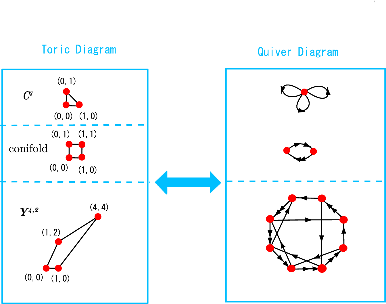
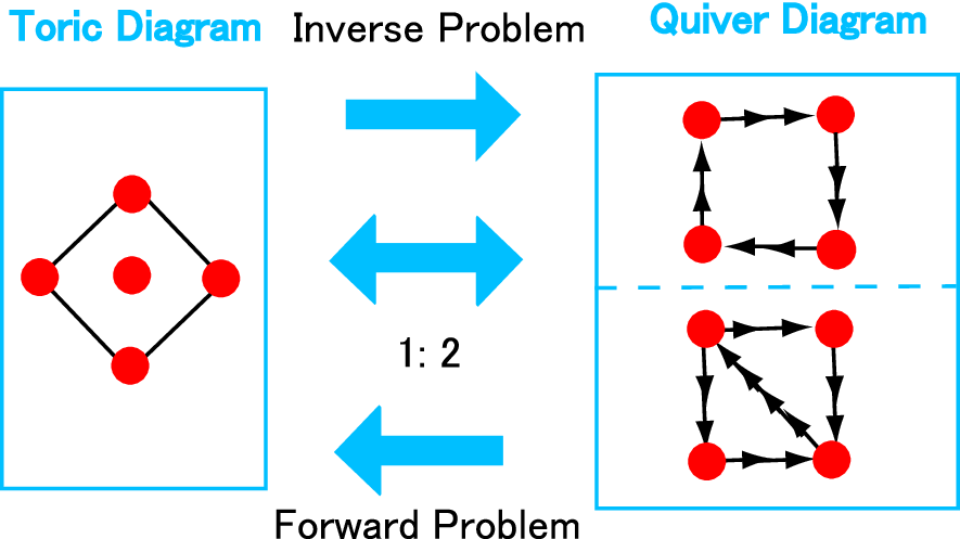
In the literature, the problem of obtaining toric diagram from quiver diagram is called the forward problem, and other direction, namely the problem of obtaining quiver diagram from toric diagram, is called the inverse problem. The reason for these names is that in general several different quivers correspond to the same toric diagram, and the correspondence between toric diagrams and quiver diagrams are in general one-to-many (see Figure 16). This phenomena is dubbed “toric duality”, and it is believed[59] that this is related to the Seiberg duality[60]. We will discuss this point more in detail in §4.7.

If you look at this correspondence from a slightly different viewpoint, you will see that it is essentially the setup of AdS/CFT correspondence. If you consider the back-reaction of D-branes onto geometry, we have AdS near-horizon geometry¹²¹² 12 However, when we consider other ingredients, such as fractional branes, the gauge theory is not necessarily conformal. See §4.1 for discussion on fractional branes.. AdS/CFT in this case states that type IIB string theory on $AdS_{5}\times S$ is equivalent to four-dimensional $\mathcal{N}=1$ superconformal quiver gauge theories. This will be studied in detail in §5.

So, the problem is to find the precise relation between toric diagrams and quiver diagrams. Before the discovery of brane tilings, we have no efficient way to answer this question. Although general algorithm already existed[61] using partial resolutions, computation often becomes unpractical as the toric diagram becomes more and more complicated. Also, that method does not tell you about the superpotential of $\mathcal{N}=1$ theories.

All these problems are solved by the method of brane tilings, as we will see. Brane tiling gives us “fast forward algorithm” and “fast inverse algorithms” which solve these problems. But before describing the details of such algorithms, we should explain the physical meaning of brane tilings.

2.3 Summary

In this section, we prepared some basic knowledge needed to understand the rest of this paper. In §2.1, we briefly reviewed quiver diagram and quiver gauge theories. The condition for gauge anomaly cancellation was also discussed. In §2.2, we described stringy realization of quiver gauge theories from non-compact Calabi-Yaus probed by D3-branes. For the orbifold case, the story is well-known, but for more general toric Calabi-Yaus, we do not know the precise relation between toric diagram and quiver diagram. As we will see in the next section, fivebrane configurations represented by brane tilings give a clear-cut answer to this problem.

3 Brane tiling as a fivebrane system

In this section we explain configuration of D5-branes and NS5-brane which is represented by a bipartite graph. This fivebrane system provides string theory realization of a four-dimensional $\mathcal{N}=1$ superconformal quiver gauge theory. Along the way we will see a clear physical interpretation of brane tilings. The explanation of this section is an expanded version of part of §1 of our paper[5].

3.1 The strong coupling limit

3.1.1 Step-by-step construction of fivebrane systems

The goal of this subsection is to construct a fivebrane system which represents a $\mathcal{N}=1$ superconformal quiver gauge theory. The final fivebrane system is slightly complicated, so we proceed step by step.

As a first step, we consider type IIB string theory and a stack of $N$ D5-branes. Then, as is well-known, we have $U(N)$ (or $SU(N)$ ) gauge theory on the D5-branes. Here we do not bother the difference of $U(N)$ and $SU(N)$ because $U(1)$ factor decouples in IR ¹³¹³ 13 However, these $U(1)$ s play crucial roles in the discussion of baryonic $U(1)$ global symmetries in §5.5..

Since we want to have four-dimensional gauge theories, two of six directions of D5-branes are redundant. We therefore choose to compactify two spatial directions on two-dimensional torus ${\mathbb{T}}^{2}$ with radius $R$ . Out of ten-dimensional spacetime coordinates $x^{0},x^{1},\ldots x^{9}$ ( $x^{0}$ being time coordinate and others spatial coordinate) we take $x^{5}$ and $x^{7}$ to be directions of ${\mathbb{T}}^{2}$ .

We now have $N$ D5-branes wrapping $\mathbb{T}^{2}$ . If $R$ is small and Kaluza-Klein modes decouple, we have four-dimensional $\mathcal{N}=4$ supersymmetric Yang-Mills theory. But this is certainly not what we want! We want gauge theory with multiple gauge groups, and we want to reduce supersymmetry down to $\mathcal{N}=1$ .

For those purposes we use another ingredient, NS5-brane. In order to obtain multiple gauge groups, we divide the D5 worldvolume using semi-infinite cylinder of NS5-branes, as shown in Figure 17, 18 and Table 2.

Although originally the same D5-brane, each D5-brane region is now separated by semi-infinite cylinder of NS5-branes, and each region has its own gauge group $SU(N)$ , and we have multiple gauge groups, as desired. Also, since the introduction of NS5-brane in two different directions leaves quarter of original $\mathcal{N}=4$ supersymmetry, we are left with $\mathcal{N}=1$ supersymmetry. Thus we have succeeded in obtaining both $\mathcal{N}=1$ SUSY and multiple gauge groups.

Table 2: Brane configuration corresponding to Figure 17 and 18. This is the conifold case, as will be explained below. The two directions (57) are compactified on

{\mathbb{T}}^{2}

. Compare with Figure 17 and Figure 18. We have two semi-infinite NS5-cylinders extending in 45-directions. We also have two in 67-directions, which are denoted by NS5’. Due to the introduction of NS5-brane in two directions, supersymmetry is broken to

\mathcal{N}=1

. In general, the brane configuration takes more general form shown in Table 3.

	0	1	2	3	4	5	6	7
D5	$\circ$	$\circ$	$\circ$	$\circ$		$\circ$		$\circ$
NS5	$\circ$	$\circ$	$\circ$	$\circ$	$\circ$	$\circ$
NS5’	$\circ$	$\circ$	$\circ$	$\circ$			$\circ$	$\circ$

But this is not the end of the story. In our brane configuration, we have junctions of D5-branes and NS5-brane. As first pointed out in [39], in order for the conservation of NS5-charge, the junction should be either (b) or (c) of Figure 19, depending on the orientation of NS5.

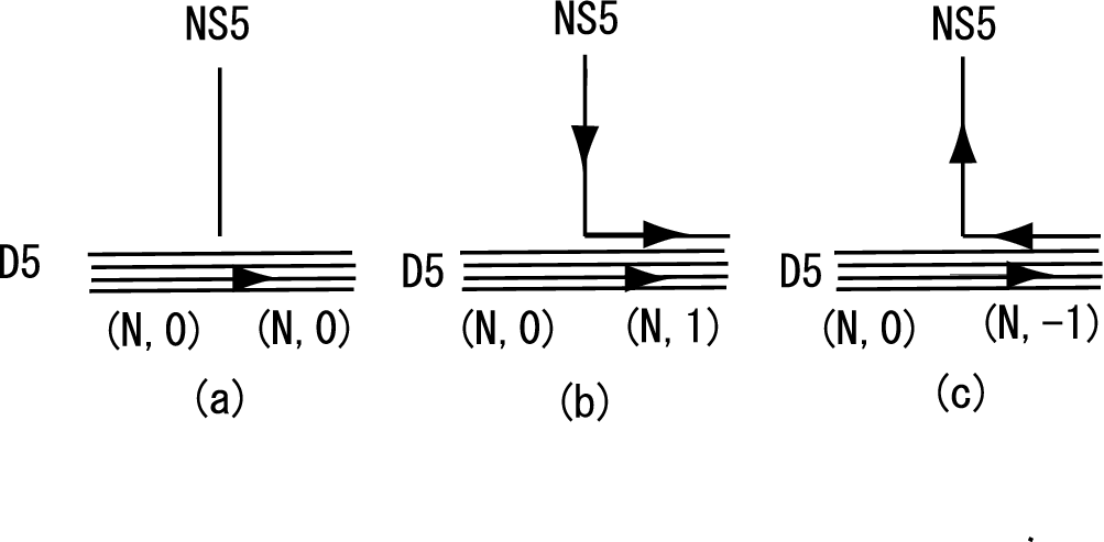
From this fact, we see that some regions of ${\mathbb{T}}^{2}$ becomes bound states of $N$ D5-branes and $1$ NS5-brane. In general, bound states of $N$ D5-branes and $k$ NS5-branes are called $(N,k)$ -branes. In the case $k<0$ , $(N,k)$ -brane is a bound state of $N$ D5 and $|k|$ NS5, with D5 and NS5 having opposite orientations. In this language, we should expect at least $(N,1)$ -branes and $(N,-1)$ -branes to appear. The example of such a division of $\mathbb{T}^{2}$ is shown in Figure 20. We call such diagrams fivebrane diagrams [6], since they represent the structure of fivebrane systems. In the fivebrane diagram, we have used the convention of NS5-charge as shown in Figure 21.

Interestingly enough, in general $(N,k)$ branes with $|k|\geq 2$ appear as in Figure 22. In this review, we do not discuss these cases for the most part, since we are not quite sure what kind theory we have on these branes¹⁴¹⁴ 14 Presumably that theory should be some deformation of ordinary quiver gauge theories, since by changing the position of cycles of NS5-branes we have a transition between the two theories.; at least, they are not conventional quiver gauge theories. (see, however, §4.3.2, particularly Figure 62 for discussion of such brane configurations.).

Now we know some consistency conditions are imposed on the NS5-cycles. Since 57-directions are torus, the NS5-charge should be the same after we go around an arbitrary cycle of ${\mathbb{T}}^{2}$ . More formally, let $\mbox{\boldmath$\alpha$}_{\mu}$ be the cycle of NS5-brane. Here $\mu$ runs from $1$ to $d$ , where $d$ is the number of cycles of NS5-brane. Let us denote the winding number of cycle $\mbox{\boldmath$\alpha$}_{\mu}$ by $(p_{\mu},q_{\mu})$ . Here $p_{\mu}$ and $q_{\mu}$ refers to the winding number in $\alpha$ and $\beta$ -cycles, respectively. Then we have

\sum_{\mu}p_{\mu}=\sum_{\mu}q_{\mu}=0,

(3.1)

\sum_{\mu=1}^{d}\mbox{\boldmath$\alpha$}_{\mu}=0\mbox{ in }H_{1}(\mathbb{T}^{2},\mathbb{Z}).

(3.2)

As an example, the configuration as in Figure 23 (a) is not allowed, but (b) is a consistent configuration.

Now we should look at NS5-branes slightly differently from previous discussions. In our previous discussions, we have simply put several NS5-branes orthogonal to D5. But now, we also have NS5-branes parallel to D5-branes, as shown in Figure 19. These seemingly different NS5-branes join together and we have a single NS5-brane! (see Figure 24 for example) As in (b) and (c) of Figure 19, one should also remember that the orientation of the NS5-brane is opposite in some regions.

Of course, it should be kept in mind that that the shape of NS5-brane is in some sense singular. For example, as can be seen from Figure 19, NS5-brane bends 90 degrees and change its direction suddenly at junctions. As we will explain later in 3.2, this is simply because we are considering some limit (the strong coupling limit) in which the brane configuration simplifies dramatically. The shape of NS5-brane is smooth for general string coupling constant, and in the weak coupling limit even becomes a holomorphic curve (see §3.3).

Since now we have single NS5-brane, the final brane configuration is, if you write NS5-worldvolume schematically as ${\mathbb{R}}^{3,1}\times\Sigma$ , the one shown in Table 3.

Table 3: The brane configuration corresponding to brane tilings. The directions 5 and 7 are compactified, and

\Sigma

is a two-dimensional surface in 4567 space. Note that all the semi-infinite cylinders of NS5-branes as in Table 2 now merge into a single NS5-brane. We have so far used the example of the conifold, but the surface

\Sigma

takes more general form, as we will explain.

	0	1	2	3	4	5	6	7	8	9
NS5	$\circ$	$\circ$	$\circ$	$\circ$	$\Sigma$
D5	$\circ$	$\circ$	$\circ$	$\circ$		$\circ$		$\circ$

We should still remember that $\Sigma$ is not an arbitrary two-dimensional surface in 4567-space. It intersects ${\mathbb{T}}^{2}$ with 1-cycle. That is, one of its two directions is in the compact 5,7-directions, and the other one is in non-compact 4,6-directions.

3.1.2 Relation with D3-brane picture

The Tables 2 and 3 are the key to understanding the relation with D3-brane setup discussed in §2.2. Since 5,7-directions are simply ${\mathbb{T}}^{2}$ , we can take T-duality along these directions. Then D5-branes are turned into D3-branes, and NS5-branes are now turned into geometry, actually a Calabi-Yau manifold (As we mentioned above, one of 5,7-directions are orthogonal to NS5, so we are taking T-duality perpendicular to NS5, which turns NS5 into geometry). The net result is shown in Figure 4. You will immediately notice that this is precisely the setup of the D3-brane probing Calabi-Yau which we already discussed in §2.2.

Table 4: The brane configuration obtained by taking T-duality in 5,7-directions of the fivebrane systems shown in Table 3. D5-branes are turned into D3-branes, and NS5-brane is turned into a toric Calabi-Yau manifold. The system obtained by this way is precisely Calabi-Yau setup with D3-branes, which we already discussed in §2.2.

	0	1	2	3	4	5	6	7	8	9
CY3					$\circ$	$\circ$	$\circ$	$\circ$	$\circ$	$\circ$
D3	$\circ$	$\circ$	$\circ$	$\circ$

At this point you can understand why we started from D5-branes, with two spatial directions compactified. From D3-brane picture, the torus ${\mathbb{T}}^{2}$ are subtorus of the $U(1)^{3}$ -isometry of toric Calabi-Yau, and we have taken T-duality along that ${\mathbb{T}}^{2}$ to turn Calabi-Yau into NS5-brane.

The important point here is that by taking T-duality, Calabi-Yau geometry is turned into NS5-branes. Although NS5-brane contains essentially the same information as Calabi-Yau, by taking appropriate limit NS5-branes become flat and we are left with brane configurations in flat spacetimes! This is the beauty of Hanany-Witten[62] type construction (see [63] for extensive review).

We should perhaps stress here that this is not the only way to use NS5-brane. For example, even before the discovery of brane tiling, we have many literature on realizing chiral gauge theories using type IIA theory with NS5-brane and D4-branes [64, 65, 66]. The type IIA picture, although simple, is limited to orbifolds and generalized conifolds (and their orientifolds) and as we will see, D5/NS5-configurations we consider here are by far the most powerful and applies to arbitrary toric Calabi-Yau 3-fold.

A short reminder of toric geometry

We still haven’t discuss how to specify NS5-cycles $\mbox{\boldmath$\alpha$}_{\mu}$ on torus. This choice should reflect the choice of the toric diagram. In order to see the connection, let us spend some time recalling some basic facts in toric geometry.

Let us start from a toric Calabi-Yau cone $\cal M$ described by a toric diagram. In this paper we only consider three-dimensional Calabi-Yau manifolds. Let $v_{i}\in\Gamma=\mathbb{Z}^{3}$ be the set of lattice points in the toric diagram. By $SL(3,\mathbb{Z})$ transformation, we can take the coordinate system in which the components of $v_{i}$ are given by

v_{i}=(p_{i},q_{i},1).

(3.3)

The toric diagram is ordinary represented as a two-dimensional diagram by using the first two components of these vectors. An example of $\mathbb{C}^{3}$ case is shown in Figure 25 (a).

We define¹⁵¹⁵ 15 The reader should be careful when comparing with literature, because $\mathcal{C}^{*}$ is sometimes also written as $\mathcal{C}$ . Our notation is in accord with the fact that $\mathcal{C}^{*}$ is in the dual of Lie algebra of torus. the dual cone ${{\cal C}^{*}}$ as the set of vectors $w\in\mathbb{R}^{3}$ satisfying

v_{i}\cdot w\geq 0\quad\forall i.

(3.4)

When we consider resolutions of the toric Calabi-Yau, Kähler parameters come to the right hand side of this inequality. In this paper we will not discuss such resolutions and the right hand side is always zero. In such a case we do not have to use all $v_{i}$ to define ${{\cal C}^{*}}$ by (3.4), and we only need $v_{\alpha}$ corresponding to the corners of the toric diagram. Here symbols $\alpha,\beta\ldots$ is used to denote lattice points in the corners of toric diagram, and $i,j\ldots$ denotes all the lattice points in the toric diagram (including its boundary). We further assume that the label $\alpha$ increase one by one as we go around the perimeter of toric diagram in counterclockwise manner. The boundary of the dual cone $\partial{{\cal C}^{*}}$ consists of flat faces called facets. Each facet corresponds to each vector $v_{\alpha}$ ,and is defined as the set of points satisfying $v_{\alpha}\cdot w=0$ and $v_{\beta}\cdot w\geq 0~~(\forall\beta\neq\alpha)$ . We denote the facet corresponding to $v_{\alpha}$ by $F_{\alpha}$ . The structure of the base manifold ${{\cal C}^{*}}$ is conveniently expressed as a planar diagram by projecting the facets onto a two-dimensional plane by simply neglecting the third coordinate. It is called a web-diagram. Figure 25 (b) is an example of web-diagram for $\mathbb{C}^{3}$ . The lines in the web-diagram represent the edges of the base manifold ${{\cal C}^{*}}$ .

We can regard the Calabi-Yau manifold as the $\mathbb{T}^{3}$ -fibration over the dual cone ${{\cal C}^{*}}$ (3.4), although strictly speaking some cycles of $\mathbb{T}^{3}$ shrinks on facets as we will explain. Let $(\phi_{1},\phi_{2},\phi_{3})$ be the coordinates in the toric fiber. We choose the period of each coordinate to be $2\pi$ . We can regard $\Gamma$ as the lattice associated with the toric fiber $\mathbb{T}^{3}$ . Namely, we can associate points in $\Gamma$ with cycles in $\mathbb{T}^{3}$ . By this identification, we can regard an arbitrary non-vanishing vector $v\in\Gamma$ as a generator of $U(1)$ isometry of the $\mathbb{T}^{3}$ .

On a facet $F_{\alpha}$ the cycle specified by $v_{\alpha}$ in $\mathbb{T}^{3}$ fiber shrinks and the fiber becomes $\mathbb{T}^{2}$ . In order to parameterize the $\mathbb{T}^{2}$ fiber on each facet, the following coordinate change is convenient¹⁶¹⁶ 16 Strictly speaking, we should write ${\theta_{i}}^{\alpha}$ since $\theta_{i}$ depends on facet $\alpha$ . In this review, we do not show the $\alpha$ -dependence explicitly for notational convenience..

(\phi_{1},\phi_{2},\phi_{3})=\theta_{1}(1,0,0)+\theta_{2}(0,1,0)+\theta_{3}(p_{i},q_{i},1).

(3.5)

This is equivalent to

\theta_{1}=\phi_{1}-p_{\alpha}\phi_{3},\quad\theta_{2}=\phi_{2}-q_{\alpha}\phi_{3},\quad\theta_{3}=\phi_{3}.

(3.6)

On the facet, the $\theta_{3}$ -cycle shrinks and $(\theta_{1},\theta_{2})$ is a pair of good coordinates on $\mathbb{T}^{2}$ .

T-duality and Buscher’s rule

After a brief review of toric geometry, we now want to apply T-duality along the two-cycle. Basically, T-duality is taken along $\phi_{1},\phi_{2}$ -directions. As we have seen, however, these are in general not good coordinates since we have shrinking cycles. Instead, we choose to use coordinates $\theta_{1},\theta_{2}$ for each facet $\alpha$ ¹⁷¹⁷ 17 Thus we are taking T-duality in each patch of the manifold. This is somehow similar to the recent work of [67]..

Recall that T-duality exchanges momentum and winding. This means corresponding gauge fields, i.e. metric and B-field, should also be exchanged. In the original Calabi-Yau picture, we have no NS-NS B-field, but the metric is not flat. After T-duality, we have a non-trivial B-field, which is the source of NS5-brane. This is represented in general by Buscher’s rule explained in Appendix §A. After applying the Buscher’s rule (A.13) twice, we have non-trivial B-field

B=v_{1}\wedge(d\theta^{1}+v_{1})+v_{2}\wedge(d\theta^{2}+v_{1}),

(3.7)

where $v_{1}$ and $v_{2}$ are gauge fields in $\theta_{1}$ and $\theta_{2}$ -directions, respectively. The important thing is that this B-field is dependent on the choice of the facet $\alpha$ . Since $\theta$ is related to $\phi$ as in (3.6), the value of $B$ jumps as we go from one facet $\alpha$ to another $\alpha+1$ :

B\to B-(\Delta p\ v_{1}+\Delta q\ v_{2})\wedge d\theta_{3},

(3.8)

where $\Delta p=p_{\alpha+1}-p_{\alpha},\Delta q=q_{\alpha+1}-q_{\alpha}$ . This signifies the presence of NS5-brane in the intersection of $F_{\alpha+1}$ with $F_{\alpha}$ (See Figure 26). ¹⁸¹⁸ 18 In principle, we can compute the jump of NS-charge by integrating the difference (3.8) over $S^{3}$ . This is difficult in practice, since we do not know the explicit form of the metric. Consequently, semi-infinite cylinder of NS5-branes should be extending in the direction of the primitive normals to the toric diagram, as in Figure 18. To put in other terms, the web diagram coincides with junction of semi-infinite cylinders of NS5-branes.

This is familiar in the simple example shown in Figure 27. In this case, $\mathbb{C}\times\mathbb{C}^{2}/\mathbb{Z}_{2}$ is turned into two parallel NS5-branes. More generally, it is well-known that T-duality maps $A_{n}$ singularity to $n$ parallel NS5-branes, and you can directly verify this fact using explicit metric.

Our discussion for general toric Calabi-Yau is a generalization of this well-known fact, although it is often difficult to verify this fact directly using explicit form of the metric. You might think this is a pity, but at the same time it is good, since it is often extremely difficult to find explicit metrics and we do not need to know them for most of our purposes.

We have understood our brane configuration in 46-directions, but what about 57-directions? Since we are using smeared solution in SUGRA (see Appendix A), Buscher rule does not tell us anything about $\mathbb{T}^{2}$ -directions we want to know. But BPS conditions dictates $\Sigma$ is Lagrangian, namely the Kähler form in 4567-space

\omega=dx_{4}\wedge dx_{5}+dx_{6}\wedge dx_{7}

(3.9)

should vanish on NS5-brane. This means that when a NS5-brane span $(p,q)$ -directions in 46-directions, it should be extending in $(q,-p)$ -direction in 57-directions. The net result is that we have 1-cycle of NS5-brane on $\mathbb{T}^{2}$ with winding $(q,-p)$ for each primitive normal $(p,q)$ of the toric diagram. By rotating 90 degrees for convenience, NS5-cycle is turned into 1-cycle with winding $(p,q)$ , namely the same winding number with the primitive normal of the toric diagram. We are going to use this convention throughout the rest of the paper.

Summarizing, shrinking cycles of winding number $(p,q)$ are mapped by T-duality (and 90 degrees rotation in 57-space) to NS5-brane wrapping cycles of winding number $(p,q)$ . This means in particular that previously defined $d$ , which is the number of cycles of NS5-branes, is equal to number of lattice points on the boundary of the toric diagram. Note also that the consistency conditions discussed previously in (3.1) is trivially satisfied (it amounts to the condition that if we go around the perimeter of toric diagram, then we are back to the same place). By this way we now understand the relation with toric Calabi-Yau and NS5-cycles.

Examples are shown for $\mathbb{C}^{2}/\mathbb{Z}_{2}\times\mathbb{C}$ (Figure 28) and $\mathbb{C}^{3}/\mathbb{Z}_{5}$ with $\mathbb{Z}_{5}=(1,2,2)/5$ (Figure 29). These orbifold examples are discussed previously in Calabi-Yau setups in §2.2.

3.1.3 Relation with quiver gauge theories

Up to now we have discussed fivebrane systems and their relation with toric Calabi-Yau manifolds. We now discuss the precise relation between fivebrane systems and quiver gauge theories.

From fivebrane systems to quiver gauge theories

The question we want to ask is what kind of gauge theories we have on fivebrane systems.

As already said, each $(N,0)$ -brane region corresponds to a $SU(N)$ gauge group. How about $(N,1)$ -branes and $(N,-1)$ -branes? Do we have $SU(N)$ gauge groups also on these branes in the low-energy effective field theory? In fact, the answer is no. We have only $U(1)$ on $(N,\pm 1)$ -branes, as can be seen by applying $SL(2,\mathbb{Z})$ -transformation. This shows that only regions of $(N,0)$ -brane corresponds to vertices of the quiver diagram.

Some readers might worry about the $U(1)$ gauge group that we have not taken account of. For example, $(N,\pm 1)$ -branes couple to $(N,\pm 1)$ -branes ¹⁹¹⁹ 19 In general, only $(p,q)$ -strings can end on $(p,q)$ -branes. You can see this fact by applying $SL(2,\mathbb{Z})$ -duality to D-brane, which couples to the fundamental string. and we have seemingly a $U(1)$ gauge field. However, as analyzed in [39], that $U(1)$ gauge field is fixed by the boundary conditions at junctions and therefore not dynamical. That $U(1)$ is only a global symmetry, and is identified with one of the global anomalies of $\mathcal{N}=1$ superconformal quiver gauge theories [40].

Next, for each intersection point of $(N,0)$ -branes, we have massless open strings, which corresponds to bifundamental fields in quiver gauge theories. Due to the presence of NS5-brane, only strings in one direction is allowed and the theory becomes chiral (Figure 30).

You can understand this fact as follows. We explain in the conifold example for simplicity. In the conifold example shown in Table 2, we have two types of NS5-branes, NS5 and NS5’. If we remove NS5’, we have four-dimensional $\mathcal{N}=2$ superconformal quiver gauge theory. In particular, we have $\mathcal{N}=2$ matter hypermultiplets. The scalar degrees of freedom of this multiplet is four (when counted as real) and this corresponds to the move of D5-brane in 6789 space. Now put NS5’ back, and supersymmetry is broken down to $\mathcal{N}=1$ . In this process, $\mathcal{N}=2$ hypermultiplet is broken down into two $\mathcal{N}=1$ chiral multiplets. However, due to the presence of NS5’, D5-brane can no longer move freely in 67 directions and this means that only one of two chiral multiplets remains. This explains that we have a chiral gauge theory. This feature, that the gauge theory is chiral, is extremely important because our world is described by chiral gauge theories but it is often not easy to realize chiral gauge theories from string theory.

Now, from above considerations it is clear that we have quiver gauge theories on D5-branes. Each $(N,0)$ -region corresponds to a vertex of the quiver diagram, and we need an arrow of the quiver diagram for each intersection point of $(N,0)$ -brane. An example of the quiver diagram read off from fivebrane diagram is shown in Figure 31. More examples, corresponding to $\mathbb{C}^{3}$ and the conifold, are also shown in Figure 32 and Figure 33. You can also verify that bipartite graphs in Figure 5 give quiver diagrams as in Figure 7.

We also show in Figure 34 and 35 the quiver diagrams corresponding to fivebrane diagrams in Figure 28 and 29,

Note that these are exactly the same as the quivers shown in Figure 11 and 12, respectively. More generally, we can prove

Theorem 3.1.

Let $\Gamma$ be an Abelian discrete subgroup of $SU(3)$ , and let $\Delta$ be a toric diagram whose corresponding Calabi-Yau is the orbifold $\mathbb{C}^{3}/\Gamma$ . Then the quiver (and superpotential)²⁰²⁰ 20 Mathematically speaking, superpotential (or its F-term relations) is an ideal in the path algebra of quiver. See §6.2.3. obtained from the method discussed here coincides with the McKay quiver of $\Gamma$ .

Recall that McKay quiver is obtained from $\Gamma$ by decomposing tensor product of representations (see (2.6)). The proof of this statement is combinatorial in nature and can be found in [1]. In §2.2.1, we have explained two different methods to obtain quiver diagram from $\Gamma$ . We now have another, and these three methods all give the same answer.

We have now verified our original claim that fivebrane systems realize four-dimensional $\mathcal{N}=1$ supersymmetric quiver gauge theories, but fivebrane systems knows more than that. For example, we can read off superpotentials. For each region of $(N,\pm 1)$ -brane, we can span a disk and thus we have tree-level disk amplitude of string theory interactions, which in turn means that we have such a term in superpotential, as in Figure 36.

More formally, for each face of $(N,\pm 1)$ -brane (which are labeled by $k$ ), we have superpotential terms like

h_{k}\mathop{\rm tr}\nolimits\prod_{I\in k}\Phi_{I},

(3.10)

where $I\in k$ means that bifundamental $I$ is around the face $k$ , and the product inside the trace is taken in clockwise (or counterclockwise, depending on the sign of NS5-charge) manner. Also, $h_{k}$ is a superpotential coupling (Yukawa coupling), and meaning of this parameter will be explored in full detail in §4.4.

The expression of superpotential is now given by

\sum_{k}h_{k}\mathop{\rm tr}\nolimits\prod_{I\in k}\Phi_{I}.

(3.11)

Here we simply take them to be

h_{k}=\begin{cases}+1&(k:(N,1)-\textrm{brane})\\ -1&(k:(N,-1)-\textrm{brane})\end{cases}.

(3.12)

The meaning of this choice will become clear in §4.4. Here we simply comment that it is chosen so that the theory becomes conformal and the corresponding geometry being toric Calabi-Yau cone.

Let me give you several examples of superpotentials. In $\mathbb{C}^{3}$ example of Figure 32, we have

W=\mathop{\rm tr}\nolimits(XYZ-XZY)=\mathop{\rm tr}\nolimits(X[Y,Z]),

(3.13)

which is the well-known superpotential of $\mathcal{N}=4$ super Yang-Mills. We can instead consider the superpotential

W=\mathop{\rm tr}\nolimits(e^{\sqrt{-1}\gamma}XYZ-e^{-\sqrt{-1}\gamma}XZY).

(3.14)

This deformation is the so-called $\beta$ -deformation of $\mathcal{N}=4$ gauge theory. It preserves $\mathcal{N}=1$ supersymmetry, but the corresponding geometry is no longer toric Calabi-Yau.

For Figure 33, we have

W=\mathop{\rm tr}\nolimits(A_{1}B_{1}A_{2}B_{2})-\mathop{\rm tr}\nolimits(A_{1}B_{2}A_{2}B_{1}).

(3.15)

This is again the famous superpotential corresponding to the conifold[68].

As a more complicated example, consider the case of SPP shown in Figure 31. In Figure 37 we have enlarged the fundamental region, so that superpotential is easily read off. The result is given by

W=\mathop{\rm tr}\nolimits(X_{21}X_{12}X_{23}X_{32}-X_{23}X_{33}X_{32}+X_{33}X_{31}X_{13}-X_{31}X_{12}X_{21}X_{13}).

(3.16)

If you look at several examples of superpotential, then you will notice that each bifundamental field $X_{I}$ is contained exactly twice in the superpotential, one in the term with plus sign and one minus sign. The superpotentials are therefore of the special kind. From fivebrane viewpoint, this follows because each bifundamental is located at the intersection of two $(N,0)$ -branes and one $(N,1)$ and one $(N,-1)$ -brane (see Figure 30).

In the language of Calabi-Yau geometry, this corresponds to the condition that the Calabi-Yau is toric (we sometimes say that superpotential $W$ satisfies toric condition). Suppose the superpotential takes the form

W=+\mathop{\rm tr}\nolimits(X_{I}X_{J}\ldots)-\mathop{\rm tr}\nolimits(X_{I}X_{K}\ldots)+(\textrm{terms independent of }X_{I}),

(3.17)

then the F-term equation $\frac{\partial W}{\partial X_{I}}=0$ takes the form

X_{J}\ldots=X_{K}\ldots,

(3.18)

i.e. (monomial)=(monomial). Since the vacuum moduli of quiver gauge theory corresponds to Calabi-Yau, this relation becomes part of defining equations of Calabi-Yau. Since toric geometry allow only relations of (monomial)=(monomial) form, this ensures that the Calabi-Yau is toric. This means that as long as we use brane tilings, we can only describe toric Calabi-Yaus, or their deformations (such as $\beta$ -deformation).

The connection with bipartite graphs

Perhaps the reader might be wondering at this point what has become of the bipartite graph we first encountered in Introduction (see Figure 5). So far, we have not mentioned bipartite graphs up to this point. In fact, in many cases we can simply use fivebrane systems and can forget about bipartite graphs. It is true, at the same time, that bipartite graphs are quite useful in some cases (see more on this in §4.5 and §4.6, for example), and they have interesting connections with various topics, as emphasized in Introduction. Moreover, most of the literature use bipartite graphs. We therefore explain the connection between fivebrane diagrams and bipartite graphs.

The procedure to obtain bipartite graphs from fivebrane diagrams is as follows. First, place white (resp. black) vertex to each $(N,1)$ -brane (resp. $(N,-1)$ -brane)²¹²¹ 21 You can choose a different convention and reverse the assignment of black and white. The convention here is in accordance with [5]. It also depends on the convention of the sign of the NS-charge.. Second, we connect black and white vertices whenever the polygon around one vertex has an intersection point with polygon around another vertex. See Figure 38 for example. Note by construction, this graph is automatically bipartite (the intersection always looks like Figure 30).

Note this also explains the relation between bipartite graphs and quiver diagrams: if we write quiver diagram on torus (which is sometimes called periodic quiver or planar quiver), the quiver diagram is the dual of the bipartite graph (Figure 39).

Summarizing, we now have the relation between bipartite graphs and quiver diagrams as in Table 5.

Table 5: The relation between fivebrane system, the bipartite graph, and the quiver diagram. Face of the quiver is written in parentheses since they appears only when we write them on

\mathbb{T}^{2}

fivebrane	bipartite graph	quiver diagram	quiver gauge theory
$(N,1)$ -brane	white vertex	(face)	superpotential term
(light gray)			( $+$ sign)
$(N,-1)$ -brane	black vertex	(face)	superpotential term
(dark gray)			( $-$ sign)
$(N,0)$ -brane	face	vertex	gauge group
open string	edge	edge	bifundamental

Note also that quiver gauge theories obtained in this way automatically satisfies the anomaly cancellation condition discussed in §2.1 (see (2.2)). Because of the bipartiteness of the graph, the face of the bipartite graph is always a polygon with $2n$ (even) number of edges. This means that the corresponding vertex of quiver has $n$ outgoing arrows and $n$ incoming arrows, which ensures the anomaly cancellation condition (2.2) in the case of $N_{a}=N$ for all $a$ .

We can consider more general rank assignments as discussed in §2.1.2. This is also possible in our fivebrane setup, as long as they are consistent with D5-charge and NS5-charge conservation. In fact, we will verify in §4.1 that charge conservation implies gauge anomaly cancellation.

Now let us make a remark before closing up this paragraph. Our explanation makes clear that not all bipartite graphs are realized in the strong coupling limit. The only relevant bipartite graphs are those which can be obtained from the division of $\mathbb{T}^{2}$ by straight lines (recall NS5-branes should be straight in order to preserve $\mathcal{N}=1$ supersymmetry).

For example, in the case of del Pezzo 3, we have at least four bipartite graphs as will be shown in Figure 72 in page 72. However, by using straight NS5 cycles, we can obtain only one bipartite graph. This suggests that although we have several different bipartite graphs in the weak coupling limit, we have only one (or at least smaller number of) bipartite graphs in the strong coupling limit. In other words, by changing string coupling constant, several different ‘phases’ of quiver merge into one. The physical significance of this fact, however, is not clear as of this writing.

Zig-zag path and fivebrane diagram

In previous section we explained that bipartite graphs can be obtained from fivebrane diagrams. Conversely, we can obtain fivebrane diagram from bipartite graphs.

To explain that, let us define zig-zag path²²²² 22 This is also called rhombus loops, or “train tracks” in earlier mathematics literature[69].. Let us start from one edge and go in either direction you like along the edge of the graph. Then you will come across a vertex. Turn maximally left at white vertex and maximally right at black vertex, and proceed further along an edge of the bipartite graph. Since the bipartite graph is finite, if you continue to do this, you will be back to the original position and we have a closed path. This is a zig-zag path. The example of zig-zag paths are shown in Figure 40.

Comparing with Figure 38, you will immediately notice that zig-zag paths are in one-to-one correspondence with the cycles of NS5-brane, and the winding number of zig-zag path and that of the corresponding NS5-cycle are the same. Since winding number of NS5 cycles are given by primitive normals to the toric diagram, we can read off the toric diagram from bipartite graphs.

Historically speaking, this relationship between zig-zag path and the toric diagram is conjectured first by Hanany and Vegh[70]. This conjecture was based on several examples, and was partly motivated from similar considerations in mathematics literature[11, 69]. In our explanation, this is no longer a conjecture and the correctness of their algorithm is guaranteed automatically by construction. In [70], the method to write fivebrane diagram from toric diagram as explained above is called a “fast-inverse algorithm”, because it is an inverse algorithm in the sense of Figure 16.

Sometimes, it is often cumbersome to rewrite fivebrane diagram from bipartite graph and vice versa. As far as topological information is concerned, we can directly identify zig-zag path as NS5-brane, as shown in Figure 41 (a). We should keep in mind, however, that the real NS5-brane cycle is not the zig-zag path, but rather deformation of it (Figure 41 (b)).

3.1.4 Conformality, R-charges and isoradial embeddings

In Introduction, we explained that our brane configuration are related by AdS/CFT correspondence to some conformal field theory (more on this in §5). In the case of $\mathbb{C}^{3}$ (Figure 32), we have $\mathcal{N}=4$ SYM, which is conformal. But what about other cases, for example, the case of the conifold (Figure 33)?

As clarified first in [68], the real meaning of quiver diagram and the superpotential, and the corresponding conformal field theory, is as follows. Start with a quiver gauge theory with the matter contents given by the quiver diagram. The theory flows to an IR fixed point by renormalization group flow, where the theory becomes strongly coupled and conformal. The theory we want to consider is the such conformal field theory perturbed by the superpotential.

If the theory in UV has a global $U(1)_{R}$ -symmetry, that should correspond to $U(1)_{R}$ -symmetry of superconformal algebra in IR ²³²³ 23 When we have non-anomalous $U(1)$ global symmetries, the problem becomes more complicated because of possible mixing between these $U(1)$ s. We will explain in §5.2 how to compute R-charges in this more general setting.. The problem is whether we can understand R-charges of superconformal $U(1)_{R}$ from the viewpoint of fivebrane systems. In [70], graphical representation of R-charge $U(1)_{R}$ of superconformal algebra is proposed. In their work, they propose to use bipartite graphs of special kinds, which admit “isoradial embedding”. Isoradial embedding is an embedding of the bipartite graph onto the plane, where the nodes of each face are on a circle of unit radius, with the edges of the tiling being straight lines.

As an example, the bipartite graph of left figure in Figure 5 can be isoradially embedded, but the right figure in Figure 5 does not admit any isoradial embedding. The concept of isoradial embedding is known in mathematics since long ago[71, 72, 11], but their physical meaning is first proposed in [70]. Their proposal is that, for isoradially embedded bipartite graphs, the R-charge satisfies the condition

R_{I}=\pi\theta_{I}

(3.19)

where $\theta_{I}$ is given by the angle shown in Figure 42.

So far this is still a conjecture. As a consistency check, we invoke the following relations satisfied for angles:

\sum_{I\in k}\theta_{I}=2\pi,\ \ \sum_{I\in a}(\pi-\theta_{I})=2\pi,

(3.20)

or rewritten in terms of (3.19),

\sum_{I\in k}R_{I}=2,\ \ \sum_{I\in a}(1-R_{I})=2,

(3.21)

where $R_{I}$ denotes R-charge for an edge $I$ . These are actually the conditions imposed on R-charges. The first condition shows that R-charge of the superpotential is 2. The second equation comes from the vanishing of the NSVZ $\beta$ -function. The NSVZ exact $\beta$ -function[73] is given by

\beta_{a}=\frac{d}{d\ln\mu}\frac{1}{g_{a}^{2}}=\frac{N}{1-g_{a}^{2}N/8\pi^{2}}\left[3-\frac{1}{2}\sum_{I\in a}(1-\gamma_{I})\right],

(3.22)

where $\gamma_{I}$ is the anomalous dimension of the field $\Phi_{I}$ , and the summation is taken over all fields $I$ which has $a$ as one of its endpoints. The dimension $\Delta_{I}$ of operator $\Phi_{I}$ is represented by R-charge as $\Delta_{I}=1+\frac{1}{2}\gamma_{I}$ , and from superconformal algebra we have $\Delta_{I}=\frac{3}{2}R_{I}$ . Thus (3.22) can be rewritten as

\beta_{a}=\frac{N}{1-g_{a}^{2}N/8\pi^{2}}\frac{3}{2}\left[2-\sum_{I\in a}(1-R_{I})\right].

(3.23)

This shows that the second equation in (3.21) is equivalent to the condition of vanishing of $\beta$ -function, or the condition of conformality.

This is an interesting observation. If this is correct, changing the R-charge corresponds to changing the angles of cycles of NS5-branes, and $a$ -maximization (see later discussion in §5.2) suggests that there is some preferred brane configuration over others. See also [11] for further discussion on R-charges from mirror symmetry viewpoint.

As the same time, we should perhaps warn the readers that the correctness or the real physical meaning of the proposal is not clarified yet, to the best of the author’s knowledge. How we can understand this from fivebrane systems, for example, is far from trivial. Indeed, from our viewpoint, brane tilings are fivebrane systems, and the angle formed by two NS5-cycles are simply given by that formed by two primitive normals to the toric diagram, at least in the strong coupling limit. In slightly complicated examples, we can easily check that this does not coincide with R-charge of superconformal $U(1)_{R}$ (see examples of §5.2). We should also point out that the gauge theory described by fivebrane diagrams are in UV, whereas the conformal field theory is in IR, and thus it is far from trivial how to understand conformality from fivebrane viewpoint.

3.2 A note on string coupling

So far, we have discussed how to construct fivebrane systems representing four-dimensional superconformal quiver gauge theories. The fivebrane system is a complicated system of D5-branes and NS5-brane, and in some sense singular because NS5-branes suddenly change their direction perpendicularly at the intersection with D5-branes (Figure 19, 24).

The source for all this happening is that we have taken the limit $g_{str}\to\infty$ in the explanation of previous section. In the strong coupling limit, since

T_{D5}\sim\frac{1}{l_{s}^{6}}\frac{1}{g_{\textrm{str}}},~~T_{NS5}\sim\frac{1}{l_{s}^{6}}\frac{1}{g_{\textrm{str}}^{2}},

(3.24)

we have $T_{D5}\gg T_{NS5}$ and thus D5-branes become flat and NS5-branes are perpendicular to them. This is precisely the situation we have seen previously (Figure 24).

Readers might think this strong coupling limit is a terrible limit, because in that limit we cannot confidently say what kind of theories we have on the D-branes! We would like to stress, however, that this limit should not be taken as physical strong coupling limit. In principle, and in simple examples, we can explain everything in the decoupling limit $g_{str}\to 0$ . Here we first choose to use this strong coupling limit simply because it is a certain limit in which brane configuration simplifies considerably and is directly related to toric data.

Let us make the limit more precise. As defined above, let $R$ be a radius of torus. We take the limit $R\to 0$ because we want to decouple KK modes. At the same time, we are taking the limit $g_{str}\to\infty$ . Furthermore, we want to keep the combination $R^{2}/{(g_{\rm str}l_{s}^{2})}$ finite since that quantity corresponds to (some order one coefficient times) $1/g^{2}$ , with $g$ the coupling constant of gauge theory. For proper discussion of this point, see (4.75) of §4.4. The rough reason is that $1/g^{2}$ comes from dimensional reduction of DBI action of D5-brane, which is proportional both to $1/g_{\rm str}$ and to $R^{2}$ (area of $\mathbb{T}^{2}$ ). The factor $1/l_{s}^{2}$ is needed for dimensional reasons.

Summarizing, what we mean by “the strong coupling limit” is

g_{str}\to\infty,l_{s}\to 0,R\to 0,\ \ \textrm{ with }\frac{R^{2}}{g_{\rm str}l_{s}^{2}}\textrm{ kept fixed }.

(3.25)

Note that in this limit, $T_{D5}$ and $T_{NS5}$ become infinity, and thus back-reaction to brane configuration can safely be ignored.

3.3 The weak coupling limit

Next we consider the another limit, the weak coupling limit. More precisely speaking, the limit is

g_{str}\to 0,l_{s}\to 0,R\to 0,\ \ \textrm{ with }\frac{R^{2}}{g_{\rm str}l_{s}^{2}}\textrm{ kept fixed }.

(3.26)

In this limit, tension of NS5-brane is much larger than that of D5-brane and thus the NS5 surface $\Sigma$ (see Figure 6) becomes holomorphic curve (holomorphic curve is always a special Lagrangian submanifold). We next discuss the shape of this holomorphic curve.

Table 6: The brane configuration corresponding to brane tilings is shown again. In the weak coupling limit, the surface

\Sigma

, which is a two-dimensional surface in 4567 space, becomes a holomorphic surface with respect to variables

x,y

in (3.29).

	0	1	2	3	4	5	6	7	8	9
NS5	$\circ$	$\circ$	$\circ$	$\circ$	$\Sigma$
D5	$\circ$	$\circ$	$\circ$	$\circ$		$\circ$		$\circ$

3.3.1 The shape of NS5-brane

Let us forget about D5-branes for the moment and concentrate on NS5-brane. Actually, one can write down an explicit expression for $\Sigma$ . It is the zero locus of the Newton polynomial of the toric diagram $\Delta$ ( $\subset\mathbb{R}^{2}$ ):

P(x,y)=\sum_{(k,l)\in\Delta\cap\mathbb{Z}^{2}}c_{k,l}x^{k}y^{l}.

(3.27)

Here, if we define complex variables

s=x^{4}+ix^{5},\quad t=x^{6}+ix^{7},

(3.28)

$x$ and $y$ are given by

x=e^{2\pi s},\quad y=e^{2\pi t}.

(3.29)

If we restore $R$ (radius of $\mathbb{T}^{2}$ ), then (3.28) should be replaced by

s=\frac{x^{4}+ix^{5}}{R},\quad t=\frac{x^{6}+ix^{7}}{R}.

(3.30)

In our following discussions, we set $R=1$ for simplicity and thus the period of $x_{5}$ and $x_{7}$ is normalized to be $1$ .

It is not difficult to check that the zero locus of the Newton polynomial (3.27) preserves $\mathcal{N}=2$ SUSY. The fact that the shape of NS5-brane is given by Newton polynomial is discussed first in the context of mirror symmetry[74, 75] (as we will explain in §4.8, the fivebrane system we are discussing now is related by T-duality to mirror Calabi-Yau). Another way of understanding this fact is to use holomorphy and asymptotic behavior, as will be explained in a moment.

In (3.27) the coefficients $c_{k,l}$ are arbitrary as long as generic. The meaning of these coefficients will be studied in detail in §4.3 and §4.4. There we identify (part of) degrees of freedom of changing coefficients with the those of geometrical deformations preserving $\mathcal{N}=1$ symmetry in fivebrane systems, or equivalently with those of exactly marginal deformations in $\mathcal{N}=1$ superconformal quiver gauge theories. In Calabi-Yau language, they correspond to deformation of Kähler structure in toric Calabi-Yau side, and thus to the deformation of complex structure in mirror D6-brane side (see §4.8). In fact, the mirror manifold $\mathcal{W}$ of the toric Calabi-Yau $\mathcal{M}$ is given by (see §4.8) the equation

P(x,y)=uv,

(3.31)

where $u,v\in\mathbb{C}^{\times}$ . and you can see from this that $c_{k,l}$ corresponds to complex structure deformations.

The one-dimensional complex manifold given by $P(x,y)=0$ is a Riemann surface (with punctures), with genus $g$ given by the number of internal lattice points of the toric diagram, and $d$ is equal to the number of points on the boundary of the toric diagram. In particular, the $d$ here coincides with the previously introduced $d$ in §3.1, or the number of NS5 cycles.

As an example of this fact, let us give you a simple example of the conifold. In this case

P(x,y)=c_{(0,0)}+c_{(1,0)}x+c_{(0,1)}y+c_{(1,1)}xy.

(3.32)

Seemingly we have four complex parameters, but if we use the freedom of overall rescaling of $x$ and $y$ (recall from (3.29) this corresponds to the shift of origin in 46-directions), we have only one parameter left and we have

P(x,y)=c+x+y+xy.

(3.33)

In this case, $P(x,y)=0$ can be solved with respect to $y$ as $y=-\frac{x+c}{1+x}$ and we have complex plane and the genus is 0. The puncture is at $(x,y)=(0,-c),(-c,0),(\infty,-1),(-1,\infty)$ , and we have four punctures. This coincides with the above explanation. See Figure 43 for a picture of the Riemann surface and its projection onto 46-plane.

From Figure 43, we see that $|c|$ represent resolution parameter. When we consider singular Calabi-Yau, this is zero, and we are left with a single real parameter $\textrm{arg}(c)$ . The meaning of this parameter will be discussed in §4.3 and §4.4.

In the conifold case, it is useful to consider the projection onto $46$ -plane, as in Figure 43. In general, $\Sigma$ is a two-dimensional surface in four-dimensional space and is difficult to visualize. It is thus natural to consider projections. The projection of $\Sigma$ (shape of NS5-brane) onto $4$ and $6$ directions (the D5 directions) is actually known in mathematics literature since long ago and is called amoeba[76]. It is originally defined in the study of the monodromy of the so-called GKZ-hypergeometric functions[77, 78, 79]. It also appears in many different contexts, such as real algebraic geometry, tropical geometry and recently in the instanton counting[80] and certain soliton systems in supersymmetric gauge theories[7]. See [81, 82] for review on amoebae.

More formally, let $P(x,y)$ be a Laurent polynomial of two variables²⁴²⁴ 24 This definition has obvious generalization to $n$ -variable case, but we concentrate on two-variable case here.. Then the amoeba $\mathcal{A}(P)$ of $P(x,y)$ is given by the image of $P^{-1}(0)$ by the map $\mathop{\rm Log}\nolimits$ :

\begin{array}[]{ccccc}\mathop{\rm Log}&:&(\mathbb{C}^{\times})^{2}&\to&\mathbb{R}^{2}\\ &&\rotatebox{90.0}{$\in$}&&\rotatebox{90.0}{$\in$}\\ &&(x,y)&\mapsto&{\displaystyle(\log|x|,\log|y|)}.\end{array}

(3.34)

That is,

\begin{array}[]{ccccc}\mathcal{A}(P)\equiv\mathop{\rm Log}\nolimits(P^{-1}(0)).\end{array}

(3.35)

Note since we have exponential in the definition of $x,y$ (3.29), this map $\mathop{\rm Log}\nolimits$ is simply a projection onto $x^{4},x^{6}$ -plane.

The example of amoeba is shown in Figure 44. You can see from these examples that the shape of amoeba changes in a subtle way if we change the coefficients of the Newton polynomial of convex polytope $\Delta$ . The ‘tentacles’ of amoeba, however, always have the same slope as that of the normals to $\Delta$ .

We can understand this fact as follows. Since we want to consider the behavior at infinity, we consider $(x,y)=(r^{n}u,r^{m}v)$ with $r\to\infty$ with $u,v\in\mathbb{C}^{\times}$ . Then the equation $P(x,y)=0$ becomes

P(x,y)=\sum_{(i,j)\in\Delta}c_{i,j}r^{ni+mj}u^{i}v^{j},

(3.36)

and the leading term $P_{(n,m)}$ becomes

P_{(n,m)}(x,y)=\sum_{(i,j)\in\Delta,\ ni+mj\textrm{ takes largest value}}c_{i,j}r^{ni+mj}u^{i}v^{j}.

(3.37)

This means that the term $x^{k}y^{l}$ with the largest value of $nk+ml$ becomes dominant in the $r\to\infty$ limit. For general choice of $(n,m)$ , only single term is dominant and we have no solution to $P_{(n,m)}(x,y)=0$ in $(\mathbb{C}^{\times})^{2}$ . When $(n,m)$ is orthogonal to an edge of the toric diagram, however, we have several terms with the same value of $nk+ml$ and we can have non-trivial solution to $P_{(n,m)}(x,y)=0$ . This explains why spines extend in the direction of normals to the toric diagram $\Delta$ .

Although we have checked this fact explicitly, physically speaking this is to be expected, since in the strong coupling limit (§3.1), we have provided independent argument for the existence of semi-infinite cylinder of NS5-branes for each normal to the toric diagram (see Figure 26). Here we have verified this fact again in the weak coupling limit.

If you turn this argument around, you can see that this fact explains the form of the holomorphic function given in (3.27). That is, we want to have semi-infinite cylinders in the weak coupling limit, as we have studied in the strong coupling limit. Then we have to choose $P(x,y)$ such that for each primitive normal $(n_{\mu},m_{\mu})$ to the toric diagram ( $\mu=1,2,\ldots d$ ), $P(x,y)$ coincides with $P_{(n_{\mu},m_{\mu})}$ in the direction $(x,y)=(r^{n_{\mu}}u,r^{m_{\mu}}v)$ . The form of $P(x,y)$ given in (3.27) is the most general form of such polynomials. You can also understand from these facts that the coefficients $c_{k,l}$ in (3.27) are left as arbitrary parameters.

Finally, we briefly comment on the limit $R\to 0$ , where $R$ is the radius of $\mathbb{T}^{2}$ . Recall we take this limit both in the strong and the weak coupling limit, in order to decouple KK modes of $\mathbb{T}^{2}$ . In this limit, amoeba degenerates into ‘spines’, or the so-called $(p,q)$ -web or the web diagram in the physics literature ²⁵²⁵ 25 We note that although we have exactly the same graphs as old works[83], the physical meaning is slightly different, because there $(p,q)$ -web represents $(p,q)$ -brane, whereas in our case it simply represents NS5-brane wrapping $(p,q)$ cycles of $\mathbb{T}^{2}$ . These two viewpoints are related by chain of dualities.. In mathematics literature, this limit $R\to 0$ is called ‘‘tropical limit’’, ‘dequantization’ or ‘ultradiscretization’ depending context. The resulting geometry is called ‘‘tropical geometry’’²⁶²⁶ 26 You should not take the meaning of this name too seriously. According to [84], the name ‘tropical’ was coined by a French mathematician Jean-Eric Pin [85], in honor of their Brazilian colleague Imere Simon [86]., which is an active area of research in mathematics (see [87, 88] for reviews). Tropical geometry seems to play no fundamental role in the discussion of brane tilings and quiver gauge theories (at least so far), but they are useful in other situations, such as in application to soliton junctions ([7]; see §7.3 for brief discussion.).

Coamoebae

The story so far is more or less well-known, but we get something new if we consider another projection onto two-dimensional torus specified by $x^{5}$ and $x^{7}$ directions. This is known as coamoeba, and is first defined by Passare and Tsikh (unpublished). It is rediscovered later by physicists[38] and is renamed alga.

More formally, the coamoeba $\tilde{\mathcal{A}}(P)$ of a Laurent polynomial $P(x,y)$ is the image of $P^{-1}(0)$ by the following map $\operatorname{Arg}$ :

\begin{array}[]{ccccc}\operatorname{Arg}&:&(\mathbb{C}^{\times})^{2}&\to&(\mathbb{R}/\mathbb{Z})^{2}\\ &&\rotatebox{90.0}{$\in$}&&\rotatebox{90.0}{$\in$}\\ &&(x,y)&\mapsto&{\displaystyle\frac{1}{2\pi}(\arg(x),\arg(y))}.\end{array}

(3.38)

That is,

\tilde{\mathcal{A}}(P)\equiv\operatorname{Arg}(P^{-1}(0)).

(3.39)

The examples of coamoebae are shown in Figure 45, and Figure 46. As you can see in these examples, the shape of the coamoeba changes again in a subtle way, depending on coefficients. But if you see more closely, you will notice that they have several asymptotic lines, and their slope is again given by the slope of the toric diagram (Figure 47).

We can understand the appearance of these asymptotic lines by an analysis similar to that in the case of amoeba [3]. Let us now carry that out. From the analysis of amoeba case, we only need to consider the limit $(x,y)=(r^{n_{\mu}}u,r^{m_{\mu}}v)$ with $r\to\infty$ , where $(n_{\mu},m_{\mu})\in\mathbb{Z}^{2}$ is the primitive outward normal vector of and edge $\mu$ of $\Delta$ . Let $l_{\mu}$ be the integer such that the defining equation for the edge $\mu$ is

n_{\mu}i+m_{\mu}j=l_{\mu}.

(3.40)

Then, in the $r\to\infty$ limit, we have

P(r^{n_{\mu}}u,r^{m_{\mu}}v)=r^{l_{\mu}}P_{\mu}(u,v)+O(r^{l_{\mu}-1}),

(3.41)

with the leading term $P_{e}(u,v)$ given by

P_{\mu}(x,y)=\sum_{n_{\mu}i+m_{\mu}j=l_{\mu}}c_{ij}x^{i}y^{j}.

(3.42)

Now assume for simplicity ²⁷²⁷ 27 A comment for those interested in homological mirror symmetry. In our discussion of homological mirror symmetry in §6, this assumption is not important since the category of A-branes, the directed Fukaya category $D^{b}\mathop{\mathfrak{Fuk}^{\to}}P$ , does not depend on the choice of sufficiently general $P$ . A-brane category its is defined by symplectic geometry, and thus does not depend on complex structure deformation. that for an edge $e$ , the leading term $P_{e}(x,y)$ is a binomial

P_{\mu}(x,y)=c_{1}x^{i_{1}}y^{j_{1}}+c_{2}x^{i_{2}}y^{j_{2}},

(3.43)

where $c_{1},c_{2}\in\mathbb{C}$ and $(i_{1},j_{1}),(i_{2},j_{2})\in\mathbb{Z}^{2}$ .

Put $\alpha_{i}=\arg(c_{i})$ for $i=1,2$ and

(x,y)=(r^{n_{\mu}}|c_{2}|\mathbf{e}(\theta),r^{{}_{\mu}}|c_{1}|\mathbf{e}(\phi)),

(3.44)

where $\mathbf{e}(\theta)\equiv\exp(2\pi\sqrt{-1}\theta)$ . Then the leading behavior of $W$ as $r\to\infty$ is given by

r^{l_{\mu}}W_{e}(\mathbf{e}(\theta),\mathbf{e}(\phi))=r^{l_{\mu}}|c_{1}c_{2}|\{\mathbf{e}(\alpha_{1}+i_{1}\theta+j_{1}\phi)+\mathbf{e}(\alpha_{2}+i_{2}\theta+j_{2}\phi)\}.

(3.45)

Hence the coamoeba of $W^{-1}(0)$ asymptotes in this limit to the line on the torus $\mathbb{T}^{2}$ :

(\alpha_{2}-\alpha_{1})+(i_{2}-i_{1})\theta+(j_{2}-j_{1})\phi+\frac{1}{2}=0\ \mathop{\rm mod}\nolimits\mathbb{Z}.

(3.46)

This line will be called an asymptotic boundary of the coamoeba of $W^{-1}(0)$ . The slope of this line is given by $\left(j_{2}-j_{1},-(i_{2}-i_{1})\right)$ , which is identical to $(n_{\mu},m_{\mu})$ (recall we are now using (3.43)). This shows that asymptotic boundaries we defined just now coincide with asymptotic lines shown in Figure 47, and this is what we originally expected.

As in amoeba case, the appearance of asymptotic boundaries is consistent with analysis in the strong coupling limit. In the strong coupling limit, we have cycles of NS5-brane with winding number $(n(e),m(e))$ for each primitive normal $(n(e),m(e))$ to toric Calabi-Yau, and this corresponds to asymptotic boundaries of coamoeba. However, we should notice at the same time that in the weak coupling limit, the story is not that simple as in the strong coupling limit. For example, although asymptotic boundary coincides with the real boundary of coamoeba for triangle and parallelogram toric diagram by suitable choice of coefficients[1, 2], this is not the case in general toric diagram.

Since this coamoeba story is almost parallel to amoeba case, it is natural to ask the question whether we have an analogue of “tropical limit” ( $R\to 0$ ) for coamoeba. In a sense, the answer is yes and the resulting object is precisely the bipartite graph, although the meaning of this limit is different from $R\to 0$ . Our motto is that bipartite graphs are “tropical analogue” of fivebrane diagrams (Figure 48).

3.3.2 Inclusion of D5-branes

After spending much time explaining the geometry of NS5-surface $\Sigma$ , we now go back to Table 6. In the Table, we also have D5-branes, which we denote by $D_{a}$ ( $a=1,2,\ldots N_{G}$ , where $N_{G}$ is the number of gauge groups of the quiver gauge theory, or the number of nodes of quiver diagram.). These D5-branes have intersections with NS5-brane along one-cycle $C_{a}$ of $\Sigma$ , which is a boundary of the disc $D_{a}$ . An example of $K_{\mathbb{P}^{1}\times\mathbb{P}^{1}}$ is given in Figure 49.

In §3.1.1, we have the condition (3.2) for the conservation of NS5-charge. In the weak coupling limit, we have a condition for D5-charge conservation, which amounts to

\sum_{a}N_{a}C_{a}=0\textrm{ in }H_{1}(\bar{\Sigma},\mathbb{Z}),

(3.47)

where $N_{a}$ stands for the number of D5-branes on the disc $D_{a}$ , or the rank of the corresponding gauge group. Also, $\bar{\Sigma}$ stands for the compactification of surface $\Sigma$ . Since $\Sigma$ is a non-compact surface, you might think that RR-charge can escape to infinity. But since cylinders of NS5-branes cannot be sources or sinks of RR-charge, we can use $\bar{\Sigma}$ to write down condition for RR-charge conservation, as in (3.47).

In most of our previous discussions, $N_{a}$ s are all common and set to $N$ . In this case, (3.47) simplifies to

\sum_{a}C_{a}=0\textrm{ in }H_{1}(\bar{\Sigma},\mathbb{Z}).

(3.48)

Note that this is similar to (3.2), which reads

\sum_{\mu}\mbox{\boldmath$\alpha$}_{\mu}=0\textrm{ in }H_{1}(\mathbb{T}^{2},\mathbb{Z})

(3.49)

In the example of Figure 49, the Riemann surface $\Sigma$ is a torus with four punctures, and we have four cycles of D5-branes. The number of D5-brane cycles, which is four in this case, is the same with the number of nodes of the quiver diagram shown in Figure 10.

Now let us check that we have $\mathcal{N}=1$ supersymmetric quiver gauge theories on the D5-branes. We have already verified this fact in the strong coupling limit in §3.1.3, but we can provide an independent argument in the weak coupling limit. One important difference from the strong coupling analysis is that we have cycles of D5-branes on NS5-branes in the weak coupling limit, whereas we have cycles of NS5-branes on D5-branes in the strong coupling limit. In other words, we have some sort of intersecting D5-brane models in the weak coupling limit. In the usual discussion of intersecting D-brane models, we have intersecting D-brane in some manifold, say torus, but in our discussion the geometry itself is flat and we have NS5-brane instead. As we will explain in §4.8, by taking T-duality, we can go to more conventional intersecting D6-branes.

The discussion is almost similar to the strong coupling limit. First, for each disc $D_{a}$ of D5-branes, we have a $SU(N_{a})$ gauge group. In other words, $N_{a}$ D5-branes are wrapping cycle $D_{a}$ . Second, for each intersection point of D5-branes, we have a massless open string, or a bifundamental field. The presence of NS5-brane makes the theory chiral, precisely as in the strong coupling case (Figure 30). Third, if we can span a disc, then we have a term in the superpotential, again exactly as in the case of strong coupling limit (Figure 36).

We now again take $K_{\mathbb{P}^{1}\times\mathbb{P}^{1}}$ as an example. The torus $\Sigma$ of Figure 49 can also be represented as a fundamental region of square with opposite edges identified, as in Figure 50 (a). In the Figure, the cycles of D5-branes are represented as blue arrows, and punctures of Riemann surface is represented as four crosses. The four cycles $C_{a}(a=1,2,\ldots,4)$ have 8 intersection points, which corresponds to 8 bifundamental fields in the quiver diagram (b). Concerning the superpotential, we have, for example, a term like $\mathop{\rm tr}\nolimits(X_{14}X_{43}X_{32}X_{21})$ since we have a disc amplitude spanning region colored light gray in (a). However, we do not have a term like $\mathop{\rm tr}\nolimits(Y_{14}Y_{43}X_{32}X_{21})$ coming from disc spanning region colored dark gray, since we have a puncture in that region. Therefore, we have four terms of in the superpotential, not eight.

Finally, we comment on one difficulty in the weak coupling descriptions, since some readers might be wondering at this point why we did not discuss the weak coupling limit at first. Anyway, the weak coupling limit (the decoupling limit) is actually the limit we are interested in.

The reason for first presenting strong coupling limit is that, in general, it is a non-trivial problem to obtain $C_{a}$ and $D_{a}$ . Given a toric data, we do not know even the homology class of $C_{a}$ . Of course, since D5-branes are special Lagrangian submanifolds in 4567-space, in principle we should be able to find them explicitly for arbitrary toric diagram, but that is difficult in practice. In the next subsection we explain how brane tiling bypasses this problem, and gives the information about D5-brane cycles $C_{a}$ .

3.4 Untwisting

So far, we have explained the strong coupling limit and the weak coupling limit separately. Each has its own its advantages and disadvantages. In the strong coupling limit, the relation with toric diagram is simple and the brane configuration is simply represented by fivebrane diagrams, but the gauge theory interpretation is not necessarily clear. In the weak coupling limit (or the decoupling limit), the gauge theory interpretation is clear but brane configuration is slightly complicated because we have to use a holomorphic curve to represent the shape of NS5-brane.

Actually, we can relate the strong coupling limit to the weak coupling limit, using ‘untwisting’ operation[38]. Physically speaking, this corresponds to changing the string coupling constant from infinity to zero. The reader might worry at this point, since we do not know the precise shape of branes in general string coupling constant. However, untwisting is a topological operation, and we do not have to consider the real shapes of branes in order to know the homology class of $C_{a}$ .

Let us first forget about the D5-branes and concentrate on the NS5-brane. Namely, we remove the D5-branes, and we regard the white faces in Figure 51(a) as holes. This makes the torus an NS5-brane composed of pieces connected at the corners. In Figure 51 the pieces of NS5-branes are represented as shaded faces. Because of the bipartite property of the system, any two shaded faces contacting each other have opposite NS5 charges. This means that the NS5-brane changes the orientation at the contact points of faces. In other words, the NS5-brane is ‘twisted’ at the intersections of cycles.

In order to obtain the surface $\Sigma$ (the shape of $\Sigma$ ) in the weak coupling limit, we gradually take the string coupling constant smaller and smaller, so that the tension of NS5-brane becomes stronger and stronger as compared with D5-branes. Then , $(N,-1)$ faces with opposite NS5 orientations are turned over so that they become $(-N,1)$ faces, as shown in Figure 51(b). By shrinking the holes to punctures, we finally obtain the surface $\Sigma$ . ²⁸²⁸ 28 For mathematically inclined readers, we remark that this procedure is somehow similar to the construction of Seifert surface in knot theory (see [41] for discussions). In the SPP case depicted in Figure 51, we obtain a genus $0$ surface (i.e. a sphere) with the five punctures corresponding to five cycles in the original bipartite graph.

We can check the consistency of this procedure. First, since winding cycles of $\mathbb{T}^{2}$ (zig-zag path) are mapped into puncture of $\Sigma$ , the surface $\Sigma$ should have $d$ punctures. But we have verified previously in §3.3 that the number of punctures of the Newton polynomial (3.27) is exactly $d$ . You can also verify that the untwisted surface is genus $g$ , where $g$ is given by the number of lattice points, as in §3.3. This is easily carried out by the explicit computation of Euler number[38].

Now we take D5-branes into account. D5-branes intersects NS5-brane with 1-cycle, and in the strong coupling limit, that 1-cycle is simply given by edges going around the face of $(N,0)$ -brane (recall each region of $(N,0)$ -brane corresponds to a stack of $N$ D5-branes). After the untwist, that 1-cycle is now mapped to winding cycles $C_{a}$ of $\Sigma$ , and each D5-brane becomes a disc $D_{a}$ bounding $C_{a}$ (here we follow the same notation as in §3.3.2). We can therefore read off the intersection cycles of NS5-brane and D5-branes, and the result should be the Figure 49 and 50, for example. In the discussion of the weak coupling limit, one of the difficulties is that we do not have the information regarding such cycles in general. By untwisting, however, we can directly obtain the homology class of the cycle $C_{a}$ . This operation of untwisting will play crucial roles in, for example, §4.4 and §6.

If we summarize such correspondence between the strong and weak coupling limit, the result is

•

The zig-zag path, or the winding cycle of $\mathbb{T}^{2}$ in bipartite graph, is turned into punctures of $\Sigma$ in the weak coupling limit. Physically, this corresponds to semi-infinite cylinder of NS5-brane.
•

The face of bipartite graph on $\mathbb{T}^{2}$ in the strong coupling limit is mapped to a disc $D_{a}$ bounding 1-cycle $C_{a}$ of $\Sigma$ . Physically, this corresponds to a stack of $N$ D5-branes.

3.5 Summary

In this section, we explained fivebrane setup which realizes $\mathcal{N}=1$ supersymmetric quiver gauge theories. The fivebrane system is complicated in general string coupling constant, but simplifies in two limits (§3.2). As we have seen, each limit has its own advantages and disadvantages.

The first limit is the strong coupling limit (§3.1). This strong coupling limit is not a physical strong coupling limit, and we take this limit for simplicity of the analysis. In this limit, brane configurations simplifies dramatically, and has direct connection with toric Calabi-Yau geometry. D5-branes become flat, and semi-infinite cylinders of NS5-branes are attached to D5-branes. Unfortunately, the relation with gauge theory is not clear in this limit. We have emphasized fivebrane viewpoint represented by fivebrane diagrams, but these diagrams are equivalent to more conventional bipartite graphs.

Another limit is the weak coupling limit or the decoupling limit (§3.3). In this limit, the connection with gauge theory is clear, but fivebrane configuration is more complicated. The shape of NS5-brane is represented by a holomorphic curve, and its intersection with D5-brane is a 1-cycle on the surface. The connection with toric Calabi-Yau is not direct as in the strong coupling limit, although we can easily read off corresponding quiver gauge theory from brane configuration.

The two descriptions are related by the procedure of untwisting (§3.4). By untwisting, junctions of semi-infinite NS5-brane cylinders in the strong coupling limit is turned into a smooth holomorphic surface in the weak coupling limit, and regions of D5-branes are turned into 1-cycles on the holomorphic surface. By this procedure, fivebrane configuration in the weak coupling limit is directly connected with Calabi-Yau geometry.

4 More on brane tilings

In the previous section, we have discussed basic aspects of brane tilings. We now turn to more detailed discussions. The inclusion of fractional branes and flavor branes is discussed in §4.1 and in §4.2. In §4.3, we analyze the BPS conditions of fivebrane systems, and relate that analysis to exactly marginal deformations of quiver gauge theories in §4.4. These two subsections are linked, and the reader interested in §4.4 should read §4.3 in order to understand the real significance of the discussion. More combinatorial aspects, such as Kasteleyn matrix (§4.5) and perfect matchings (§4.6) are also discussed. They are related, respectively, to the fast forward algorithm and solving F-term conditions. The discussion of Seiberg duality (§4.7) is also contained. Finally, we close this section in §4.8 with a brief discussion of the relation with mirror Calabi-Yau setup. Most of the discussions in each subsection is independent, and the only exception is §4.3 and §4.4.

4.1 Fractional branes

Most of the discussions so far deals with the case where the rank of gauge groups are all equal to the same number $N$ , but we can also consider more general rank assignments. In Calabi-Yau setup, this corresponds to the introduction of fractional branes.

As we discussed in §2.1, anomaly cancellation conditions are imposed on the rank assignments. In [89], it is shown that anomaly cancellation conditions are derived from the conditions of RR-charge conservation.

As an example, let us consider the case of $K_{\mathbb{P}^{1}\times\mathbb{P}^{1}}$ , shown in Figure 49 and 50. The condition of RR-charge (3.47) reads (since $N_{1}=\mbox{\boldmath$\alpha$}+\mbox{\boldmath$\beta$}$ in $H_{1}(\overline{\Sigma},\mathbb{Z})=H_{1}(\mathbb{T}^{2},\mathbb{Z})\mathbb{Z}\mbox{\boldmath$\alpha$}+\mathbb{Z}\mbox{\boldmath$\beta$}$ and so forth ²⁹²⁹ 29 $\mbox{\boldmath$\alpha$},\mbox{\boldmath$\beta$}$ denotes $\alpha$ and $\beta$ -cycles of $\mathbb{T}^{2}$ , or its homology class. We use bold letters throughout this review in order to reserve $\alpha,\beta$ for labels of corners of the toric diagram.)

N_{1}(1,1)+N_{2}(-1,1)+N_{3}(-1,-1)+N_{4}(1,-1)=0,

(4.1)

N_{1}=N_{3},\ N_{2}=N_{4}.

(4.2)

Now if you compare this with (2.5) in §2.1, you will immediately recognize that these two conditions are the same.

To give a more general argument, we note that the gauge anomaly cancellation condition (2.4) (which we reproduce here for the convenience of the reader)

\sum_{b}\sigma(b,a)N_{b}=0,

(4.3)

can be rewritten as

\sum_{b}\langle C_{b},C_{a}\rangle N_{b}=\langle\sum_{b}N_{b}C_{b},C_{a}\rangle=0,

(4.4)

where $\langle*,*\rangle$ denotes the intersection number of two cycles. This is because we have a bifundamental field for each intersection point of D5-brane cycles. Also, the sign of the intersection number corresponds to the chirality of bifundamental field, and this determines the sign of $\sigma(b,a)$ (recall the definition of $\sigma(b,a)$ in (2.1) and (2.3)). Clearly, the final expression (4.4) follows from RR-charge conservation condition (3.47).

Now one difference arises from our previous discussions. The difference of D5-brane charge in two neighboring regions should be compensated by the D5-charge of NS5 cylinders, and this turns each asymptotic part of the NS5-brane into D5-NS5 bound state, or $(p,1)$ -brane (Figure 52). The tension of $(p,1)$ -branes is given by

T_{(p,\pm 1)}\sim\frac{1}{\sqrt{p^{2}g_{\mbox{str}}^{2}+g_{\mbox{str}}^{4}}}\frac{1}{l_{s}^{6}},

(4.5)

which is comparable to that of the D5-brane in the strong coupling limit. This means we cannot use the strong coupling limit argument as in §3.1. We should stress, however, that this is necessarily not a problem. We can safely consider the decoupling limit, and everything is fine.

Finally, we mention that inclusion of fractional brane breaks conformal invariance and quiver gauge theories enjoy the phenomena of the so-called duality cascade . These theories are interesting, because show have QCD-like behavior such as confinement and chiral symmetry breaking, as exemplified in the seminal work of Klebanov and Strassler[90]. See [91, 92, 93, 94, 95, 96, 97] for some of related literatures.

4.2 Flavor branes

Another important ingredient in brane tilings is the flavor brane, which give fields belonging to the fundamental and the anti-fundamental representations, or quarks and anti-quarks. In this paper, we only discuss flavor D5-branes in 46-directions. By T-duality transformation they are transformed into D7-branes wrapped on toric divisors in the toric Calabi-Yau geometry. In [98] non-compact D7-branes wrapped on divisors in toric Calabi-Yau cones are investigated, and the matter contents supplemented by the flavor branes are proposed. We are going to give a more general argument, following Section 5 of our paper [6].

Let us begin with the Calabi-Yau setup. A flavor D7-brane wrapped on a divisor in the Calabi-Yau $3$ -fold is represented as a curve on the NS5-brane worldvolume, connecting two punctures. Since such a D7-brane runs to infinity, its volume is infinite and thus the gauge field on the D7-brane is no longer dynamical. This means such D7-branes are indeed “flavor branes”.

In fivebrane diagrams, the two punctures are represented as two 1-cycles (recall the untwisting rule in §3.4), and the curve corresponds to an intersection of these two 1-cycles. This intersection point is the flavor D5-brane worldvolume projected onto the 57-plane.

On the web-diagram, a flavor brane is represented as a fan between two external legs corresponding to the two zig-zag paths (Figure 53 (a)).

When we specify two legs, there are always two fans defined by these legs. One has minor central angle and the other has major central angle. We call these two possible flavor branes for a given pair of external legs minor branes and major branes (Figure 53 (c)). In order to distinguish these two types of flavor branes, we represent flavor branes as arcs at the intersection of cycles (53 (b)). Arcs are drawn in the angle corresponding to the fans on the web-diagram. We can define these angles because the directions of the cycles are the same as those of external legs in the web-diagram. We are now going to treat each of these two cases in detail.

Minor flavor branes

In [98] the following superpotential is proposed for quarks $q$ and $\widetilde{q}$ emerging from the introduction of flavor branes placed on an intersection $I$ :

W=\widetilde{q}\Phi_{I}q.

(4.6)

This superpotential corresponds only to minor flavor branes as will be confirmed in the following.

If we assume that quark fields are supplied from the D3-D7 strings in the Calabi-Yau perspective, the fundamental fields must become massless when D3-branes coincide with the D7-branes. Hence massless loci of fundamental fields in the moduli space should be identified with the worldvolume of the D7-branes.

When the quark mass term is given by (4.6), the massless locus is given by $\Phi_{I}=0$ . (Following the usual procedure to obtain Calabi-Yau geometry, we here treat all the gauge groups as $U(1)$ ). In order to determine the corresponding divisor in the moduli space, we should solve the F-term conditions imposed on bi-fundamental fields. As will be explained in §4.6, the solution is given by [99]

\Phi_{I}=\prod_{D\ni I}\rho_{D},

(4.7)

where $\rho_{D}$ are complex fields defined for each perfect matching $D$ ³⁰³⁰ 30 We use $D,D^{\prime},\ldots$ to denote perfect matchings, whereas we use $\alpha,\beta$ to denote the corners of the toric diagram, or corresponding perfect matching., and $D\ni I$ means that the product is taken over all the perfect matchings which include the edge $I$ . By this relation we can describe the moduli space of quiver gauge theory as the moduli space of gauged linear sigma model (GLSM) with the fields $\rho_{D}$ . The equation (4.7) means that the massless locus is given by the union of loci defined by $\rho_{D}=0$ . Because we are interested in divisors, we do not take care of subspace of moduli space with dimension less than $2$ . We only focus on the complement of the submanifold corresponding to the legs and the center of the web-diagram. We can show that in this submanifold GLSM fields $\rho_{D}$ which do not correspond to corners of the toric diagram do not vanish. This allow us to forget about such fields and we have only to take care of fields $\rho_{\alpha}$ , which corresponds to corners in the toric diagram. The following theorem can be proved:

Theorem 4.1.

A divisor $F_{\alpha}$ is given by $\rho_{\alpha}=0$ .

The proof is given in Appendix A.1 of [6]. With the theorem 4.1 we obtain

\mbox{massless locus}=\bigcup_{\alpha\ni I}F_{\alpha},

(4.8)

and the theorem 4.2 means that this is precisely the worldvolume of the minor branes associated with the edge $I$ .

Major flavor branes

In order to obtain the worldvolume of major flavor branes, we need different quark mass terms from (4.6). Let us assume the following form of quark mass term:

W=\widetilde{Q}{\cal O}Q,

(4.9)

where ${\cal O}$ is composite operator made of bi-fundamental fields. We denote quark fields provided by major flavor brane by $Q$ and $\widetilde{Q}$ while we write $q$ and $\widetilde{q}$ the quark fields for minor branes. Now we can prove the theorem[6]

Theorem 4.2.

Let $I$ be an edge in a bipartite graph, and $\{F_{\alpha},F_{\beta},\ldots,F_{\gamma}\}$ be the set of facets whose associated perfect matchings include the edge $I$ . Then, facets in the set $\{F_{\alpha},F_{\beta},\ldots,F_{\gamma}\}$ form one continuous region in the web-diagram, and the central angle of the region is always a minor angle.

This theorem means that the worldvolume of major flavor branes associated with the edge $I$ is given by

\mbox{major branes}=\bigcup_{\alpha\mathop{\mbox{\hbox to0.0pt{\hbox{$\ni$}\hss}\hbox to5.3889pt{\hss/\hss}}}\nolimits I}F_{\alpha},

(4.10)

where $D\mathop{\mbox{\hbox to0.0pt{\hbox{$\ni$}\hss}\hbox to6.66669pt{\hss/\hss}}}\nolimits I$ means that the product is taken over all the perfect matchings which do not include the edge $I$ . By the theorem 4.1 this is given by ${\cal O}=0$ with the operator ${\cal O}$ defined by

{\cal O}=\prod_{D\mathop{\mbox{\hbox to0.0pt{\hbox{$\ni$}\hss}\hbox to5.3889pt{\hss/\hss}}}\nolimits I}\rho_{D}.

(4.11)

In order to write the superpotential (4.9), we need to rewrite the operator ${\cal O}$ in terms of bi-fundamental fields in the gauge theory. It is easy to see that

{\cal O}=\prod_{J\in k,J\neq I}\Phi_{J},

(4.12)

where $k$ is one of two endpoints of the edge $I$ , and $J\in k$ means edges sharing the vertex $k$ . Namely, the product in (4.12) is taken over all edges ending on $k$ but $I$ . When we regard this as the operator in the gauge theory with non-Abelian gauge groups, the constituent fields should be ordered so that the color indices of adjacent fields match. The operator ${\cal O}$ are graphically represented as the path consisting of orange arrows in Figure 54 (b).

In the definition of the operator ${\cal O}$ there are two choices of the endpoint of the edge $I$ . Let ${\cal O}_{B}$ and ${\cal O}_{W}$ be the two operators obtained by choosing black and white endpoints of $I$ , respectively. Because the superpotential of bi-fundamental fields includes

W=\mathop{\rm tr}\nolimits(\Phi_{I}{\cal O}_{B})-\mathop{\rm tr}\nolimits(\Phi_{I}{\cal O}_{W}),

(4.13)

and the F-term condition of $\Phi_{I}$ gives

{\cal O}_{B}={\cal O}_{W}.

(4.14)

Therefore, the superpotential (4.9) does not depend on the choice between ${\cal O}_{B}$ and ${\cal O}_{W}$ .

Let us compare the two superpotentials obtained by the minor and major flavor branes.

W_{\rm minor}=\widetilde{q}_{i}\Phi_{I}^{i}{}_{j^{\prime}}q^{j^{\prime}},\quad W_{\rm major}=\widetilde{Q}_{i^{\prime}}{\cal O}^{i^{\prime}}{}_{j}Q^{j}.

(4.15)

These two are represented as cycles made of orange and green arrows in Figure 54. In (4.15) color indices are explicitly written. Notice that the existence of these terms requires the chirality of the quark fields should be opposite between minor and major flavor branes. If we have a bi-fundamental field in the representation $({\raisebox{-0.5pt}{\hbox{\rule{0.4pt}{6.5pt}\hskip-0.4pt\rule{6.5pt}{0.4pt}\hskip-6.5pt\rule[6.5pt]{6.5pt}{0.4pt}}\rule[6.5pt]{0.4pt}{0.4pt}\hskip-0.4pt\rule{0.4pt}{6.5pt}}},{\overline{\raisebox{-0.5pt}{\hbox{\rule{0.4pt}{6.5pt}\hskip-0.4pt\rule{6.5pt}{0.4pt}\hskip-6.5pt\rule[6.5pt]{6.5pt}{0.4pt}}\rule[6.5pt]{0.4pt}{0.4pt}\hskip-0.4pt\rule{0.4pt}{6.5pt}}}})$ at the edge $I$ , minor branes give quarks in the representation $({\overline{\raisebox{-0.5pt}{\hbox{\rule{0.4pt}{6.5pt}\hskip-0.4pt\rule{6.5pt}{0.4pt}\hskip-6.5pt\rule[6.5pt]{6.5pt}{0.4pt}}\rule[6.5pt]{0.4pt}{0.4pt}\hskip-0.4pt\rule{0.4pt}{6.5pt}}}},1)$ and $(1,{\raisebox{-0.5pt}{\hbox{\rule{0.4pt}{6.5pt}\hskip-0.4pt\rule{6.5pt}{0.4pt}\hskip-6.5pt\rule[6.5pt]{6.5pt}{0.4pt}}\rule[6.5pt]{0.4pt}{0.4pt}\hskip-0.4pt\rule{0.4pt}{6.5pt}}})$ while major branes give ones in $({\raisebox{-0.5pt}{\hbox{\rule{0.4pt}{6.5pt}\hskip-0.4pt\rule{6.5pt}{0.4pt}\hskip-6.5pt\rule[6.5pt]{6.5pt}{0.4pt}}\rule[6.5pt]{0.4pt}{0.4pt}\hskip-0.4pt\rule{0.4pt}{6.5pt}}},1)$ and $(1,{\overline{\raisebox{-0.5pt}{\hbox{\rule{0.4pt}{6.5pt}\hskip-0.4pt\rule{6.5pt}{0.4pt}\hskip-6.5pt\rule[6.5pt]{6.5pt}{0.4pt}}\rule[6.5pt]{0.4pt}{0.4pt}\hskip-0.4pt\rule{0.4pt}{6.5pt}}}})$ (Table 7).

Table 7: Two types of flavor branes and representations of quark fields

	$SU(N)\times SU(N)^{\prime}$
bi-fundamental	$\Phi_{I}^{i}{}_{j^{\prime}}({\raisebox{-0.5pt}{\hbox{\rule{0.4pt}{6.5pt}\hskip-0.4pt\rule{6.5pt}{0.4pt}\hskip-6.5pt\rule[6.5pt]{6.5pt}{0.4pt}}\rule[6.5pt]{0.4pt}{0.4pt}\hskip-0.4pt\rule{0.4pt}{6.5pt}}},{\overline{\raisebox{-0.5pt}{\hbox{\rule{0.4pt}{6.5pt}\hskip-0.4pt\rule{6.5pt}{0.4pt}\hskip-6.5pt\rule[6.5pt]{6.5pt}{0.4pt}}\rule[6.5pt]{0.4pt}{0.4pt}\hskip-0.4pt\rule{0.4pt}{6.5pt}}}})$
minor brane	$q^{i^{\prime}}(1,{\raisebox{-0.5pt}{\hbox{\rule{0.4pt}{6.5pt}\hskip-0.4pt\rule{6.5pt}{0.4pt}\hskip-6.5pt\rule[6.5pt]{6.5pt}{0.4pt}}\rule[6.5pt]{0.4pt}{0.4pt}\hskip-0.4pt\rule{0.4pt}{6.5pt}}})$ , $\widetilde{q}_{i}({\overline{\raisebox{-0.5pt}{\hbox{\rule{0.4pt}{6.5pt}\hskip-0.4pt\rule{6.5pt}{0.4pt}\hskip-6.5pt\rule[6.5pt]{6.5pt}{0.4pt}}\rule[6.5pt]{0.4pt}{0.4pt}\hskip-0.4pt\rule{0.4pt}{6.5pt}}}},1)$
major brane	$Q^{i}({\raisebox{-0.5pt}{\hbox{\rule{0.4pt}{6.5pt}\hskip-0.4pt\rule{6.5pt}{0.4pt}\hskip-6.5pt\rule[6.5pt]{6.5pt}{0.4pt}}\rule[6.5pt]{0.4pt}{0.4pt}\hskip-0.4pt\rule{0.4pt}{6.5pt}}},1)$ , $\widetilde{Q}_{i^{\prime}}(1,{\overline{\raisebox{-0.5pt}{\hbox{\rule{0.4pt}{6.5pt}\hskip-0.4pt\rule{6.5pt}{0.4pt}\hskip-6.5pt\rule[6.5pt]{6.5pt}{0.4pt}}\rule[6.5pt]{0.4pt}{0.4pt}\hskip-0.4pt\rule{0.4pt}{6.5pt}}}})$

In Figure 55, the difference of quark representations is expressed by the orientation of arrows.

4.3 BPS conditions

Throughout this review we have emphasized the fact that brane tilings have physical interpretations. But some readers might still be a bit skeptical about the meaning of the word ‘physical’, because so far we have only used only topological/graphical aspects of brane configurations. Namely, we can use the bipartite graph instead of the fivebrane diagram, and then essentially everything we have discussed so far is contained in a single bipartite graph. If brane tilings genuinely represent physical fivebrane systems, then the deformation of the position of 1-cycles of NS5-branes on the torus (as shown in Figure 56 should have some implications on the gauge theory side. This is an important problem, since it goes beyond topological/graphical information for the first time in the study of brane tilings.

In this section, we investigate BPS conditions of fivebrane systems both in the weak coupling limit and the strong coupling limit, following [5]. We also determine the moduli parameters of brane configurations, which will be identified in §4.4 with (part of) exactly marginal deformations of corresponding superconformal quiver gauge theories .

4.3.1 The weak coupling limit

We first study BPS conditions for the brane configuration in the case of weak coupling limit $g_{\rm str}\to 0$ . Then we determine the number of moduli parameters of brane systems for general tilings.

In some simple cases, we can explicitly solve BPS conditions and determine the constraints imposed on the coefficients of the equation defining the NS5-brane worldvolume. It is, however, difficult to solve the BPS conditions in general cases. This difficulty can be avoided by considering the opposite limit, $g_{\rm str}\rightarrow\infty$ , which we discuss in §3.1. In this limit, we can easily solve the BPS conditions, and we obtain results similar to those in the weak coupling case.

For our purpose, it is convenient to define a function $Q(x^{5},x^{7})$ on the torus as follows. Let $\Pi(x^{5},x^{7})$ be the two-dimensional plane along the $46$ directions with fixed $x^{5}$ and $x^{7}$ coordinates in the $4567$ space. In a four-dimensional space, two two-dimensional surfaces generically intersect at isolated points, and we can thus define the intersection number of them. We define the function $Q(x^{5},x^{7})$ as the intersection number of the holomorphic curve $\Sigma$ and the plane $\Pi(x^{5},x^{7})$ . By definition, this function takes integer values at generic points and jumps by one along cycles which are defined as the projections of boundaries (punctures) of $\Sigma$ at infinity. We can use the function $Q(x^{5},x^{7})$ to describe the asymptotic structure of the surface $\Sigma$ . If the function $Q(x^{5},x^{7})$ takes only the values $0$ and $\pm 1$ , we can construct the corresponding bipartite graph in the manner mentioned in §3.1.3. But, in general, $Q(x^{5},x^{7})$ may not satisfy this condition. Because $Q(x^{5},x^{7})$ is defined as a projection, the condition $|Q(x^{5},x^{7})|\geq 2$ does not imply the emergence of $(N,k)$ -branes with $|k|\geq 2$ . In the weak coupling limit, the worldvolume of an NS5-brane is a holomorphic curve, and such branes never appear.

To clarify the relation between the structure of the surface $\Sigma$ and the function $Q(x^{5},x^{7})$ , let us focus on the asymptotic form of $\Sigma$ . Let us label the edges of the toric diagram by $\mu=1,2,\ldots,d$ as we go around the sides in a counterclockwise manner. We also define the primitive integral normal vector $(m_{\mu},n_{\mu})$ of the $\mu$ -th edge. For each edge $\mu$ , we have an external line with direction $(m_{\mu},n_{\mu})$ in the web-diagram constructed on the $46$ plane. If a side $e$ of a toric diagram consists of $n_{e}$ edges, we have $n_{e}$ parallel external lines associated with this side.

As discussed in §3.3.1 (3.37), the corresponding asymptotic parts of $\Sigma$ are given by

P_{e}(x,y)=0,

(4.16)

where $P_{e}(x,y)$ is the ‘restriction’ of the Newton polynomial to the side $A$ defined by

P_{e}(x,y)=\sum_{(i,j)\in e}c_{i,j}x^{i}y^{j}.

(4.17)

Here, the summation is taken over only the points on the side $e$ . Thus, the parameters responsible for the asymptotic behavior of $\Sigma$ are those assigned to the points on the perimeter of the toric diagram. These variables are actually redundant. For example, we can use the freedom of rescaling $x$ and $y$ to eliminate two parameters. Moreover, one coefficient can be eliminated through an overall rescaling of $P(x,y)$ . Thus, we have $d-3$ complex parameters associated with the asymptotic form of $\Sigma$ .

another parameterization

Instead of the coefficients in the Newton polynomial, it is more convenient to introduce another set of variables which is directly related to the asymptotic structure of the surface $\Sigma$ . The surface $\Sigma$ has $d$ punctures corresponding to each external line in the web-diagram. The asymptotic form of $\Sigma$ around the puncture $\mu$ is a cylinder. Its projection onto the $4$ - $6$ plane gives an external line of the web-diagram, and its projection onto the $5$ - $7$ plane gives a cycle $\mbox{\boldmath$\alpha$}_{\mu}$ in the torus. We define the parameters $M_{\mu}$ and $\zeta_{\mu}$ , representing the positions of the lines and the cycles, respectively, by

M_{\mu}=\lim_{\rightarrow\mu}(n_{\mu}x^{4}-m_{\mu}x^{6}),\quad\zeta_{\mu}=\lim_{\rightarrow\mu}\left(n_{\mu}x^{5}-m_{\mu}x^{7}+\frac{1}{2}\right),

(4.18)

or equivalently,

-e^{2\pi(M_{\mu}+i\zeta_{\mu})}=\lim_{\rightarrow\mu}x^{n_{\mu}}y^{-m_{\mu}}.

(4.19)

These are defined as the limits in which we approach the puncture $\mu$ in the curve $\Sigma$ . At this point, only the fractional part of $\zeta_{\mu}$ is defined, because the $x^{5}$ and $x^{7}$ coordinates are periodic. The parameter $M_{\mu}$ determines the position in the $4$ - $6$ -plane of the external line of the web-diagram corresponding to a puncture $\mu$ . This is also regarded as the ‘moment’ generated by the tension of the $\mu$ -th external line. The parameter $\zeta_{\mu}$ determines the position of the cycle $\mbox{\boldmath$\alpha$}_{\mu}$ in the torus. We have a set of $2d$ real parameters $\{M_{\mu},\zeta_{\mu}\}$ . These parameters must be related to the $d-3$ complex parameters in the Newton polynomial $P(x,y)$ associated with the perimeter of the toric diagram. Due to the translational symmetry, only $2d-4$ parameters in $\{M_{\mu},\zeta_{\mu}\}$ are relevant to the shape of the surface $\Sigma$ . We still have two more real parameters in $\{M_{\mu},\zeta_{\mu}\}$ .

The discrepancy described above is resolved if we take account of constraints imposed on $\{M_{\mu},\zeta_{\mu}\}$ . As mentioned above, $M_{\mu}$ can be regarded as the moments acting on the brane system. Because the brane configurations we are considering here are BPS and stable, the total moment must vanishes:

\sum_{\mu=1}^{d}M_{\mu}=0.

(4.20)

This can be directly proved as follows. Because $\Sigma$ is holomorphic, the pull-back of the $(2,0)$ -form $ds\wedge dt$ onto $\Sigma$ vanishes:

ds\wedge dt|_{\Sigma}=0.

(4.21)

We can decompose this into the following two equations:

	$\displaystyle(dx^{4}\wedge dx^{7}-dx^{6}\wedge dx^{5})\|_{\Sigma}$	$\displaystyle=$	$\displaystyle 0,$		(4.22)
	$\displaystyle(dx^{4}\wedge dx^{6}-dx^{5}\wedge dx^{7})\|_{\Sigma}$	$\displaystyle=$	$\displaystyle 0.$		(4.23)

With Stokes’ theorem, we can rewrite the integration of (4.22) over $\Sigma$ as

0=\int_{\Sigma}(dx^{4}\wedge dx^{7}-dx^{6}\wedge dx^{5})=\int_{\partial\Sigma}(x^{4}dx^{7}-x^{6}dx^{5})=\sum_{\mu=1}^{d}\lim_{\rightarrow\mu}(n_{\mu}x^{4}-m_{\mu}x^{6}),

(4.24)

and this is identical to the relation (4.20). In the final step of (4.24), we have used the fact that the boundary of the surface $\Sigma$ is the union of cycles $\mbox{\boldmath$\alpha$}_{\mu}$ , and the integral of $(dx^{5},dx^{7})$ over a cycle $\mbox{\boldmath$\alpha$}_{\mu}$ gives the integral vector $(m_{\mu},n_{\mu})$ .

We also obtain a similar constraint on the parameters $\zeta_{\mu}$ . Using the relation (4.23), we can show

\int_{{\mathbb{T}}^{2}}dx^{5}dx^{7}Q(x^{5},x^{7})=\int_{\Sigma}dx^{5}\wedge dx^{7}=\int_{\Sigma}dx^{4}\wedge dx^{6}=\int_{\partial\Sigma}x^{4}dx^{6}=0.

(4.25)

In other words, the average of the function $Q(x^{5},x^{7})$ on the torus vanishes. In the final step, we have used the fact that the punctures of $\Sigma$ are points in the $x^{4}$ - $x^{6}$ plane, and the integral vanishes. Because the function $Q(x^{5},x^{7})$ is defined as a step function that is discontinuous along the cycles $\mbox{\boldmath$\alpha$}_{\mu}$ , whose positions are determined by the parameters $\zeta_{\mu}$ , (4.25) imposes one constraint on the parameters $\zeta_{\mu}$ .

As mentioned above, the function $Q(x^{5},x^{7})$ is a step function which jumps by one along the cycles $\mbox{\boldmath$\alpha$}_{\mu}$ . We can decompose this function into step functions $q_{\mu}(x^{5},x^{7})$ associated with each cycle $\mbox{\boldmath$\alpha$}_{\mu}$ ;

Q(x^{5},x^{7})=\sum_{\mu=1}^{d}q_{\mu}(x^{5},x^{7}).

(4.26)

The function $q_{\mu}(x^{5},x^{7})$ jumps by one on the cycle $\mbox{\boldmath$\alpha$}_{\mu}$ , whose position on the torus is specified by the parameter $\zeta_{\mu}$ . The explicit form of the function $q_{\mu}(x^{5},x^{7})$ is

q_{\mu}(x^{5},x^{7})=[[-n_{\mu}x^{5}+m_{\mu}x^{7}+\zeta_{\mu}]],

(4.27)

where $[[\cdots]]$ is defined by

-1/2\leq[[x]]-x\leq 1/2,\quad[[x]]\in{\mathbb{Z}},

(4.28)

for a real variable $x$ . The function $q_{\mu}(x^{5},x^{7})$ is not periodic but satisfies

q_{\mu}(x^{5}+p,x^{7}+q)=q_{\mu}(x^{5},x^{7})+qm_{\mu}-pn_{\mu},

(4.29)

for an arbitrary integral vector $(p,q)$ . Note that the definition of $q_{\mu}(x^{5},x^{7})$ depends on not only the fractional part of $\zeta_{\mu}$ but also on its integral part. In (4.18) we defined only the fractional part of the parameters $\zeta_{\mu}$ . Let us define the parameter $\zeta_{\mu}$ including the integral part by

\zeta_{\mu}=\int_{{\cal F}_{0}}q_{\mu}(x^{5},x^{7})dx^{5}dx^{7},

(4.30)

where ${\cal F}_{0}$ is the specific fundamental region ${\cal F}_{0}=\{(x^{5},x^{7})|-1/2\leq x^{5},x^{7}\leq 1/2\}$ . We can easily check that this definition gives the same fractional part as the previous definition (4.18) of the parameters. The integral parts of $\zeta_{\mu}$ defined in this way contribute to the function $Q(x^{5},x^{7})$ through (4.26).

Now we can rewrite the constraint (4.25) imposed on $Q(x^{5},x^{7})$ in terms of the parameters $\zeta_{\mu}$ . Substituting the relation (4.26) into (4.25), and using (4.30), we obtain

\sum_{\mu=1}^{d}\zeta_{\mu}=0,

(4.31)

and this decreases the number of independent parameters by one. As a result, we have $d-3$ physical degrees of freedom associated with the parameters $\zeta_{\mu}$ .

The curve is specified by the parameters $M_{\mu}$ and $\zeta_{\mu}$ and the coefficients $c_{k,l}$ for the internal points of the toric diagram. In the next section, we show that the BPS conditions of the D5-branes fix some of them and leave $d-3$ parameters unfixed. Later we explicitly show in simple examples that the free parameters are $\zeta_{\mu}$ , subject to the constraint (4.25).

BPS conditions and deformation of branes

To this point, we have considered only the NS5-brane in a system. To realize the gauge theory, we need to introduce D5-branes, and these, in fact, impose extra constraints on the parameters of the surface $\Sigma$ .

As we mentioned above, an NS5-brane wrapped on $\Sigma$ preserves the ${\cal N}=2$ supersymmetry. Let $\epsilon_{1}$ and $\epsilon_{2}$ be the parameters of two supersymmetries. If we introduce D5-branes into this system, each of them breaks the supersymmetry down to ${\cal N}=1$ , which is specified by $\epsilon_{2}=(Z/|Z|)\epsilon_{1}$ , where $Z$ is the central charge of the D5-brane, given by

Z=\int_{\rm D5}ds\wedge dt=\oint_{\partial\rm D5}\log x\frac{dy}{y}.

(4.32)

Note that the topology of each D5-brane is a disk, and its boundary $\partial\rm D5$ is a 1-cycle on the NS5-brane $\Sigma$ .

In the context of the mirror Calabi-Yau geometry, this integral is simply the period. By taking the T-duality along one of the directions transverse to the brane system, say the $x^{9}$ direction, the NS5-brane is mapped to the Calabi-Yau $P(x,y)=uv$ , where $u,v\in\mathbb{C}$ , and we have a new $\mathbb{S}^{1}$ -fiber from T-duality (see §4.8). For the Calabi-Yau manifold, we have a holomorphic 3-cycle $\Omega$ . In our coordinates, $\Omega$ can be written as

\Omega=\frac{dx}{x}\wedge\frac{dy}{y}\wedge\frac{du}{u}.

(4.33)

We can trivially integrate this $\Omega$ along the $uv$ -fiber direction, and we are left with

\int_{{\rm D6}}\Omega=\int_{{\rm D6}}\frac{dx}{x}\wedge\frac{dy}{y}\wedge\frac{du}{u}\propto\int_{\rm D5}\frac{dx}{x}\wedge\frac{dy}{y}=\oint_{\partial{\rm D5}}\log(x)\frac{dy}{y}.

(4.34)

This is the central charge in (4.32).³¹³¹ 31 The argument that the period reduces to the integral of a differential on 1-cycle of torus appeared long ago in [100], although in a slightly different context.

As we see below, for complicated examples, it is difficult to directly analyze the shape of the parameter space. It is still possible, however, to count the number of dimensions of that space. Let us define the following quantities: $d$ is the number of lattice points on the boundary of a toric diagram; $I$ is the number of lattice points inside a toric diagram; and $S$ is the area of a toric diagram. Since we have one complex coefficient for each term of a Newton polynomial, i.e., for each lattice point of a toric diagram, we have $I+d$ complex parameters. These variables are actually redundant. For example, we can use the freedom of rescaling $x$ and $y$ to eliminate two parameters. Moreover, one coefficient can be eliminated through the overall rescaling of $P(x,y)$ . Thus we have $I+d-3$ complex parameters, or $2(I+d-3)$ real parameters.

Let $n_{g}$ be the number of $SU(N)$ gauge groups. For the brane system to be BPS, all the central charges $Z_{i}$ ( $i=1,\ldots,n_{g}$ ) of the D5-branes must have the same argument:

\arg Z_{1}=\arg Z_{2}=\cdots=\arg Z_{n_{g}}.

(4.35)

Since the number of D5-branes is twice the area of the toric diagram, we have $2S-1$ conditions. Thus we compute

2(I+d-3)-(2S-1)=d-3,

(4.36)

where we have used Pick’s theorem,

S=I+\frac{d}{2}-1.

(4.37)

In order to use (4.32) to compute the central charges $Z_{i}$ of the D5-branes, we need to know the homotopy classes of the D5-boundaries on the surface $\Sigma$ . We have already explained in §3.4 how to know this.

As simple examples, we determine the parameter spaces of brane configurations corresponding to generalized conifolds, which include ${\mathbb{C}}^{3}$ , the conifold, SPP, as special cases. First, we consider the SPP case, and then, we discuss the generalization.

Example 4.1 (SPP).

The case of Suspended Pinched Point (SPP) is already discussed in Figure 31 and Figure 51, The Newton polynomial for SPP is

P(x,y)=y(x-x_{\alpha})+(x-x_{\gamma})(x-x_{\delta}).

(4.38)

We have used the rescaling of $y$ and $P(x,y)$ to set the coefficients of $xy$ and $x^{2}$ terms to $1$ . We can also set one of the quantities $x_{\alpha}$ , $x_{\gamma}$ , and $x_{\delta}$ to an arbitrary value through a rescaling of the variable $x$ . Here we set $x_{\alpha}=-1$ . The surface $\Sigma$ is a sphere with five punctures [see Figure 51(b)]. Let us use $x$ as a holomorphic coordinate of the Riemann sphere. If we regard $x^{4}$ and $x^{5}$ as the latitude and the longitude on the sphere, we have two punctures, one at the north pole ( $x=\infty$ ) and one at the south pole ( $x=0$ ), which correspond to the cycles $\beta$ and $\epsilon$ , respectively. The three other punctures are at $x=x_{\alpha}=-1$ , $x=x_{\gamma}$ , and $x=x_{\delta}$ . The parameters $M_{\mu}$ and $\zeta_{\mu}$ are given by

	$\displaystyle e^{2\pi(M_{\alpha}+i\zeta_{\alpha})}=e^{2\pi(M_{\beta}+i\zeta_{\beta})}=1,$
	$\displaystyle e^{2\pi(M_{\gamma}+i\zeta_{\gamma})}=-\frac{1}{x_{\gamma}},\quad e^{2\pi(M_{\delta}+i\zeta_{\delta})}=-\frac{1}{x_{\delta}},\quad e^{2\pi(M_{\epsilon}+i\zeta_{\epsilon})}=x_{\gamma}x_{\delta}.$		(4.39)

We can easily see that the constraints (4.20) and (4.31) actually hold.

By tracing the boundaries of the three $(N,0)$ faces [the white faces in Figure 51(a)] in the untwisting procedure, we obtain three contours on the Riemann sphere (see Figure 57). We should evaluate the integral (4.32) along these contours. The function $\log x$ has a cut along a meridian (the wavy line in Figure 57), and the differential

\frac{dy}{y}=\frac{dx}{x-x_{\gamma}}+\frac{dx}{x-x_{\delta}}-\frac{dx}{x-x_{\alpha}}

(4.40)

has poles at three punctures $\alpha$ , $\delta$ , and $\gamma$ .

As shown in Figure 57, each contour goes around two of these three punctures, and the integrals along them pick up the residues of the differential $dy/y$ . We easily obtain


$\displaystyle Z_{1}=\oint_{1}\log x\frac{dy}{y}$	$\displaystyle=$	$\displaystyle 2\pi i(\mathop{\rm Log}\nolimits x_{\alpha}-\mathop{\rm Log}\nolimits x_{\delta}),$	(4.41a)
$\displaystyle Z_{2}=\oint_{2}\log x\frac{dy}{y}$	$\displaystyle=$	$\displaystyle 2\pi i(\mathop{\rm Log}\nolimits x_{\gamma}-\mathop{\rm Log}\nolimits x_{\alpha}),$	(4.41b)
$\displaystyle Z_{3}=\oint_{3}\log x\frac{dy}{y}$	$\displaystyle=$	$\displaystyle 2\pi i(\mathop{\rm Log}\nolimits x_{\delta}-\mathop{\rm Log}\nolimits x_{\gamma}+2\pi i),$	(4.41c)

where $\mathop{\rm Log}\nolimits$ is the principal value of the logarithm defined with the branch cut in Figure 57. We have the extra $2\pi i$ in the third equation because the contour crosses the cut. For these central charges to have the same arguments, the three punctures $\alpha$ , $\gamma$ and $\delta$ must be at the same latitude:

1=|x_{\alpha}|=|x_{\delta}|=|x_{\gamma}|.

(4.42)

(Note that we set $x_{\alpha}=-1$ .) This implies that all the parameters $M_{\mu}$ vanish, and the unfixed parameters are $\zeta_{\gamma}$ and $\zeta_{\delta}$ .

Example 4.2 (Generalized Conifolds).

We can easily generalize this analysis to the case of a generalized conifold $x^{k}y^{l}=uv$ with arbitrary $k$ and $l$ . The toric diagram of a generalized conifold is displayed in Figure 58. The toric diagram has $k$ edges on the bottom and $l$ edges on the top, and we denote the corresponding cycles by $\alpha_{i}$ and $\beta_{i}$ , respectively. We also have two cycles, $\gamma$ and $\delta$ , corresponding to the other two edges of the toric diagram. The Newton polynomial is then

P(x,y)=\prod_{i=1}^{k}(x-x_{\alpha_{i}})+y\prod_{i=1}^{l}(x-x_{\beta_{i}})=0,

(4.43)

where $x_{\alpha_{i}}$ and $x_{\beta_{i}}$ are the positions of the punctures $\alpha_{i}$ and $\beta_{i}$ . We set the coefficients of $x^{k}$ and $yx^{l}$ terms to $1$ by rescaling $y$ and $P(x,y)$ . We can also set either $x_{\alpha_{i}}$ or $x_{\beta_{i}}$ to an arbitrary value. We here set $x_{\alpha_{1}}=-1$ . The normal vectors $(m_{\mu},n_{\mu})$ are given for each cycle by

\alpha_{i}:(0,-1),\quad\beta_{i}:(0,1),\quad\gamma:(-1,0),\quad\delta:(1,k-l).

(4.44)

The parameters $M_{\mu}$ and $\zeta_{\mu}$ are given by

	$\displaystyle e^{2\pi(M_{\alpha_{i}}+i\zeta_{\alpha_{i}})}=-\frac{1}{x_{\alpha_{i}}},\quad e^{2\pi(M_{\beta_{i}}+i\zeta_{\beta_{i}})}=-x_{\beta_{i}},$
	$\displaystyle e^{2\pi(M_{\gamma}+i\zeta_{\gamma})}=\frac{\prod_{i=1}^{k}(-x_{\alpha_{i}})}{\prod_{i=1}^{l}(-x_{\beta_{i}})},\quad e^{2\pi(M_{\delta}+i\zeta_{\delta})}=1.$		(4.45)

We use $x$ as a coordinate on the Riemann sphere $\Sigma$ . The two punctures $\delta$ and $\gamma$ are at the north ( $x=\infty$ ) and south poles ( $x=0$ ), and the function $\log x$ has a cut along a meridian connecting them. The other $k+l$ punctures are poles of the differential

\frac{dy}{y}=\sum_{i=1}^{k}\frac{dx}{x-x_{\alpha_{i}}}-\sum_{i=1}^{l}\frac{dx}{x-x_{\beta_{i}}}.

(4.46)

The tiling for the generalized conifold has $k$ down-going cycles $\alpha_{i}$ and $l$ up-going cycles $\beta_{i}$ . Before performing the untwisting operation, we need to fix the order of these vertical cycles in the tiling. The choice of the ordering corresponds to the choice of the toric phase. Let $\eta_{i}$ ( $i=1,\ldots,k+l$ ) be the set of two kinds of cycles $\alpha_{i}$ ( $i=1,\ldots,k$ ) and $\beta_{i}$ ( $i=1,\ldots,l$ ) ordered as

\arg x_{\eta_{1}}\leq\arg x_{\eta_{2}}\leq\cdots\leq\arg x_{\eta_{k+l}}.

(4.47)

The cycles $\eta_{i}$ divide the tiling into $k+l$ strips.

Let us focus on the strip between the cycles $\eta_{i}$ and $\eta_{i+1}$ . There are four different types of strips, depending on the orientation of the two sides of the strips (Figure 59). In any case, the strip includes one $(N,0)$ face, and the untwisting operation maps its boundary to a contour on $\Sigma$ enclosing two punctures, $\eta_{i}$ and $\eta_{i+1}$ (see Figure 59). We can easily show that the contour integral is given by

Z_{i}=\oint_{\eta_{i}}\log x\frac{dy}{y}=\left\{\begin{array}[]{l}2\pi i(\mathop{\rm Log}\nolimits x_{\eta_{i+1}}-\mathop{\rm Log}\nolimits x_{\eta_{i}})\quad\mbox{or}\\ 2\pi i(\mathop{\rm Log}\nolimits x_{\eta_{i+1}}-\mathop{\rm Log}\nolimits x_{\eta_{i}}+2\pi i),\end{array}\right.

(4.48)

where the additional term $2\pi i$ is included when the contour crosses the branch cut of $\log x$ . For the $k+l$ central charges $Z_{i}$ to satisfy the BPS conditions (4.35), the following equations must hold:

1=|x_{\alpha_{1}}|=|x_{\alpha_{2}}|=\cdots=|x_{\alpha_{k}}|=|x_{\beta_{1}}|=|x_{\beta_{2}}|=\cdots=|x_{\beta_{l}}|.

(4.49)

(Note that we set $x_{\alpha_{1}}=-1$ .) This relation means that all the parameters $M_{\mu}$ vanish. Therefore, the unfixed parameters are $\zeta_{\alpha_{i}}$ ( $i=2,\ldots,k$ ) and $\zeta_{\beta_{i}}$ ( $i=1,\ldots,l$ ), which describe the positions of the poles $\alpha_{i}$ and $\beta_{i}$ aligned on the equator. Because we first fixed the order of these poles, the moduli space is a part of $\mathbb{T}^{d-3}$ . Different orders of the poles on the equator can be interpreted as different toric phases related by the Seiberg duality. The total moduli space defined as the union of all the phases is $\mathbb{T}^{d-3}$ .

4.3.2 The strong coupling limit

In this section, we determine the parameter spaces of brane configurations in the large $g_{\rm str}$ limit. The reason we study this limit even though the relation to gauge theories is not clear is that the analysis of the parameter space in this case is quite simple. We can still use the parameters $M_{\mu}$ and $\zeta_{\mu}$ defined in (4.18) to describe the asymptotic forms of brane configurations, and we find below that all the $M_{\mu}$ are fixed, and BPS configurations are parameterized only by $\zeta_{\mu}$ with the condition (4.31) imposed.

As discussed in §3.1 and in §3.2, in the strong coupling limit, the tension of D5-branes is much greater than that of NS5-branes, and the D5 worldvolume wrapped on the ${\mathbb{T}}^{2}$ is almost flat (Figure 17). This means that the D5 worldvolume is a point in the $x^{4}$ - $x^{6}$ plane, and all the external lines (the projection of the NS5-branes onto the $46$ -plane) of the web diagram meet at this point (Figure 18). Therefore, we have no degrees of freedom to deform the web diagram. This implies that $M_{\mu}=0$ . The parameters of the brane configuration are only the positions of the NS5-branes in the internal space. In other words, a brane configuration is completely determined by $\zeta_{\mu}$ , the positions of the cycles in the tiling. The constraint imposed on these parameters coming from the requiring of preserving supersymmetry is analyzed in [5]. Here we only summarize their result.

Define the function $Q(z)$ which gives the NS5 charge on the $57$ -plane, where $z=x^{5}+ix^{7}$ , the complexified coordinate in $\mathbb{T}^{2}$ directions. This is equal to the function given in (4.26). In §4.3.1, this function is defined as the ‘projection’ of NS5-branes, while here it represents the NS5 charge of the worldvolume.

Then, the BPS condition is stated as, when the vanishing of axion is assumed,

\displaystyle\int_{\cal F}Q(z)d^{2}z=0.

(4.50)

This is the same as (4.25).

This means that the brane configurations in the strong coupling limit are parameterized by only the parameters $\zeta_{\mu}$ , with the condition (4.50) imposed. This is identical to the case of the weak coupling limit. We emphasize that in the analysis in the strong coupling limit we can consider general bipartite graphs. Although we cannot explicitly determine the moduli space of general tilings in the weak coupling limit, the result obtained here strongly indicates that the moduli space is always parameterized by only the parameters $\zeta_{\mu}$ , and the other parameters, $M_{\mu}$ and $c_{i,j}$ associated with the internal points of the toric diagrams are fixed by the BPS conditions.

An important difference between the strong coupling and weak coupling limits is that the function $Q(x^{5},x^{7})$ in the strong coupling limit is not the projection but the actual NS5 charge. Therefore we have $(N,k)$ -branes with $|k|\geq 2$ if $|Q(x^{5},x^{7})|\geq 2$ at some points on the torus. If such branes appear, we cannot use bipartite graphs to determine the gauge groups and matter content. In the following, we solve the condition (4.50) explicitly in two cases, the conifold and the SPP, and we show that such tilings do appear in the latter example.

Example 4.3 (conifold).

First, we consider the conifold. The toric diagram of the conifold and corresponding brane configuration are given in Figure 60. We can fix the positions of one horizontal and one vertical cycle by using the translational symmetry, and hence there are only two physical parameters, $x$ and $y$ , satisfying $0\leq x,y\leq 1$ , which represent the separations of parallel cycles.

In order for the average charge to vanish, we need both positive and negative charges, and the unique charge assignment is given in Figure 60. Furthermore, (4.50) demands that two shaded faces have the same area. This is the case only when $x=y$ . Therefore, the parameter space is $\mathbb{S}^{1}$ . Note that this is consistent with our previous analysis in the weak coupling limit. (The conifold represents the $k=l=1$ case of the generalized conifold in Example 4.2.)

Example 4.4 (SPP).

The next example is the SPP, whose toric diagram is given in Figure 51. This toric diagram has 5 edges, and thus the number of physical parameters should be 2. The corresponding tiling has 5 cycles. We fix the positions of the vertical cycle $\alpha$ at $x^{5}=0$ and the horizontal cycle $\epsilon$ at $x^{7}=0$ . Let $x$ , $y$ and $z$ be the $x^{5}$ coordinates of the intersections of the remaining cycles, $\beta$ , $\gamma$ and $\delta$ , and the $x^{5}$ axis, respectively. We choose $x$ , $y$ and $z$ such that $0<x,y,z<1$ and $y<z$ . We can classify the configuration of tilings into three cases (See Figure 61), according to the order of $x$ , $y$ and $z$ .

By setting the charge on one face in the tiling, the charges on the other faces are automatically determined. If we assign the charges as in Figure 61, the BPS condition (4.50) becomes

0=\int_{\cal F}Q(z)d^{2}z=\frac{1}{2}+q+x-y-z.

(4.51)

Let us take $y$ and $z$ as independent variables. Then, through the condition (4.51), we can uniquely determine $q$ and $x$ as functions of $y$ and $z$ . The result is depicted in the “phase diagram” appearing in Figure 62.

The lines dividing the triangle in Figure 62 represent the transition points at which the parameter $x$ crosses $x=y$ , $x=z$ , and $x=0$ (or, $x=1$ , which is identified with $x=0$ ). The subscripts of the labels represent the charges $Q$ . In the region (b₀), the tiling has faces with NS5 charges $-1$ , $0$ and $1$ , while in the regions (a_q) and (c_q), the tilings have faces with NS5 charge $+2$ or $-2$ , in addition to $0$ and $\pm 1$ . Such configurations cannot be translated into bipartite graphs. Generally, in the large $g_{\rm str}$ limit, such types of tilings are allowed.

4.3.3 Wilson lines

Up to now, we have only discussed geometric deformations of the brane configurations, and we have obtained $d-3$ independent degrees of freedom, both in the weak and the strong coupling limit. These are positions $\zeta_{\mu}$ $(\mu=1,\ldots,d)$ of $d$ cycles with one constraint imposed, and two of them are unphysical due to the translational invariance. Because the brane configurations preserve ${\cal N}=1$ supersymmetry, all scalar parameters must belong to chiral multiplets. This implies that every real parameter should be combined with its ‘superpartner’ to form a complex parameter.

What is the partner of the parameter $\zeta_{\mu}$ ? It was proposed in [5] that the answer is given by the Wilson line associated with the cycle $\mbox{\boldmath$\alpha$}_{\mu}$ . Since each cycle is the projection of NS5-brane worldvolume wrapped on $1$ -cycle on the torus, we can make gauge invariant quantity by integrating the $U(1)$ gauge field $A$ on the NS5-brane along the cycle $\mbox{\boldmath$\alpha$}_{\mu}$ ;

W_{\mu}=\oint_{\mbox{\boldmath$\alpha$}_{\mu}}A.

(4.52)

A direct way to prove this is to perform the supersymmetry transformation of the fields on NS5-brane. Another argument is to use S and T dualities to transform the brane configuration to other ones in which multiplet structure is clearer. See [5] for more details.

There is one constraint (4.31) imposed on the parameters $\zeta_{\mu}$ . The multiplet structure requires that this should be the case for the Wilson lines $W_{\mu}$ , too. Actually, with the Stokes’ theorem, we can show that,

\sum_{\mu=1}^{d}W_{\mu}=\sum_{\mu=1}^{d}\oint_{\mbox{\boldmath$\alpha$}_{\mu}}A=\int_{\Sigma}dA=0.

(4.53)

At the final step, we used $dA=0$ .

We can also show that two of $d-1$ degrees of freedom of Wilson lines are redundant. Let us consider gauge transformations of the RR $2$ -form field in the bulk. They also change the gauge field on the NS5-brane as

\delta C_{2}=d\Lambda,\quad\delta A=\Lambda.

(4.54)

If the parameter $\Lambda$ is a closed $1$ -form, this transformation changes only $A$ . The Wilson lines are transformed by

W_{\mu}\rightarrow W_{\mu}^{\prime}=W_{\mu}+\oint_{\mbox{\boldmath$\alpha$}_{\mu}}\Lambda.

(4.55)

We have two independent closed $1$ -form on the torus, and the gauge transformation (4.55) decreases the number of physical degrees of freedom by two.

Summarizing this subsection, we have $d-3$ complex parameters in the fivebrane system, corresponding to geometric deformation of branes and Wilson lines. In the next subsection, we will see that they actually correspond to exactly marginal deformation in quiver gauge theories.

4.4 Marginal deformations of quiver gauge theories

In previous subsection we have studied the BPS condition of moduli parameters, and determined the moduli parameters of fivebrane systems. Here we study exactly marginal deformations of quiver gauge theories (§4.4.1) along the lines of [101], and will see that (part of) exactly marginal deformations in quiver gauge theory side correspond to geometrical deformation of branes in fivebrane side (§4.4.2).

4.4.1 Exactly marginal deformation of quiver gauge theories

In our previous discussion of superpotential, we chose the superpotential coupling $h_{k}$ to be $\pm$ 1 for each $(N,\pm 1)$ -brane labeled by $k$ (see (3.12)). This is quite unnatural physically and we are motivated to study more general coefficients. Another parameter we have is the gauge coupling $g_{a}$ (together with $\theta$ -angle $\theta_{a}$ , which we will comment on in later sections) for each $(N,0)$ -brane labeled by $a$ .

In this parameter space spanned by $g_{a}$ and $h_{k}$ , we search for the space of exactly marginal deformations, or the conformal manifold, which is defined by the vanishing of $\beta$ -functions:

\{\beta_{a}=\beta_{k}=0\}\subset\{g_{a},h_{k}\}.

(4.56)

One should stress that this analysis is purely field theoretical, but interestingly enough, the description of quiver gauge theories by brane tilings and fivebrane diagrams still turns out to be useful.

As already shown in (3.22), the beta function for $g_{a}$ is related to the anomalous dimensions $\gamma_{I}$ of the bi-fundamental fields $\Phi_{I}$ by the NSVZ exact beta-function formula[73]

\beta_{a}\equiv\mu\frac{d}{d\mu}\frac{1}{g_{a}^{2}}=\frac{N}{1-g_{a}^{2}N/8\pi^{2}}\left[3-\frac{1}{2}\sum_{I\in a}(1-\gamma_{I})\right],

(4.57)

where the summation is taken over the fields coupled to the gauge group $SU(N)_{a}$ .

Because the conformal dimension of the field $\Phi_{I}$ is $1+(1/2)\gamma_{I}$ , the beta-function of the coefficient $h_{k}$ in (3.10) is given by

\beta_{k}\equiv\mu\frac{d}{d\mu}h_{k}=-h_{k}\left[3-\sum_{I\in k}\left(1+\frac{1}{2}\gamma_{I}\right)\right],

(4.58)

where $3-\sum_{I\in k}\left(1+\frac{1}{2}\gamma_{I}\right)$ is equal to the dimension of the superpotential coupling $h_{k}$ .

In general, conformal manifold is dimension zero, that is, we expect isolated conformal fixed points. This is because the number of equation in (4.56) is equal to the number of parameters. In the supersymmetric case, however, both the gauge and superpotential couplings (4.57) and (4.58) are given in terms of the anomalous dimensions $\gamma_{I}$ , and there may be identically vanishing linear combinations of these $\beta$ -functions of the form

\begin{split}\beta[S_{A}]&\equiv\sum_{a}S_{a}\frac{1}{N}\beta^{\prime}_{a}-\sum_{k}S_{k}\frac{\beta_{k}}{h_{k}}\\ &=\sum_{a}S_{a}\left[3-\frac{1}{2}\sum_{I\in a}(1-\gamma_{I})\right]\\ &\ \ \ \ \ \ \ \ +\sum_{k}S_{k}\left[3-\sum_{I\in k}\left(1+\frac{1}{2}\gamma_{I}\right)\right],\end{split}

(4.59)

with some numerical coefficients $S_{a}$ and $S_{k}$ . Instead of $\beta_{a}$ , here we have used

\beta^{\prime}_{a}=\left(1-\frac{g_{a}^{2}N}{8\pi^{2}}\right)\beta_{a}=\mu\frac{d}{d\mu}\frac{1}{g_{a}^{{}^{\prime}2}},

(4.60)

which is the $\beta$ -function for the coupling $1/g^{{}^{\prime}2}_{a}$ defined by ³²³² 32 Although this redefinition is not essential in our discussion, we remark that this definition of $g^{{}^{\prime}2}_{a}$ is not artificial. The coupling $g_{a}$ is the canonical coupling (for which kinetic term has canonical normalization), whereas the coupling $g^{\prime}_{a}$ is the holomorphic coupling. The difference between them is the origin of the factor $\frac{1}{1-g_{a}^{2}N/8\pi^{2}}$ , in the derivation of NSVZ $\beta$ -function in [102].

d\left(\frac{1}{g^{{}^{\prime}2}_{a}}\right)=\left(1-\frac{g_{a}^{2}N}{8\pi^{2}}\right)d\left(\frac{1}{g_{a}^{2}}\right).

(4.61)

These linear combinations of $\beta$ -functions correspond to RG invariant couplings parameterizing the orbits of RG flow in the coupling space. We can assume, at least in the vicinity of the IR fixed manifold, a one-to-one correspondence between these orbits and points in the fixed manifold. Thus, in order to determine what marginal deformations exist in gauge theories, we should look for vanishing linear combinations of the form (4.59). This analysis was carried out in [66] for orbifolded conifolds, and in [103] for $Y^{p,q}$ , including the conifold. In this work, we generalize these analysis to general quiver gauge theories described by brane tilings (cf. [104] for analysis from the point of view of exceptional collections). See also [105] and [106].

We now search for coefficients $S_{A}$ such that the linear combination of $\beta$ in (4.59) vanishes for any $\gamma_{I}$ . For the cancellation of the coefficients of $\gamma_{I}$ , the condition

\sum_{a\in I}S_{a}=\sum_{k\in I}S_{k},

(4.62)

must hold, where the summation on the left-hand side is taken over gauge groups coupling to the chiral field $I$ , and that on the right-hand side is taken over terms in the superpotential including the fields $I$ . On the brane tiling, chiral fields correspond to the intersections of cycles, and $S_{a}$ and $S_{k}$ are numbers assigned to the $(N,0)$ and $(N,\pm 1)$ faces, respectively. For each intersection, we have two pairs of faces contacting each other at the intersection, and the relation (4.62) implies that the sum of $S_{A}$ for the two faces in one pair is the same as that for the two faces in the other pair (Figure 63).

This condition is equivalent to the existence of numbers $b_{\mu}$ assigned to cycles which satisfy the relation

S_{A}-S_{B}=b_{\mu}

(4.63)

for two faces $A$ and $B$ adjacent on a cycle $\mbox{\boldmath$\alpha$}_{\mu}$ (Figure 64). In (4.63), we assume that when the cycle $\mbox{\boldmath$\alpha$}_{\mu}$ is up-going, the faces $A$ and $B$ are on the right and left sides of the cycle, respectively.

The set of numbers $\{S_{A},b_{\mu}\}$ satisfying the relation (4.63) are called “baryonic number assignments” in [5]. We can easily show that the quantities $b_{\mu}$ must satisfy the relation

\sum_{\mu=1}^{d}b_{\mu}\mbox{\boldmath$\alpha$}_{\mu}=0

(4.64)

in order for there to exist $S_{A}$ satisfying the relation (4.63). Because of this relation, the number of independent degrees of freedom of $b_{\mu}$ is $d-2$ . If we fix all the $b_{\mu}$ and one $S_{A}$ , the relation (4.63) determines all the other $S_{A}$ . Therefore, we have $d-1$ linearly independent baryonic number assignments.

The baryonic number assignments defined above have already appeared in the discussion of fractional branes in §4.1. There the numbers are used to give anomaly-free rank distributions of gauge groups[107, 108], and the number $S_{a}$ in this section is denoted by $N_{a}$ , which is the rank of the gauge group corresponding to gauge group $a$ ³³³³ 33 Of course, in the discussion of fractional branes, $N_{a}$ must be a positive integer, which is different from our present discussion.. Another use of baryonic number assignments is to give anomaly-free baryonic $U(1)$ charges of chiral multiplets.[107, 108], as will be discussed in §5.5. We can identify $S_{a}$ assigned to $(N,0)$ faces as baryonic $U(1)$ charges of open string endpoints on the faces[40], and the baryonic $U(1)$ charge of a chiral multiplet $I$ is given by the difference $S_{a}-S_{b}$ , where $a$ and $b$ are two $(N,0)$ faces contacting each other at the intersection $I$ . This is why we call sets of numbers $\{S_{A},b_{\mu}\}$ baryonic number assignments. We will come back to this point later in §5.5

Now we obtain the condition (4.63) for the cancellation of the $\gamma_{I}$ terms in (4.59), and if this condition is satisfied, we are left with

\beta[S_{A}]=3\sum_{\rm faces}S_{A}-3\sum_{\textrm{intersections}}\bar{S}_{I},

(4.65)

where we have replaced the sum over both indices $a$ and $k$ by a sum over all faces in the brane tilings, and the matter contribution is given by the sum over intersections. We have also introduced $\bar{S}_{I}$ , defined as half of (4.62):

\bar{S}_{I}=\frac{1}{2}\sum_{a\in I}S_{a}=\frac{1}{2}\sum_{k\in I}S_{k}.

(4.66)

Interestingly, we can show that if the coefficients $S_{A}$ satisfy the condition (4.63), the right-hand side of (4.65) automatically vanishes as well as the $\gamma_{I}$ -dependent terms. To prove this, we move a fraction of the total baryonic charge on a given face equal to the external angle of that face divided by $2\pi$ to the corners of that face. For example, of the charge $S_{2}$ in Figure 65, the amount $[(\pi-\theta)/2\pi]S_{2}$ is moved to the corner $\theta$ .

The sum of the baryonic charges moved to the corners of one face is the original baryonic charge of the face, because the sum of the external angles of a polygon is identically $2\pi$ . The sum of the baryonic charges of the corner around one intersection point is the mean value of the baryonic charges of the faces surrounding that point. In the case of Figure 65, the sum is

\begin{split}\frac{\theta}{2\pi}S_{1}+\frac{\pi-\theta}{2\pi}S_{2}+\frac{\theta}{2\pi}S_{3}+\frac{\pi-\theta}{2\pi}S_{4}&=\frac{\theta}{2\pi}(S_{1}+S_{3})+\frac{\pi-\theta}{2\pi}(S_{2}+S_{4})\\ &=\frac{\theta}{2\pi}(S_{1}+S_{3})+\frac{\pi-\theta}{2\pi}(S_{1}+S_{3})\\ &=\bar{S}_{I}.\end{split}

(4.67)

Hence $\sum S_{A}=\sum\bar{S}_{I}$ holds, and (4.65) is zero.

Thus we have $d-1$ vanishing linear combinations of $\beta$ functions, and this implies that there are $d-1$ RG invariant parameters

f^{(I)}=\sum_{a}S^{(I)}_{a}\frac{1}{Ng^{{}^{\prime}2}_{a}}-\sum_{k}S^{(I)}_{k}\log h_{k},

(4.68)

where $I=1,\ldots,d-1$ labels linearly independent baryonic number assignments. The coupling $g_{a}^{\prime}$ is obtained as follows by integrating (4.61):

\frac{1}{g^{{}^{\prime}2}_{a}}=\frac{1}{g_{a}^{2}}-\frac{N}{8\pi^{2}}\log\left(\frac{1}{g_{a}^{2}}\right).

(4.69)

We now comment on two special number assignments. The first one is (see Figure 66 (a))

S^{(1)}_{A}=1\quad\forall A,\quad b^{(1)}_{\mu}=0\quad\forall\mu.

(4.70)

This gives the RG invariant coupling

f^{(1)}=\sum_{a}\frac{1}{Ng^{{}^{\prime}2}_{a}}-\sum_{k}\log h_{k}.

(4.71)

Roughly speaking, this is related to the gauge coupling $g_{\rm diag}$ of the diagonal $SU(N)$ subgroup by $f^{(1)}\sim 1/(Ng_{\rm diag}^{2})$ . The second one is (see Figure 66 (b))

S^{(2)}_{A}=Q\quad\mbox{for $(N,Q)$ face $A$},\quad b^{(2)}_{\mu}=1\quad\forall\mu,

(4.72)

which gives the RG invariant parameter

f^{(2)}=\sum_{k}\pm\log h_{k}.

(4.73)

Because this depends only on superpotential couplings and does not include gauge couplings, we can regard this as a generalization of the $\beta$ deformation[101].

In ${\cal N}=1$ gauge theory, all couplings belong to chiral multiplets and are complex. The superpotential couplings are complex, and the gauge couplings are also combined with the $\theta$ -angles to form the complex couplings

\tau_{a}=\frac{\theta_{a}}{2\pi}+\frac{4\pi i}{g_{a}^{2}}.

(4.74)

Thus, we have in total $d-1$ complex exactly marginal deformations.

4.4.2 Comparison of parameters

Up to now, we analyzed the $\beta$ -functions of gauge and superpotential couplings, and we found $d-1$ complex marginal deformations. We also found that the corresponding brane configuration has $d-3$ complex degrees of freedom corresponding to changing the shape and Wilson lines. In this section, we give an argument aimed at determining the relations among these deformations and degrees of freedom.

To begin with, let us consider how the couplings are obtained in string theory. We first focus on the real parameters. The gauge coupling for each $SU(N)_{a}$ can be read off of the Born-Infeld action of D5-branes as

\frac{1}{Ng^{{}^{\prime}2}_{a}}=\frac{1}{Ng_{a}^{2}}-\frac{1}{8\pi^{2}}\log\frac{1}{g_{a}^{2}}\sim\frac{A^{\prime}_{a}}{4\pi Ng_{\rm str}\alpha^{\prime}}-\frac{1}{8\pi^{2}}\log\frac{A^{\prime}_{a}}{4\pi g_{\rm str}\alpha^{\prime}},

(4.75)

where $A_{a}^{\prime}$ is the area of the face $a$ evaluated with the real shape of the D5-brane worldvolume. Then, each term in the superpotential is induced by the string worldsheet wrapped on the corresponding $(N,\pm 1)$ face and is roughly given by

-\log|h_{k}|\sim-\log\left(g_{\rm str}^{(n/2)-1}e^{-A^{\prime}_{k}/(2\pi\alpha^{\prime})}\right)=\frac{A^{\prime}_{k}}{2\pi\alpha^{\prime}}+\left(\frac{n}{2}-1\right)\log\frac{1}{g_{\rm str}},

(4.76)

where $n$ is the number of fields included in the interaction term.

Because of the difficulty involved in quantizing strings in the background with D5- and NS5-branes, we cannot obtain precise relations between the parameters in gauge theories and those in string theory. The purpose of this section is to derive only rough relations among them. For this purpose, we focus only on the first terms in the final expressions in (4.75) and (4.76). Furthermore, we ignore the $N$ and $g_{\rm str}$ dependences of these terms, and we simplify the relations as

\frac{1}{N{g_{a}^{\prime}}^{2}}\sim A_{a},\quad-\log|h_{k}|\sim A_{k}.

(4.77)

In these relations, in addition to the simplification mentioned above, we have replaced the areas $A_{A}^{\prime}$ , which are evaluated with the real shapes of the D5-brane worldvolumes, by the areas $A_{A}$ on a flat torus divided by straight cycles. This combination of simplification results in an approximate treatment that is so rough that we cannot obtain any quantitative results from the analysis in the following. On the other hand, these simplifications make the equations below quite simple and clarify the qualitative relations among the parameters.

Replacing the terms in the RG invariant parameters (4.68) by the corresponding areas according to (4.77), we obtain

f^{(I)}=\sum_{A}S_{A}^{(I)}A_{A}=\int_{\cal F}S^{(I)}(x^{5},x^{7})dx^{5}dx^{7},

(4.78)

where the function $S^{(I)}(x^{5},x^{7})$ is defined so that $S^{(I)}(x^{5},x^{7})=S_{A}^{(I)}$ on the face $A$ . The integration region ${\cal F}$ is an arbitrary fundamental region. Then, using the parameters $b_{\mu}$ in (4.63) and the functions $q_{\mu}(x^{5},x^{7})$ defined in (4.27), we obtain the function $S(x^{5},x^{7})$ as

S^{(I)}(x^{5},x^{7})=\sum_{\mu=1}^{d}b_{\mu}^{(I)}q_{\mu}(x^{5},x^{7})+c,

(4.79)

where $c$ is a new parameter determining the constant part of $S^{(I)}$ . The periodicity of $S(x^{5},x^{7})$ is guaranteed by the condition (4.64). If we substitute this into (4.78), we obtain

f^{(I)}=\sum_{\mu=1}^{d}b_{\mu}^{(I)}\zeta_{\mu}+c.

(4.80)

This relation shows how the RG invariant parameters $f^{(I)}$ in the gauge theory are related to the parameters $\zeta_{\mu}$ and $c$ in the string theory.

Among the parameters $\zeta_{\mu}$ and $c$ in the string theory, we know that $\zeta_{\mu}$ represent the positions of the cycles $\mu$ on the torus and describe the shape of the brane configuration. What is the other parameter, $c$ ? We can identify this degree of freedom with the expectation value of the dilaton field in the following way.

If we substitute the assignment (4.70) into (4.80), we obtain

c=f^{(1)}\sim\frac{1}{Ng_{\rm diag}^{2}}.

(4.81)

Hence, we find that the parameter $c$ is the diagonal gauge coupling (4.71). It is basically the gauge coupling of the theory on D5-branes wrapped on the torus without NS5-branes attached. We can read off the coupling from the action of the D5-branes, and we find

c=\frac{A_{\rm tot}}{\alpha^{\prime}e^{\phi}}.

(4.82)

With this equation, we can identify the parameter $c$ with the expectation value of $e^{-\phi}$ . (More precisely, $c$ depends not only on the dilaton but also on the size of ${\mathbb{T}}^{2}$ .) This correspondence can easily be extended to the correspondence between complex parameters. The diagonal gauge coupling $1/g_{\rm diag}^{2}$ is combined with the theta angle $\theta_{\rm diag}$ of the diagonal gauge group, and we can read off the relation $\theta_{\rm diag}\sim C_{57}$ from the D5-brane action. We thus obtain the relation

\tau_{\rm diag}\sim ic\sim C_{57}+\frac{i}{e^{\phi}}.

(4.83)

We can show that the right-hand side of this relation is actually the scalar component of one chiral multiplet by checking the transformation law of fermions in type IIB supergravity.

Now we have $d-1$ RG invariant parameters in the gauge theory and $d-2$ parameters in the string theory. There is still one more parameter in the gauge theory, namely the $\beta$ -like deformation given by the baryonic charges (4.72). Substituting (4.72) into (4.80), we obtain

f^{(2)}=\sum_{\mu=1}^{d}\zeta_{\mu}+c.

(4.84)

If the constraint (4.31) is imposed on the parameters $\zeta_{\mu}$ , the first term on the right-hand side of (4.84) vanishes, and this does not give an independent degree of freedom. To realize the $\beta$ -like deformation $f^{(2)}$ , we need to relax the constraint imposed on the parameters $\zeta_{\mu}$ . In other words, the marginal deformation $f^{(2)}$ corresponds to a supergravity field which modifies the constraint (4.31). We can easily see that the axion field $C$ is such a field.

In §4.3.2, we assumed a vanishing axion field when we obtained the BPS conditions. If, instead, we consider a non-vanishing axion field, the constraint (4.31) is modified and it corresponds to the $\beta$ -like deformation (4.84).

The correspondence between $f^{(2)}$ and the axion field can be extended to the correspondence between complex parameters. With the supersymmetry transformation law of type IIB supergravity, we can show that the partner of the axion field is $B_{57}$ . The non-vanishing expectation value of this component of $B_{2}$ contributes to the phase of the coupling $h_{k}$ as $h_{k}\sim e^{-(C+iB_{57})}$ through the coupling of $B_{2}$ and the string world sheet, and we obtain the correspondence

f^{(2)}\sim C+iB_{57}.

(4.85)

Having obtained the relations between background supergravity fields and the two marginal deformations $f^{(1)}$ and $f^{(2)}$ , the $d-3$ other marginal deformations $f^{(I)}$ ( $I=3,\ldots,d-1$ ) are naturally matched with the parameters $\zeta_{\mu}+iM_{\mu}$ . If we change the parameter $\zeta_{\mu}$ , the cycle $\mu$ moves on the torus, and the areas of the faces touching the cycle change. This changes the corresponding coupling constants. If we change the Wilson line $W_{\mu}$ , the $\theta$ -angles associated with the $(N,0)$ faces touching the cycle are changed by the interaction term in the brane action

\int_{\rm junctions}A^{\rm(NS5)}\wedge F^{\rm(D5)}\wedge F^{\rm(D5)}.

(4.86)

Summarizing, the relations between exactly marginal deformations in the gauge theory and the degrees of freedom in the brane tiling are given by the following:


diagonal gauge coupling	$\displaystyle\leftrightarrow$	$\displaystyle C_{57}+ie^{-\phi},$	(4.87a)
$\beta$ -like deformation	$\displaystyle\leftrightarrow$	$\displaystyle C+iB_{57},$	(4.87b)
other $d-3$ deformations	$\displaystyle\leftrightarrow$	$\displaystyle\zeta_{\mu}+iW_{\mu}.$	(4.87c)

The combination $C_{57}+ie^{-\phi}$ might look strange, but by taking T-duality along $57$ , we are back to the familiar combination $C+ie^{-\phi}$ . We should note that the correspondence proposed above is only the zero-th order approximation, and there may be a mixing among these parameters that cannot be captured with the rough analysis given above.

This concludes our somewhat long discussion of BPS conditions and marginal deformations. We have seen that fivebrane systems can go beyond bipartite graphs to uncover interesting facts about gauge theories, confirming the interpretation of bipartite graphs as fivebrane systems.

4.5 Kasteleyn matrix and another fast forward algorithm

In §3.1 we have already explained one “forward algorithm”. In this subsection we explain another way of extracting toric data from bipartite graphs. Along the way we introduce the Kasteleyn matrix, which is a standard tool in dimer models.

Kasteleyn matrix

As said in Introduction, the problem of counting the number of perfect matchings is solved for any planar graph by Kasteleyn. There he proposed to use the technique of the so-called Kasteleyn matrix and its determinant, the Kasteleyn determinant.

One way of formulating the Kasteleyn determinant is to use height function. Out of all perfect matchings, choose a reference perfect matching, which we denote $D_{0}$ . The choice of $D_{0}$ is arbitrary. In order to define height function $h(D,D_{0})$ for another perfect matching $D$ , we superimpose $D$ onto $D_{0}$ . The height change $h_{1}(D,D_{0})$ and $h_{2}(D,D_{0})$ is given by the difference of the height change if we go around $\alpha$ and $\beta$ -cycles, respectively:

(h_{1}(D,D_{0}),h_{2}(D,D_{0}))=(\langle D-D_{0},\mbox{\boldmath$\alpha$}\rangle,\langle D-D_{0},\mbox{\boldmath$\beta$}\rangle).

(4.88)

The characteristic polynomial $P(x,y)$ is defined by

P(x,y)=\sum_{D}(-1)^{h_{1}(D)h_{2}(D)+h_{1}(D)+h_{2}(D)}x^{h_{1}(D)}y^{h_{2}(D)},

(4.89)

where summation is taken over all perfect matchings. In a sense, this is an example of partition function for dimer model defined in (1.1). We need to specify a reference perfect matching $D_{0}$ in this definition, but this polynomial is independent of $D_{0}$ up to the choice of overall multiplicative powers of $x$ and $y$ .

Example 4.5.

As a simple example, we consider the bipartite graph corresponding to SPP. The six perfect matchings are shown in Figure 38.

The characteristic polynomial of this graph is given by

P(x,y)=1-2x+x^{2}-xy-x^{2}y.

(4.90)

This definition, although simple, requires the knowledge of all perfect matchings, which is not easy in general (after all, we do not the number of perfect matchings in advance because that is what we want to know!). In practical computations, it is sometimes better to use another method, i.e. to use the so-called Kasteleyn matrix.

In order to make things simple, we first consider bipartite graphs on two-dimensional plane, not torus. We also assume that the number of edges connecting arbitrary pair of vertices is at most one. Let us denote the set of black (white) vertices by $B$ and $W$ , respectively. We define the matrix $A=(A_{bw})_{b\in B,w\in W}$ as the adjacency matrix

A_{bw}=\begin{cases}1&\textrm{($b$ and $w$ are connected by an edge )}\\ 0&\textrm{(otherwise)}\end{cases}.

(4.91)

Consider the permanent of the matrix $A$ defined by

\textrm{perm}(A)=\sum_{\sigma\in S_{n}}A_{1\sigma(1)}A_{2\sigma(2)}\ldots A_{n\sigma(n)}.

(4.92)

Then from its definition (4.91) it follows that each term in the RHS of (4.92) is non-zero (and takes value $1$ ) only when each pair $(i,\sigma(i))$ is connected by an edge. This means that the RHS is non-zero precisely when the set $\{\left(1,\sigma(1)\right),\left(2,\sigma(2)\right),\ldots,\left(n,\sigma(n)\right)\}$ is a perfect matching of the bipartite graph. In other words, we have one-to-one correspondence between non-zero terms in the permanent and the perfect matchings of the bipartite graph. Thus the partition function $Z$ , which counts the number of perfect matchings, is given by the permanent of $A$ :

Z=\textrm{perm}(A).

(4.93)

Unfortunately, this expression is not useful for practical computations, since permanent does not have good properties as determinant does³⁴³⁴ 34 For example, we do not have $\mbox{perm}(AB)\neq\mbox{perm}(A)\ \mbox{perm}(B).$ (4.94) . We therefore modify the matrix by

B_{bw}=s_{bw}A_{bw},

(4.95)

and choose appropriate signs $s_{I}$ so that the sign of each term in the expansion of determinant

\textrm{det}(B)=\sum_{\sigma\in S_{n}}\textrm{sgn}(\sigma)B_{1\sigma(1)}B_{2\sigma(2)}\ldots B_{n\sigma(n)}

(4.96)

have the same sign. Then we have $Z=\pm{\rm det}B$ . ³⁵³⁵ 35 In a sense, this is ‘bosonization’ of fermions.

The condition for this to occur was analyzed in [109]. The result is that for each face in the bipartite graph with $2m$ edges of polygon, the product of $s_{bw}$ around the face should be given by $(-1)^{m+1}$ . For example, the product is $-1$ for square, and $+1$ for hexagon. It was also shown in [109] that we can always choose $s_{I}$ to satisfy this condition [109].

Example of such a sign choice for the dimer in Figure 2 is shown in Figure 68.

In this case, the Kasteleyn matrix is given by

K=\left(\begin{array}[]{ccc}1&-1&0\\ 1&1&1\\ 0&-1&1\\ \end{array}\right),

(4.97)

whose determinant gives

\textrm{det}K=3,

(4.98)

which is the correct number as we have verified in Figure 2.

We now consider a bipartite graph on $\mathbb{T}^{2}$ . In this case, the Kasteleyn matrix is modified to be a Laurent polynomial in two variables $x$ and $y$ :

K_{bw}(x,y)=\sum_{\genfrac{}{}{0.0pt}{}{I}{ I\ni b, I\ni w}}s_{I}A_{I}x^{\langle I,\mbox{\boldmath$\alpha$}\rangle}y^{\langle I,\mbox{\boldmath$\beta$}\rangle}.

(4.99)

where $x$ and $y$ are variables, and $s_{I}$ is chosen as in the previous section to compensate the sign coming from the determinant. The summation is over all edges $I$ connecting $b$ and $w$ . Previously we have assumed we have at most one such $I$ , but we are now considering more general case.

The determinant of this Kasteleyn matrix is called characteristic polynomial, and is written $P(x,y)$ . We have ambiguities in the choice of $\alpha$ and $\beta$ -cycles, but you can show $P(x,y)$ is independent of such choice, up to overall multiplication by $x$ and $y$ .

From the characteristic polynomial, the total number of perfect matchings is computed to be

Z=\frac{1}{2}\left(-P(1,1)+P(1,-1)+P(-1,1)+P(-1,-1)\right).

(4.100)

From this expression, you will immediately notice similarity with one-loop amplitude in string theory. That is, $z$ and $w$ correspond to the choice of spin structures in $\alpha$ and $\beta$ -directions, respectively.

Fast forward algorithm

Now the forward algorithm is easy to state. Start from a bipartite graph, write down Kasteleyn matrix, and obtain the characteristic polynomial $P(x,y)$ . Then the toric diagram is the Newton polygon of $P(x,y)$ [25, 99], where the Newton polygon $\Delta(P)$ for Laurent polynomial $P(x,y)=\sum_{(k,l)}c_{k,l}x^{k}y^{l}$ is given by

\Delta(P)=\textrm{convex hull of }\{(k,l)\in\mathbb{Z}^{2}\left|c_{k,l}\neq 0\right.\}.

(4.101)

We have given two different definitions of characteristic polynomial, one given in (4.89) and the other as the determinant of Kasteleyn matrix (4.99). Moreover, we have certain ambiguities in the definition of Kasteleyn matrix. It can be shown that the corresponding Newton polygon is unique up to $SL(2,\mathbb{Z})$ -transformation and translation.

Example 4.6.

The example of the choice of signs and $\alpha,\beta$ -cycles is shown in Figure 69.

In this example the Kasteleyn matrix is given by

P(x,y)={\rm det}\left(\begin{array}[]{cc}-1+w&1+w\\ 1+w&z\end{array}\right)=-z+zw-1-2w-w^{2}.

(4.102)

You can directly check that the Newton polygon for (4.90) and (4.102) both give the same lattice polygon, which coincide with the SPP toric diagram given for example in Figure 51.

We now give some remarks.

•

In some literature the Pfaffian of the antisymmetric matrix $\tilde{K}$ is used instead of det $K$ :

$\tilde{K}=\left(\begin{array}[]{cc}0&K\\ -^{t}K&0\end{array}\right).$ (4.103)

Since

$\textrm{Pf}(\tilde{K})=\pm\textrm{det}(K)$ (4.104)

we can use $\textrm{Pf}\tilde{K}$ instead of $\textrm{det}(K)$ .
•

The form of the $\tilde{K}$ shown in (4.103) is reminiscent of the Dirac operator. Indeed, Kasteleyn matrix is considered to be a discrete analogue of the Dir ac operator on the graph. Similarly, we can define discrete analogue of Green functions and holomorphic functions on the graph. See [110, 72].
•

Since Abelian orbifold of toric Calabi-Yaus corresponds to enlarging the fundamental domain (see Figure 90 for an example), once we know the characteristic polynomial of the parent theory it is easy to compute characteristic polynomial for orbifold theory [25].

4.6 Perfect matchings and F-term constraints

In Introduction, we introduced the concept of perfect matchings. Perfect matchings have already appeared in the discussion of Kasteleyn matrix (§4.5). In this subsection, we explain another use of perfect matchings³⁶³⁶ 36 Perfect matchings also appear in the discussion of orientifolds [6]..

Let us begin by defining a natural product between an edge $I$ (corresponding to bifundamental field $\Phi_{I}$ ) and a perfect matching $m_{D}$ :

\langle I,m_{D}\rangle=\begin{cases}1&\mathrm{if}~I\in m_{D}\\ 0&\mathrm{otherwise}\end{cases}.

(4.105)

For each perfect matching, prepare a complex variable $\rho_{D}$ . Then the claim is that

X_{I}=\prod_{D}\rho_{D}^{\langle I,m_{D}\rangle}

(4.106)

solves the F-term constraint $\frac{\partial W}{\partial X_{I}}=0$ .

The proof of this fact proceeds as follows. Suppose we are going to consider the F-term relation for the bifundamental field $X_{I}$ , whose corresponding arrow begins at vertex $a$ and ends at vertex $b$ . Then superpotential is

W=\pm\left(X_{I}\prod_{J\in a,J\neq I}X_{J}-X_{I}\prod_{J\in b,J\neq I}X_{J}\right)+\ldots,

(4.107)

where $I\in a$ means that $a$ is one of the endpoints of the edge $I$ , and $\ldots$ is independent of $X_{I}$ . As discussed in §3.1.3, the superpotential obtained from bipartite graphs and corresponding to toric Calabi-Yau cones always takes this form.

Then the F-term constraint for $\Phi_{I}$ is

X_{I}\frac{\partial W}{\partial X_{I}}=\prod_{J\in a}X_{J}-\prod_{J\in b}X_{J}=0,

(4.108)

or, written in variables $\tilde{p}_{D}$ ,

\prod_{D}\prod_{J\in a}\rho_{D}^{\langle J,m_{D}\rangle}=\prod_{D}\prod_{J\in b}\rho_{D}^{\langle J,m_{D}\rangle},

(4.109)

\prod_{J\in a}\rho_{D}^{\langle J,m_{D}\rangle}=\prod_{J\in b}\rho_{D}^{\langle J,m_{D}\rangle}\textrm{ ($\forall D$)},

(4.110)

\rho_{D}^{\sum_{J\in a}\langle J,m_{D}\rangle}=\rho_{D}^{\sum_{J\in b}\langle J,m_{D}\rangle}\textrm{ ($\forall D$)}.

(4.111)

But since $D$ is a perfect matching, both LHS and RHS of this equation is $\rho_{D}$ , and thus the statement if proven.

The formula (4.106) is useful in the discussion of flavor branes in §4.2. Historically, the motivation to introduce $\rho_{D}$ comes from the relation with gauged linear sigma model (GLSM). The problem is to compute the vacuum moduli space of $\mathcal{N}=1$ supersymmetric quiver gauge theories. When we consider the Calabi-Yau setup as in §2.2, the Calabi-Yau manifold in geometry side should be seen as a vacuum moduli space of gauge theory. Therefore, by solving F-term conditions and D-term conditions, we are expected to obtain toric Calabi-Yau cone.

In simple example such as conifold, it is not difficult to carry this out, but in general, this is not so easy. Calabi-Yau manifolds can be written in the form of Kähler quotient, or more physically as a gauged linear sigma model [111]. In gauge theory language, this amounts to use D-term constraints. In gauge theory, however, we have F-term constraints as well. Thus first, we have to solve F-term constraints by good variables, and only later we can write everything in terms of D-term, or in the language of GLSM. The field transformation (4.106) is first studied in such a context in [112], and $\rho_{D}$ are interpreted as fields in GLSM³⁷³⁷ 37 See [113] for recent discussions related to these points.. For details, see [112] or the review[114].

4.7 Seiberg duality

In Figure 16 of §2.2, we have mentioned that the relation between toric diagram and the quiver diagram is in general many-to-one. The reason (or at least part of the reason) for this phenomena is that we have Seiberg duality. In this subsection, we will discuss this point in more detail.

Let us very briefly review Seiberg duality [60]. It is a duality between “electric theory” and “magnetic theory”. As an “electric theory”, consider $\mathcal{N}=1$ supersymmetric $SU(N_{c})$ gauge theory with $N_{f}$ fundamentals (quarks) $Q^{i}$ and antifundamentals (antiquarks) $\bar{Q}_{i}$ without superpotential, and with $N_{f}$ in the “conformal window” ( $\frac{3}{2}N_{c}<N_{f}<3N_{c}$ ) ³⁸³⁸ 38 We can also consider Seiberg duality outside conformal window, but we restrict ourselves to conformal window in this paper.. The matter contents of this theory is summarized in Table 8.

Table 8: The matter contents of electric theory.

	$SU(N_{c})$	$SU(N_{f})_{L}$	$SU(N_{f})_{R}$
$Q$			$1$
$\bar{Q}$	${\overline{\raisebox{-0.5pt}{\hbox{\rule{0.4pt}{6.5pt}\hskip-0.4pt\rule{6.5pt}{0.4pt}\hskip-6.5pt\rule[6.5pt]{6.5pt}{0.4pt}}\rule[6.5pt]{0.4pt}{0.4pt}\hskip-0.4pt\rule{0.4pt}{6.5pt}}}}$	$1$	${\overline{\raisebox{-0.5pt}{\hbox{\rule{0.4pt}{6.5pt}\hskip-0.4pt\rule{6.5pt}{0.4pt}\hskip-6.5pt\rule[6.5pt]{6.5pt}{0.4pt}}\rule[6.5pt]{0.4pt}{0.4pt}\hskip-0.4pt\rule{0.4pt}{6.5pt}}}}$

The dual theory, “magnetic theory”, is the $\mathcal{N}=1$ supersymmetric gauge theory with $SU(N_{f}-N_{c})$ gauge groups and $N_{f}$ fundamentals (quarks) $q_{i}$ and antifundamentals (antiquarks) $\bar{q}^{i}$ . We have, in addition, meson fields ${M^{i}}_{j}$ . The superpotential is given by

W=q_{i}{M^{i}}_{j}\bar{q}^{j}.

(4.112)

The mesons ${M^{i}}_{j}$ are written in fields of electric theory as ${M^{i}}_{j}=Q^{i}\bar{Q}_{j}$ , but in magnetic theory counted as independent parameters. The matter content of this theory is summarized in Table 9.

Table 9: The matter content of the magnetic theory, which is dual to electric theory shown in Table 8.

	$SU(N_{f}-N_{c})$	$SU(N_{f})_{L}$	$SU(N_{f})_{R}$
$q$		${\overline{\raisebox{-0.5pt}{\hbox{\rule{0.4pt}{6.5pt}\hskip-0.4pt\rule{6.5pt}{0.4pt}\hskip-6.5pt\rule[6.5pt]{6.5pt}{0.4pt}}\rule[6.5pt]{0.4pt}{0.4pt}\hskip-0.4pt\rule{0.4pt}{6.5pt}}}}$	$1$
$\bar{q}$	${\overline{\raisebox{-0.5pt}{\hbox{\rule{0.4pt}{6.5pt}\hskip-0.4pt\rule{6.5pt}{0.4pt}\hskip-6.5pt\rule[6.5pt]{6.5pt}{0.4pt}}\rule[6.5pt]{0.4pt}{0.4pt}\hskip-0.4pt\rule{0.4pt}{6.5pt}}}}$	$1$
$M$	$1$		${\overline{\raisebox{-0.5pt}{\hbox{\rule{0.4pt}{6.5pt}\hskip-0.4pt\rule{6.5pt}{0.4pt}\hskip-6.5pt\rule[6.5pt]{6.5pt}{0.4pt}}\rule[6.5pt]{0.4pt}{0.4pt}\hskip-0.4pt\rule{0.4pt}{6.5pt}}}}$

The claim of Seiberg duality is that these two theories flow in IR to the same fixed point under RG flow. In other words, magnetic theories and electric theories are UV description of the same physics in IR. We have many non-trivial checks of this proposal, such as the matching of ’t Hooft anomalies and matching of gauge invariant operators.

Now we move onto more complicated example from quiver gauge theories. We take dual of the quiver shown in Figure 70 (b), which corresponds to $K_{\mathbb{P}^{1}\times\mathbb{P}^{1}}$ . The matter contents are summarized in Table 10.

Table 10: The matter content of one quiver of

\mathbb{F}_{0}

. Here

i=1,2

	$SU(N)_{1}$	$SU(N)_{2}$	$SU(N)_{3}$	$SU(N)_{4}$
$X_{i}$		${\overline{\raisebox{-0.5pt}{\hbox{\rule{0.4pt}{6.5pt}\hskip-0.4pt\rule{6.5pt}{0.4pt}\hskip-6.5pt\rule[6.5pt]{6.5pt}{0.4pt}}\rule[6.5pt]{0.4pt}{0.4pt}\hskip-0.4pt\rule{0.4pt}{6.5pt}}}}$
$Y_{i}$			${\overline{\raisebox{-0.5pt}{\hbox{\rule{0.4pt}{6.5pt}\hskip-0.4pt\rule{6.5pt}{0.4pt}\hskip-6.5pt\rule[6.5pt]{6.5pt}{0.4pt}}\rule[6.5pt]{0.4pt}{0.4pt}\hskip-0.4pt\rule{0.4pt}{6.5pt}}}}$
$Z_{i}$				${\overline{\raisebox{-0.5pt}{\hbox{\rule{0.4pt}{6.5pt}\hskip-0.4pt\rule{6.5pt}{0.4pt}\hskip-6.5pt\rule[6.5pt]{6.5pt}{0.4pt}}\rule[6.5pt]{0.4pt}{0.4pt}\hskip-0.4pt\rule{0.4pt}{6.5pt}}}}$
$W_{i}$	${\overline{\raisebox{-0.5pt}{\hbox{\rule{0.4pt}{6.5pt}\hskip-0.4pt\rule{6.5pt}{0.4pt}\hskip-6.5pt\rule[6.5pt]{6.5pt}{0.4pt}}\rule[6.5pt]{0.4pt}{0.4pt}\hskip-0.4pt\rule{0.4pt}{6.5pt}}}}$

The superpotential read off from bipartite graph in Figure 70 (b) is given by

\begin{split}W&=\epsilon^{ij}\epsilon^{kl}\mathop{\rm tr}\nolimits(X_{i}Y_{k}Z_{j}W_{l})\\ &=X_{1}Y_{1}Z_{2}W_{2}-X_{1}Y_{2}Z_{2}W_{1}-X_{2}Y_{1}Z_{1}W_{2}+X_{2}Y_{2}Z_{1}W_{1}.\end{split}

(4.113)

Now we take Seiberg duality with respect to the gauge group $SU(N)_{1}$ . For $SU(N)_{1}$ , $N_{c}=N$ and $N_{f}=2N$ (we have two arrows stating from or ending at that node), so we are certainly in the conformal window, and the rank of the dual gauge group is again $N_{f}-N_{c}=N$ . From the previously discussed rules, the matter contents of the dual theory should be as in Table 11, and the quiver diagram is shown in Figure 70 (c).

Table 11: The matter contents of the theory obtained by taking Seiberg duality with respect to the node

1

	$SU(N)_{1}$	$SU(N)_{2}$	$SU(N)_{3}$	$SU(N)_{4}$
$q$	${\overline{\raisebox{-0.5pt}{\hbox{\rule{0.4pt}{6.5pt}\hskip-0.4pt\rule{6.5pt}{0.4pt}\hskip-6.5pt\rule[6.5pt]{6.5pt}{0.4pt}}\rule[6.5pt]{0.4pt}{0.4pt}\hskip-0.4pt\rule{0.4pt}{6.5pt}}}}$
$Y_{i}$			${\overline{\raisebox{-0.5pt}{\hbox{\rule{0.4pt}{6.5pt}\hskip-0.4pt\rule{6.5pt}{0.4pt}\hskip-6.5pt\rule[6.5pt]{6.5pt}{0.4pt}}\rule[6.5pt]{0.4pt}{0.4pt}\hskip-0.4pt\rule{0.4pt}{6.5pt}}}}$
$Z_{i}$				${\overline{\raisebox{-0.5pt}{\hbox{\rule{0.4pt}{6.5pt}\hskip-0.4pt\rule{6.5pt}{0.4pt}\hskip-6.5pt\rule[6.5pt]{6.5pt}{0.4pt}}\rule[6.5pt]{0.4pt}{0.4pt}\hskip-0.4pt\rule{0.4pt}{6.5pt}}}}$
$\bar{q}_{i}$				${\overline{\raisebox{-0.5pt}{\hbox{\rule{0.4pt}{6.5pt}\hskip-0.4pt\rule{6.5pt}{0.4pt}\hskip-6.5pt\rule[6.5pt]{6.5pt}{0.4pt}}\rule[6.5pt]{0.4pt}{0.4pt}\hskip-0.4pt\rule{0.4pt}{6.5pt}}}}$
$M_{ij}$		${\overline{\raisebox{-0.5pt}{\hbox{\rule{0.4pt}{6.5pt}\hskip-0.4pt\rule{6.5pt}{0.4pt}\hskip-6.5pt\rule[6.5pt]{6.5pt}{0.4pt}}\rule[6.5pt]{0.4pt}{0.4pt}\hskip-0.4pt\rule{0.4pt}{6.5pt}}}}$

Here the meson field $M_{ij}$ is, written in original variables,

M_{ij}=X_{i}Z_{j}.

(4.114)

and the new superpotential is given by

\begin{split}W_{I}^{\textrm{dual}}&=W_{I}+M_{ij}q_{i}\bar{q}_{j}\\ &=M_{21}Y_{1}Z_{2}-M_{11}Y_{2}Z_{2}-M_{22}Y_{1}Z_{1}+M_{12}Y_{2}Z_{1}+M_{ij}q_{i}\bar{q}_{j}.\end{split}

(4.115)

But you can directly verify that this superpotential and quiver diagram can be derived from the superpotential obtained from the bipartite graph show in Figure 70 (c).

From this example, we can learn two facts. First, Seiberg duality can be represented graphically as in Figure 71.

Second, we can guess that all quivers corresponding to the same toric diagram is related by chain of Seiberg dualities. This conjecture is sometimes phrased as “toric duality is Seiberg duality”[59]. The examples of del Pezzo 3 is shown in Figure 72. In this case four bipartite graphs are known and you can explicitly verify that all the bipartite graphs are related by graphical operations as in Figure 71. In verifying this, you will sometimes need to integrate out/in massive fields, whose graphical representation is shown Figure 73.

To prove or disprove this conjecture, probably we need a better understanding of Seiberg duality. In the past, there are many proposals for understanding Seiberg duality, such as Picard-Lefschetz monodromy [115, 116, 117], mutation [116, 118], and tilting equivalence of derived categories [119, 120, 121]. The relation between all of them is not clear at the moment (see [122], however, for an interesting attempt), and awaits further study.

Another possible clue might come from the idea of isoradial embedding, which we discussed in §3.1.4. As pointed out in [70], this might open the way to single out one ‘canonical’ brane tilings. For example, in Figure 70 we have shown two bipartite graphs corresponding to the same toric diagram, but only one of them (b) can be isoradially embedded. In this connection, we mention the recent work of [123] which relates the existence of R-charges satisfying (3.21) to the smoothness of the moduli space.

Finally would also like to re-look at the contents of this section from fivebrane viewpoint. The graphical representation of Seiberg duality now becomes Figure 74 in fivebrane diagram. It is fair to say that such complicated rearrangement is not well-understood as of this writing. In NS5/D4 brane setup, Seiberg duality is interpreted as Hanany-Witten type of brane crossing [63, 64], and the rearrangement of fivebranes in NS5/D5 setup as in Figure 74 should be similarly interpreted, although much more involved.

We also remark that in the strong coupling limit, cycles of NS5-brane become straight in order to preserve SUSY and therefore we do not have the situation as in Figure 74 (b). This means we have fewer possible bipartite graphs (and therefore fewer quiver gauge theories) in the strong coupling limit than in the weak coupling limit. In fact, it is verified for all toric Fano case that we have only one quiver diagram in the strong coupling limit [3]. This means that several quiver diagrams in the weak coupling limit should merge into one in the strong coupling limit, but how that actually happens is not known, due to the difficulty of analyzing in general $g_{\mbox{str}}$ . We need to investigate brane configurations in general string coupling constant in order to answer the question.

4.8 A look at mirror D6-brane picture

The discussion up to now mostly uses fivebrane setup, with D5-branes and NS5-branes. We also commented on the Calabi-Yau setup with D3-branes in §2.2. These are two different descriptions of the same physics. In fact, we have one more description, using mirror Calabi-Yau with D6-branes [38]. This viewpoint is also important, especially in connection with mirror symmetry (for application to homological mirror symmetry, see §6).

Let us again begin with the fivebrane system as in Table 6. Take T-duality along 9-directions (or $\phi_{3}$ -direction in the notation of §3.1.2). Then, NS5-brane is turned into a Calabi-Yau manifold $\mathcal{W}$ and D5-branes are turned into D6-branes wrapping 3-cycles of Calabi-Yau $\mathcal{W}$ .

Table 12: By taking T-duality along 9-directions from Table 6, we have a brane configuration as shown here. NS5-brane is turned into a Calabi-Yau manifold

\mathcal{W}

, and D5-branes are turned into D6-branes wrapping 3-cycles of

\mathcal{W}

	0	1	2	3	4	5	6	7	8	9
CY3					$\circ$	$\circ$	$\circ$	$\circ$	$\circ$	$\circ$
D6	$\circ$	$\circ$	$\circ$	$\circ$		$\circ$		$\circ$		$\circ$

The geometry of $\mathcal{W}$ is given by

P(x,y)=uv,

(4.116)

with $x,y\in\mathbb{C}^{\times}$ and $u,v\in\mathbb{C}$ . This is the mirror Calabi-Yau of the toric Calabi-Yau three-fold $\mathcal{M}$ . This form of mirror Calabi-Yau geometry $\mathcal{W}$ is known since long ago [74, 75]. The $uv$ directions represent the 9-direction of T-duality.

In order to identify the gauge theories on D6-branes, we first need to know which 3-cycles D6-branes wrap.

Represent $\mathcal{W}$ as double fibration over $W$ -plane;

uv=W,~~P(x,y)=W.

(4.117)

For each point of $W$ -plane, the fiber is generically $\mathbb{P}^{1}\times\Sigma_{g}$ . Here $\mathbb{P}^{1}$ comes from $u,v$ -fiber, and $\Sigma_{g}$ comes from $x,y$ -fiber. At some special points, however, some cycles of fiber degenerates. For example, at $z=0$ , the $uv$ -fiber degenerates. Also, at critical values of $P(x,y)$ , 1-cycle of Riemann surface $P(x,y)$ shrinks. Therefore, if we start from $W=0$ and go to $W=W_{*}$ ( $W_{*}$ is a critical point of $P(x,y)$ ), we have a 3-cycle (Figure 75). In fact, these 3-cycles span a basis of $H^{3}(\mathcal{W},\mathbb{Z})$ , and D6-branes wrap these 3-cycles. The number of such 3-cycles is given by the number of critical points, and as proven in Appendix of [38]³⁹³⁹ 39 the situation is subtle in genus 0 case. See [38]. is given by twice the area of the toric diagram.

Let us label critical points of $P(x,y)$ by $a$ (this is in accord with our previous convention that $a$ is the label for gauge groups, since the number of critical points is the same with the number of gauge groups, as we will see). We denote the corresponding 3-cycle by $S_{a}$ . To be precise, to specify $S_{a}$ we need to specify a set of paths from $W=0$ to $W=W_{*}$ , which is called the distinguished set of vanishing paths.

More formally, an ordered set $(c_{a})_{a=1}^{N_{G}}$ of smooth paths $c_{a}:[0,1]\to\mathbb{C}$ is called a distinguished set of vanishing paths if

1.

the base point $c_{a}(0)$ is a regular value of $W$ independent of $a$ ,
2.

$\{c_{a}(1)\}_{a=1}^{N_{G}}$ is the set of critical values of $W$ ,
3.

$c_{a}$ has no self-intersection,
4.

images of $c_{a}$ and $c_{b}$ intersects only at the base point.
5.

$c_{a}^{\prime}(0)\neq 0$ for $a=1,\dots,N_{G}$ .
6.

$\arg c_{a+1}^{\prime}(0)<\arg c_{a}^{\prime}(0)$ , $a=1,\ldots N_{G}-1$ , for a choice of a branch of the argument map.

As distinguished set of vanishing paths, we simply take straight paths from $W=0$ to $W=W_{*}$ . Given a distinguished set $(c_{a})_{a=1}^{N_{G}}$ of vanishing paths, we lift $c_{a}$ to $\tilde{c}_{a}:[0,1]\to(\mathbb{C}^{\times})^{2}$ on $(\mathbb{C}^{\times})^{2}$ starting from a point $p\in W^{-1}(c(0))$ .⁴⁰⁴⁰ 40 For this to be possible, we need to assume that $W_{\Delta}:(\mathbb{C}^{\times})^{2}\to\mathbb{C}$ is an exact Lefschetz fibration, namely all the critical values are distinct and all the critical points are non-degenerate. This is the case as long as $W_{\Delta}$ is a generic Newton polynomial of $\Delta$ . Then corresponding distinguished basis $(C_{a})_{a=1}^{N_{G}}$ of vanishing cycles is defined by

C_{a}=\{p\in W^{-1}(c_{a}(0))\mid\lim_{t\rightarrow 1}\widetilde{c}_{p}(t)=p_{a}\},\qquad 1\leq a\leq N.

(4.118)

They are Lagrangian submanifolds of $W^{-1}(c_{a}(0))$ , and coincide with the intersection of 3-cycle $S_{a}$ and $W^{-1}(0)$ . These Lagrangian submanifolds will will play an important role in our discussion of directed Fukaya category in §6.

Finally we summarize the gauge theory content, but the discussion is almost the same with §3.3.2. We have a gauge group, or a node of the quiver diagram, for each cycle $S_{a}$ . We have an open string, or a bifundamental field for each intersection of $S_{a}$ , and superpotential terms correspond to whether we can span a disc. This is to be expected, since T-duality along 9-direction does not change complicated geometry spanning 4567-directions. The vanishing cycle $C_{a}$ coincides with the 1-cycle discussed in §3.3.2, for which we used the same expression. In §6 we will see that this simple picture is directly translated into the language of Fukaya category.

4.9 Summary

In this section, we discussed various aspects of brane tilings, which is not discussed in previous section. In §4.1, we discussed inclusion of fractional branes, which corresponds to general anomaly-free rank assignments. It was shown there that condition of gauge anomaly cancellation comes from the condition of D5-brane charge conservation.

In §4.2 we discussed inclusion of flavor branes. By including these brane it is possible to include fundamental and anti-fundamental representations (quarks and anti-quarks). Flavor branes we consider in this paper are D7-branes in Calabi-Yau setup, and become D5-branes in our fivebrane systems. The D5-branes are represented as an intersection point of two zig-zag paths, and for each intersection point two types of flavor branes, i.e. major and minor flavor branes, are possible. We proposed superpotential terms for these fields, and show that the massless loci of these quarks coincide with the worldvolume of D7-branes.

As an another topic, we discussed deformation of fivebrane systems. The conventional bipartite graph does not care about such deformation, but it is natural to ask whether such deformation of branes have any physical significance. We answered this question in §4.3 and §4.4. In §4.3, we discussed BPS conditions imposed on fivebrane systems, both in the weak and the strong coupling limit. In the weak coupling limit or decoupling limit, deformation corresponds to changing coefficients of Newton polynomial, and the dimension of moduli of deformations can be computed to be $d-3$ , where $d$ is the number of lattice points on the boundary of the toric diagram. Knowing the precise shape of the moduli, however, is difficult in general, except in simple cases like generalized conifolds. In the strong coupling limit, the analysis of BPS conditions is much simpler and corresponds to change of the positions of NS5 cycles. In this limit, the dimension of deformation moduli space is again given by $d-3$ . These geometric deformations are combined with Wilson line to make $d-3$ complex parameters.

In §4.4 we discussed exactly marginal deformations of $\mathcal{N}=1$ superconformal quiver gauge theories. Exactly marginal deformations are parameterized by “baryonic number assignments”, and the complex dimension of conformal manifold is $d-1$ . In §4.4.2, these marginal deformations are compared with deformation with fivebranes as studied in §4.3. Out of these $d-1$ complex parameters, $d-3$ are identified with geometric deformation of branes and Wilson lines. The other two, diagonal gauge coupling and $\beta$ -like deformation, are identified with background supergravity fields.

In §4.5 and §4.6, we discussed more combinatorial aspects of brane tilings. In §4.5, after introduction of Kasteleyn matrix, we saw that Kasteleyn matrix can be used to obtain toric diagram from bipartite graphs. In §4.6, we discussed an interesting fact that perfect matchings solve F-term conditions, and also the relation with gauged linear sigma model.

§4.7 is a discussion on Seiberg duality. Using a simple example, we explained Seiberg duality in quiver gauge theories. Interestingly, Seiberg duality can be understood as a simple graphical operation. We also described the conjecture that all quivers corresponding to the same toric diagram are related by chain of dualities.

In the final subsection (§4.8), we quickly explained another Calabi-Yau setup with intersecting D6-branes. In this description, D6-branes are wrapping 3-cycles of Calabi-Yau, and intersecting D6-branes give rise to quiver gauge theories. Some concepts, such as vanishing cycles, will play crucial roles in the discussion of mirror symmetry in §6.

Part II Applications of brane tilings

5 Application to AdS/CFT correspondence

5.1 Description of the problem

AdS/CFT correspondence[124, 125, 126, 127] is definitely one of the most important developments in string theory in recent years. Although still a conjecture, intensive checks have been performed since then, especially in the case of the duality between type IIB string theory on $AdS_{5}\times S^{5}$ and $\mathcal{N}=4$ super Yang-Mills theory. In this case, an integrable structure is found both on gauge and on gravity side (at least up to certain orders in perturbation theory) and it is still an quite active area of research (for example, see [128, 129, 130, 131, 132, 133] for reviews).

All these developments are very important and exciting, but at the same time we should always keep in mind that $\mathcal{N}=4$ theory is very special and far different from our real QCD ⁴¹⁴¹ 41 However, recent study on quark-gluon plasma and RHIC physics suggests that they are perhaps not that different when we consider finite temperature effects.. For example, they are conformal invariant with vanishing $\beta$ -functions with no mass gap, no confinement, no gaugino condensation and no chiral symmetry breaking. Also, since $AdS_{5}\times S^{5}$ has very high symmetry group $PSU(2,2|4)$ , we are not sure from this example whether AdS/CFT holds because of such high symmetry or because of dynamics.

Of course, studying (even large $N_{c}$ ) QCD is very difficult⁴²⁴² 42 See, however, very interesting proposal about holographic QCD [134, 135].; without SUSY we lose control. Still, we can study $\mathcal{N}=1$ SYM. Although certainly different from QCD, $\mathcal{N}=1$ SYM is believed to share many qualitative features with QCD such as gaugino condensation, chiral symmetry breaking, confinement, mass gap. Thus it is extremely important to try to extend AdS/CFT to $\mathcal{N}=1$ case.

We already have many works on $\mathcal{N}=1$ AdS/CFT. One of the simple ways of reducing supersymmetry is to take orbifolds [136]. On the gauge theory side we consider quiver gauge theories as discussed in §2.2, and these are claimed to be dual to type IIB string theory on $AdS_{5}\times(S^{5}/\Gamma)$ . Later, generalization to more complicated geometry is done by Klebanov and Witten[68]. They found a quiver gauge theory in UV, which they argued in the IR flows to a strongly coupled superconformal field theory perturbed by a certain superpotential. They further claimed that this IR superconformal field theory is dual to type IIB string theory on $AdS_{5}\times T^{1,1}$ , where $T^{1,1}$ is a manifold whose cone is the conifold which is discussed in detail in Appendix B.1.

It is natural to consider more general situation of $AdS_{5}\times S$ where $S$ is a five-dimensional manifold. $S$ must have Killing spinors in order for the dual gauge theory to have $\mathcal{N}=1$ superconformal symmetry, and must be Einstein since $AdS_{5}\times S$ must be a solution to (super-)gravity. Thus, $S$ must be a Sasaki-Einstein manifold[137, 138]. Here the condition that $S$ is Sasaki ensures the existence of Killing spinors, which is needed for supersymmetry. Proper definition of Sasaki manifolds will be given in §5.3.1.

Unfortunately, the study of AdS/CFT in this case is quite limited for some time. Part of the reasons is that the gauge theory is strongly coupled and perturbation is not applicable. One possible check of the correspondence is through the relation proposed by Gubser[139]:

\mathrm{Vol}(S)=\frac{\pi^{3}}{4}\frac{1}{a},

(5.1)

where Vol $(S)$ is the volume of Sasaki-Einstein manifold $S$ , and $a$ is the “central charge” of four-dimensional $\mathcal{N}=1$ superconformal field theories⁴³⁴³ 43 Actually, we have formulae for the volume of divisors as well. If we denote by $\Sigma_{A}$ the pull-back of toric divisors of toric Calabi-Yau to Sasaki-Einstein manifold, then its volume is related to the R-charge $R[X_{A}]$ of the corresponding bifundamental field $X_{A}$ to be $R[X_{A}]=\frac{\pi}{3}\frac{\textrm{Vol}(\Sigma_{A})}{\textrm{Vol}(S)}.$ (5.2) We do not discuss the verification of this formula; the method is almost the same with method of §5.5. See [140, 141, 142, 143] for discussions. .

Let us explain the definition of the central charge. In two-dimensional conformal field theories, we have a beautiful theorem by Zamolodchikov[144] which states that the central charge is monotonically decreasing along the renormalization group flow. In the four-dimensional conformal field theory, the central charge $a$ is the candidate for such central charge [145]. In fact, the conjectured $a$ -theorem states that $a_{UV}>a_{IR}$ along RG-flow.

In order to define $a$ , consider curved background, and then we have the trace anomaly:

\displaystyle\langle T_{\alpha}^{\alpha}\rangle=\frac{c}{16\pi^{2}}W_{\mu\nu\rho\lambda}^{2}-\frac{a}{16\pi^{2}}R^{2}_{\mu\nu\rho\lambda},

(5.3)

where $W_{\mu\nu\rho\lambda}$ is a Weyl tensor, and $R^{2}$ term is the so-called Euler density. and The central charges $a$ and $c$ are defined as coefficients of this expression. These central charges $a$ , $c$ are related to the ’t Hooft anomaly $\mathop{\rm Tr}\nolimits R^{3}$ and $\mathop{\rm Tr}\nolimits R$ as in [146, 147]

a=\frac{3}{32}\left(3\mathop{\rm Tr}\nolimits R^{3}-\mathop{\rm Tr}\nolimits R\right),~~c=\frac{1}{32}\left(9\mathop{\rm Tr}\nolimits R^{3}-5\mathop{\rm Tr}\nolimits R\right).

(5.4)

The important point is that, through ’t Hooft anomaly matching condition [148], the value of these central charges can be computed in UV⁴⁴⁴⁴ 44 We assume here that the global symmetry is the same in IR and in UV and no accidental symmetry appears. This is believed to be true for all the cases we consider here. , where perturbative calculation is applicable.

This means that $a$ can be computed in UV, which is a good news, and we have a hope of verifying (5.1) for many examples. However, Gubser was able to verify this formula only for $S^{5}$ and $T^{1,1}$ . There are again several reasons for this. First, in order to know the volume of Sasaki-Einstein manifolds, (at least naively) one has to know the explicitly form of the metric, which was known only for these two cases. Another reason is that we have multiple global $U(1)$ s in UV, and superconformal $U(1)_{R}$ is a mixture of UV R-symmetry with these global $U(1)$ symmetries. Third, the precise relation between (toric) Calabi-Yau geometry and (quiver) gauge theory was not known.

All of these problems are now solved. First, recently a new infinite class of explicit metrics has been constructed, which are called $Y^{p,q}$ and $L^{a,b,c}$ (§5.3.2). Using these explicit metrics we can of course compute their volume. In more general case of toric Sasaki-Einstein manifold, a general formula for volumes of toric Sasaki-Einstein manifolds is later given (§5.4). Also, since we are considering toric case, we can find their dual gauge theories by brane tiling techniques as previously explained in §3.1. With regard to $U(1)_{R}$ -symmetry, we have $a$ -maximization (§5.2), and we can compute the central charge.

In this section, we describe these Sasaki-Einstein manifolds and their role in AdS/CFT correspondence. We begin with the discussion of gauge theory side, namely $a$ -maximization (§5.2). We next explain the geometry of Sasaki-Einstein manifolds (§5.3), and the volume-minimization procedure (§5.4). All of these discussions are combined in §5.5, where we discuss the matching of $a$ -maximization and volume minimization.

Some reviews on this topic (mainly from Sasaki-Einstein side) include [149], which summarizes early developments and mostly concentrates on $Y^{p,q}$ . More recent review [150], although intended mainly for mathematicians, should also be useful.

5.2 Gauge theory side: $a$ -maximization

In this subsection we briefly explain how to compute the central charge $a$ . As we discussed, the problem is the mixing between various $U(1)$ symmetries. When we have a single $U(1)$ (this is R-symmetry) in UV, that $U(1)$ is directly identified with the superconformal $U(1)_{R}$ . In general, however, we have global flavor symmetries in IR, and symmetry argument alone does not determine superconformal $U(1)_{R}$ uniquely. Therefore, superconformal $U(1)_{R}$ is given as a mixture of all these $U(1)$ s:

R_{t}=R_{0}+\sum_{M}t_{M}F_{M}.

(5.5)

This $R_{t}$ is a possible candidate for superconformal $U(1)_{R}$ -symmetry, and called “trial R-symmetry”. What Intriligator and Wecht has shown [35] is that superconformal $U(1)_{R}$ satisfies

9\mathop{\rm Tr}\nolimits(R^{2}F_{M})=\mathop{\rm Tr}\nolimits F_{M},

(5.6)

\mathop{\rm Tr}\nolimits RF_{M}F_{N}<0.

(5.7)

Interestingly, these two conditions are rewritten as the maximization of trial $a$ -function for trial R-charge $R_{t}$ in (5.5):

a(t)=\frac{3}{32}(3\mathop{\rm Tr}\nolimits R_{t}^{3}-\mathop{\rm Tr}\nolimits R_{t}).

(5.8)

In other words, the claim is that superconformal $U(1)_{R}$ maximizes “trial $a$ -function $a(t)$ ’’. ⁴⁵⁴⁵ 45 Of course, this statement is equivalent to the statement that (5.6) and (5.7) holds, so we can use these equations instead anyway. The reason we are stating in this form is that (5.8) takes the same for as (5.4), with R-charge replaced by “trial R-charge”. The real implications of this fact, however, are far from being understood.

More practically, suppose we are given a quiver diagram together with a superpotential. Then we want to parameterize possible $U(1)_{R}$ -symmetries. In order to do that, we assign trial R-charge $x_{I}$ to each bifundamental field. In order to parameterize $U(1)_{R}$ -symmetry, $x_{I}$ have to be chosen so that the theory is conformal, or

\beta_{a}=\frac{d}{d\log\mu}\frac{1}{g_{a}^{2}}=0,\ \ \\ \beta_{k}=\frac{d}{d\log\mu}h_{k}=0.

(5.9)

These conditions are already spelled out in (3.21) (see also (4.57) and (4.58)), which we reproduce here for convenience:

\sum_{I\in k}x_{I}=2,\ \ \sum_{I\in a}(1-x_{I})=0

(5.10)

We have $N_{G}+N_{W}$ conditions imposed on $N_{F}$ parameters, where $N_{G}$ is the number of gauge groups, $N_{W}$ is the number of superpotential terms, and $N_{F}$ is the number of bifundamental fields. Since bipartite graph is written on torus, we have $N_{G}-N_{F}+N_{W}=0$ and we have as many conditions as many parameters. But the conditions (5.10) are not independent. In fact, we expect $d-1$ parameter space of solutions to these equations⁴⁶⁴⁶ 46 In gravity side, this corresponds to the following geometrical fact: $\textrm{dim }H_{3}(S,\mathbb{Z})=d-3.$ (5.11) Ramond-Ramond four-form $C_{4}$ in type IIB string theory can be dimensionally reduced to obtain one-form gauge fields $A_{I}$ : $C_{4}=\sum_{I=1}^{d-3}A_{I}\wedge\mathcal{H}_{I},$ (5.12) where $\mathcal{H}_{I}$ is a three-form Poincarë dual to $C_{I}$ . These $d-3$ gauge symmetries are interpreted as baryonic global symmetries in quiver gauge theory side. In addition to baryonic symmetries, we have $U(1)^{3}$ isometry of toric variety, which correspond to two mesonic global symmetries and one R-symmetry. Therefore, we have $(d-1)$ non-R global symmetries. .

After solving these equations, write down $a$ -function in ultraviolet:

a=\frac{3}{32}\left(2N_{G}+\sum_{I}\left[3(x_{I}-1)^{3}-(x_{I}-1)\right]\right).

(5.13)

Here $2N_{G}$ corresponds to contribution from gauginos (recall that $N_{G}$ is the number of $SU(N)$ gauge groups, or twice the area of the toric diagram $\Delta$ ), and $-1$ of $r_{I}-1$ comes from the difference of R-charge between scalar and fermion components. The summation is over all elementary fields, and $x_{I}$ denotes the R-charge of the field $I$ , as we discussed. Also, in the case we want to consider, the relation $a=c$ holds [151, 152] and thus $\mathop{\rm Tr}\nolimits R=0$ , which means $a$ simplifies to

a=\frac{9}{32}\left(N_{G}+\sum_{I}(x_{I}-1)^{3}\right).

(5.14)

Example 5.1 ( $T^{1,1}$ ).

Let us first try the example of $T^{1,1}$ . The toric diagram, fivebrane diagram and the quiver diagram is shown in Figure 33, and the superpotential is shown in (3.15). In this case, we prepare four variables $x_{1},x_{2},y_{1},y_{2}$ , corresponding to four bifundamentals $A_{1},A_{2},B_{1},B_{2}$ , respectively. Then the trial $a$ -function is given by

a(x_{1},x_{2},x_{3},x_{4})=\frac{9}{32}\left[2+(x_{1}-1)^{3}+(x_{2}-1)^{3}+(y_{1}-1)^{3}+(y_{2}-1)^{3}\right].

(5.15)

The superpotential is given by (3.15), and although we have two conditions from superpotential, both of them is the same and is given by

x_{1}+x_{2}+y_{1}+y_{2}=2.

(5.16)

The second condition of (5.10) is again the same for two vertices, and is given by

(1-x_{1})+(1-x_{2})+(1-y_{1})+(1-y_{2})=2.

(5.17)

This is the same as (5.16). We therefore learn that $x_{i},y_{i}$ should satisfy

x_{1}+x_{2}+y_{1}+y_{2}=2.

(5.18)

We have three parameters left, which is consistent with the above result since $d-1=3$ . The extremization of $a$ -function is easy, and the result is

{x_{i}}_{*}={y_{i}}_{*}=\frac{1}{2}~(\text{for all i}),

(5.19)

with the extremal value given by

a(x_{1},x_{2},y_{1},y_{2})=\frac{9}{32}\left[2\cdot 1+4(\frac{1}{2}-1)^{3}\right]=\frac{27}{64}.

(5.20)

The AdS/CFT relation (5.1) predicts that the volume of corresponding Sasaki-Einstein manifold (which is denoted $T^{1,1}$ , as we will see) is given by

\textrm{Vol}(T^{1,1})=\frac{\pi^{3}}{4}\frac{64}{27}=\frac{16\pi^{3}}{27}.

(5.21)

Example 5.2 (del Pezzo 2).

Now we are going to treat the case of del Pezzo 2. In this case, we do not have the explicit metric.

The toric diagram, fivebrane diagram and quiver diagram is shown in Figure 76.

In Figure 76 the arrow which starts from node $i$ and ends at $j$ is denoted by $X_{ij}$ . Sometimes we have two arrows beginning and ending at the same vertex, and in that case we use $X$ and $Y$ to denote them, such as $X_{51}$ and $Y_{51}$ . In this notation, the superpotential is given by

\begin{split}W=&+\mathop{\rm tr}\nolimits(X_{51}X_{12}X_{23}X_{34}X_{45})-\mathop{\rm tr}\nolimits(X_{51}X_{13}X_{34}Y_{45})-\mathop{\rm tr}\nolimits(Y_{15}X_{12}X_{24}X_{45}X_{51})\\ &+\mathop{\rm tr}\nolimits(Y_{51}X_{13}X_{35})-\mathop{\rm tr}\nolimits(X_{35}X_{52}X_{23})+\mathop{\rm tr}\nolimits(Y_{45}X_{52}X_{24})\end{split}

(5.22)

Therefore, the conditions coming from superpotential are

\begin{split}x_{51}&+x_{12}+x_{23}+x_{34}+x_{45}=x_{51}+x_{13}+x_{34}+y_{45}\\ &=y_{51}+x_{12}+x_{24}+x_{45}=y_{51}+x_{13}+x_{35}\\ &=x_{35}+x_{52}+x_{23}=y_{45}+x_{52}+x_{24}=2,\end{split}

(5.23)

where $x_{ij}$ and $y_{i,j}$ are variables corresponding to bifundamental fields $X_{ij}$ and $Y_{i,j}$ .

The condition coming from vertices, i.e. the second condition of (5.10), are written as, (beginning from vertex $1$ to vertex $5$ )

\begin{split}(1-x_{12})&+(1-x_{13})+(1-x_{51})+(1-y_{51})\\ =(1-x_{12})&+(1-x_{52})+(1-x_{24})+(1-x_{23})\\ =(1-x_{13})&+(1-x_{23})+(1-x_{34})+(1-x_{35})\\ =(1-x_{24})&+(1-x_{34})+(1-x_{45})+(1-y_{45})\\ =(1-x_{51})&+(1-y_{51})+(1-x_{52})+(1-x_{35})+(1-x_{45})+(1-y_{45})=2\end{split}

(5.24)

We have, $6+5=11$ conditions, but they are not independent and can be solved as

\begin{split}x_{23}&:=x,~~x_{52}:=y,~~x_{12}=z,~~y_{51}=w,~~x_{34}=w-x,~~\\ x_{45}&=x_{13}=x+y-w,~~y_{45}=x+z,\\ x_{51}&=x_{24}=2-x-y-z,~~x_{45}=2-x-y.\end{split}

(5.25)

Note that we have 3 remaining variables, and this is consistent with the expectation since $d-1=3$ .

The trial $a$ -function is given by

\begin{split}a=\frac{9}{32}&\left[5+(x-1)^{3}+(y-1)^{3}+(z-1)^{3}+(w-1)^{3}+(w-x-1)^{3}\right.\\ &+2(x-y-w-1)^{3}+(x+z-1)^{3}+2(1-x-y-z)^{3}\\ &\left.+(1-x-y)^{3}\right].\end{split}

(5.26)

Extremization of this function gives

\begin{split}x_{*}&=\frac{1}{2}(-5+\sqrt{\mathstrut{33}}),~~y_{*}=\frac{1}{4}(9-\sqrt{\mathstrut{33}}),~~\\ w_{*}&=\frac{1}{16}(17-\sqrt{\mathstrut{33}}),~~z_{*}=\frac{2}{16}(19-3\sqrt{\mathstrut{33}}),\end{split}

(5.27)

and the extremal value of $a$ is given by

a=\frac{243}{1024}(-59+11\sqrt{\mathstrut{33}})

(5.28)

When we know the value of $a$ , we can predict the volume of Sasaki-Einstein manifolds by using the relation (5.1). The result is

\textrm{Vol}(S_{dP_{2}})=\frac{\pi^{3}}{4}\frac{1}{a}=\frac{(59+11\sqrt{\mathstrut{33}})\pi^{3}}{486}.

(5.29)

We have thus succeeded in obtaining the volume of $S^{1}$ bundle over del Pezzo 2, whose metric is not known!⁴⁷⁴⁷ 47 In fact, historically this was first derived from the field theory computation in the pioneering work of [153]. The gravity computation, namely volume minimization, was later developed and field theory prediction was confirmed. We will see below that this value is reproduced by volume minimization procedure.

5.3 Sasaki-Einstein geometry

5.3.1 Basics

We begin this subsection with a quick introduction to Sasaki-Einstein geometry. See the book [154] for complete discussions.

Since we want to study $AdS_{5}/CFT_{4}$ correspondence, for the most part we concentrate on the case of five-dimensional Sasaki-Einstein manifolds, although some parts (especially the discussion on volume minimization in §5.4) apply to general odd-dimensional Sasaki manifolds.

A manifold $S$ with metric $g$ is called Sasaki (resp. Sasaki-Einstein) if and only if its metric cone $(C(S),\overline{g})=(\mathbb{R}_{+}\times S,dr^{2}+r^{2}g)$ is Kähler (resp. Kähler and Ricci-flat) (see Figure 14 in §2.2 for figure of metric cone.). Here, $r$ is a coordinate of $\mathbb{R}_{+}$ . Note also $r=0$ is not included, since we have used $\mathbb{R}_{+}$ . In all examples expect $S^{5}$ , $r=0$ is a singular point.

By explicit computation of Ricci tensor, the condition that metric cone being Ricci flat is equivalent to the condition that $S$ is Einstein⁴⁸⁴⁸ 48 Usually, when we say Einstein, the proportionality constant of the Ricci tensor and the metric is arbitrary, but it is fixed to be $2(n-1)$ in Sasaki-Einstein geometry. The reason is that metric is canonically normalized.:

\mbox{Ric}=2(n-1)g.

(5.30)

Sasaki-Einstein manifolds have several important concepts, but for physics applications, the Reeb vector field is the most important. The Reeb vector field $\xi$ is defined by ⁴⁹⁴⁹ 49 We do not bother about the difference between $\xi$ on Calabi-Yau cone and its pull-back to $S$ , and use the same symbol for both.

\displaystyle\xi=J\left(r\frac{\partial}{\partial r}\right),

(5.31)

where $J$ is the complex structure on $C(S)$ , and $r$ is the radial coordinate

A closely related concept is the contact one-form $\eta$ ,

\eta=J\left(\frac{dr}{r}\right).

(5.32)

This $\eta$ satisfies $\eta\wedge(d\eta)^{n-1}\neq 0$ and defines a contact structure⁵⁰⁵⁰ 50 A contact structure is an odd-dimensional analogue of symplectic structure. on $S$ . From its definition, you will see that this $\eta$ is dual of $\xi$ with respect to the metric.

Classification of Sasaki-Einstein manifolds

Sasaki manifolds are divided into the following three classes, according to the orbits of Reeb vector field. The classification is shown below⁵¹⁵¹ 51 In some references, what is called quasi-regular here is called non-regular, and quasi-regular have broader meaning, including regular and non-regular. in the following we assume that quasi-regular means quasi-regular in the narrower sense as defined above. This terminology in accordance with physics literatures, for example [37]..

\begin{cases}\mbox{the orbit of }\xi\mbox{ closes}&\begin{cases}U(1)\mbox{ action of }\xi\textrm{ free }&\textrm{regular}\\ U(1)\mbox{ action of }\xi\textrm{ not free }&\textrm{quasi-regular}\\ \end{cases}\par\\ \mbox{the orbit of }\xi\mbox{ does not close}&\textrm{irregular}\\ \end{cases}.

(5.33)

Now we are going to explain the meaning of this classification.

•

When $S$ is regular, the lengths of orbits of $\xi$ are all equal, and $S$ is a $U(1)$ principle bundle over a one-dimensional lower ( $(2n-2)$ -dimensional) Kähler-Einstein manifold. This means the theory of regular Sasaki-Einstein manifold boils down to the theory of Kähler-Einstein manifolds in the base.
•

When $S$ is quasi-regular, the orbit of $\xi$ closes, but there exists at least one point $x$ on $S$ , whose stabilizer $\Gamma_{x}$ is non-trivial. In this case, since $\Gamma_{x}$ is a non-trivial subgroup of $U(1)$ (Note that $\xi$ cannot vanish since it has norm $1$ ), there exists certain integer $m$ such that $\Gamma_{x}$ is isomorphic to $\mathbb{Z}_{m}$ . Then the length of orbit passing through $x$ is $1/m$ times the length of generic orbit (Figure 77). In this case, the quotient space is an orbifold, and $S$ is a $U(1)$ -principle orbibundle over $(2n-2)$ -dimensional Kähler-Einstein orbifold.

Figure 77: In regular case (a), the length of the $S^{1}$ fiber is the same for all points in the base. In quasi-regular case (b), however, we have an orbifold singularity and the length of the fiber is smaller at that point.
•

When irregular, the quotient space is not well-defined and exists only as a transverse structure.

We now learn that $(2n-1)$ -dimensional Sasaki-Einstein manifold is sandwiched between two Kähler structures. The metric cone, which is $2n$ -dimensional, is by definition Kähler. We also have Kähler-Einstein structure in $(2n-2)$ -dimensions, although that exists only as a transverse structure in general.

5.3.2 Explicit metrics of Sasaki-Einstein manifolds

In order to check AdS/CFT relation (5.1), we need to compute volume of Sasaki-Einstein manifolds and apparently we need explicit form of the metric.

Surprisingly enough, the examples of explicit metrics are limited for a long time to only two examples: five-dimensional sphere $S^{5}$ and homogeneous space $T^{1,1}$ . These are both regular, whose associated four and six-dimensional Kähler-Einstein are summarized in 13. See Appendix §B.1 for detailed discussion of $T^{1,1}$ .

4d	5d	6d
${\mathbb{CP}}^{2}$	$S^{5}$	${\mathbb{C}}^{3}$
${\mathbb{CP}}^{1}\times{\mathbb{CP}}^{1}$	$T^{1,1}$	conifold

Table 13: For a long time,

S^{5}

and

T^{1,1}

are the only examples of five-dimensional Sasaki-Einstein manifolds which we know explicit metrics. In the Table we also show associated 4- and 6-dimensional Kähler-Einstein manifolds.

Regular and quasi-regular case

We are now going to treat each of the classification (5.33) in detail. First, if you consider regular case, the Sasaki-Einstein manifold is a $S^{1}$ -bundle over (real) four-dimensional Kähler-Einstein manifold, so the problem is to classify complex two-dimensional Kähler-Einstein manifold with $c_{1}>0$ .

These manifolds are classified in mathematics [155], and they are either $\mathbb{P}^{1}\times\mathbb{P}^{1}$ , or blow-up of $\mathbb{P}^{2}$ , $\mathbb{P}^{2}$ up to eight points (at generic points) . Let us call $k$ -point blow-up of $\mathbb{P}^{2}$ the del Pezzo $k$ or $k$ -th del Pezzo surface, and denote them by $dP_{k}$ . Of all the del Pezzo surfaces, only $\mathbb{P}^{1}\times\mathbb{P}^{1}$ , $\mathbb{P}^{2}$ and $dP_{k}(k=1,2,3)$ are toric.

Of the surfaces in this classification, we have already discussed the case of $\mathbb{P}^{1}\times\mathbb{P}^{1}$ and $\mathbb{P}^{2}$ , whose corresponding Sasaki-Einstein manifold is $S^{5}$ and $T^{1,1}$ . The question is whether we have a metric on the remaining $dP_{k}$ .

In fact, it is known that we do not have any Kähler-Einstein metric on $dP_{1}$ and $dP_{2}$ ⁵²⁵² 52 As written here, in the case of $c_{1}>0$ , we have in general obstruction to the existence of Kähler-Einstein metrics. This is in sharp contrast with $c_{1}=0$ or $c_{1}<0$ case. In fact, the famous Calabi conjecture asks whether we have Kähler-Einstein metrics in these cases, and the positive answer is given by Aubin[156] and Yau[157] for $c_{1}<0$ and by Yau[157] for $c_{1}=0$ . . The Matsushima theorem [158] states that the set of holomorphic vector fields on compact Kähler-Einstein manifold is reductive (namely a direct sum of Abelian Lie algebras and semisimple Lie algebras), but that is not the case for $dP_{1}$ and $dP_{2}$ .

The remaining case is $dP_{k}(k=3,4,\ldots,8)$ . In this case, the existence of metric is known by the works of Tian and Yau [159] for all $k$ with $3\leq k\leq 8$ ⁵³⁵³ 53 In the case $n\geq 5$ , we have a non-trivial moduli space of complex structures, whose complex dimension is $\geq n-4$ .. Therefore, if we consider $S^{1}$ bundle over $dP_{k}(k=3,4,\ldots,8)$ , that is a five-dimensional Sasaki-Einstein manifold. We will denote these $S_{dP_{k}}$ for the remainder of the paper. Unfortunately, the explicit form of the metric is not known⁵⁴⁵⁴ 54 Explicit Kähler-Einstein metric is known when the blow-up points are in a special symmetric configuration in $dP_{6}$ [160]. .

For the quasi-regular case, Boyer-Galicki has shown many existence theorems, using existence of metrics of Fano orbifolds, but the physical significance of their metrics is not clear at the moment. See the papers [161, 162, 163, 164] and the review [165].

Explicit construction of irregular metrics: $Y^{p,q}$ and $L^{a,b,c}$

Finally, we discuss the irregular case, which is the most difficult. For irregular case, explicit construction of metric, or even the existence proof of metric was not known for a long time. In fact, Cheeger and Tian conjectured in 1994 that irregular Sasaki-Einstein metrics do not exist [166]. But in 2004, Gauntlett-Martelli-Sparks-Waldrum[29] has shown (motivated from study of supergravity [167]) that we have countably infinite Sasaki-Einstein metrics on $S^{2}\times S^{3}$ , which are called $Y^{p,q}$ . Here $p$ , $q$ are integers such that $\textrm{hcf}(p,q)=1$ and $q<p$ . This metric $Y^{p,q}$ is quasi-regular if and only if $4p^{2}-3q^{2}$ can be written as a square of some integer, and irregular otherwise. In particular, these are counterexamples to Cheeger-Tian conjecture. Also, $Y^{p,q}$ is topologically $S^{2}\times S^{3}$ (see Appendix A of [29]). We can apply similar construction for higher-dimensional odd Sasaki-Einstein manifolds as well [168, 169, 170].

It was later shown the metric $Y^{p,q}$ is toric. The toric diagram is shown in 78.

This metric has cohomogeneity $1$ , where cohomogeneity refers to (real) dimension of generic orbit of isometry group. In the case of $Y^{p,q}$ , the Lie algebra of isometry group is $\mathfrak{su}(2)\times\mathfrak{u}(1)\times\mathfrak{u}(1)$ . We have $\mathfrak{u}(1)^{3}$ -isometry, since it is toric, but in this case symmetry is enhanced to $\mathfrak{su}(2)\times\mathfrak{u}(1)\times\mathfrak{u}(1)$ .

The explicit form of the metric is given as follows:

\begin{split}ds_{Y^{p,q}}^{2}&=\frac{1-cy}{6}(d\theta^{2}+\sin^{2}\theta d\phi^{2})+\frac{1}{w(y)q(y)}dy^{2}\\ &+\frac{q(y)}{9}(d\psi-\cos\theta d\phi)^{2}+w(y)\left[d\alpha+f(y)(d\psi-\cos\theta d\phi)\right]^{2},\end{split}

(5.34)

where

w(y)=\frac{2(a-y^{2})}{1-cy},~~q(y)=\frac{a-3y^{2}+2cy^{3}}{a-y^{2}},~~f(y)=\frac{ac-2y+cy^{2}}{6(a-y^{2})}.

(5.35)

The relation between $a,c$ and $p,q$ is slightly complicated, and explained in §B.2.

If you take $p=2,q=1$ in Figure 78, the toric diagram coincides with the toric diagram of $dP_{1}$ . As discussed above, we have obstruction to $dP_{1}$ and we do not have Kähler-Einstein metric. But this explicit metric tells us that if you take a $S^{1}$ bundle and change Sasaki structures appropriately, we have Einstein metric and thus Sasaki-Einstein manifold! This point will be clarified further by “volume minimization” which will be explained in §5.4.

We noted above that $Y^{p,q}$ has cohomogeneity $1$ . Recently, the converse statement is proven by [171], which states that arbitrary cohomogeneity $1$ five-dimensional Sasaki-Einstein metric coincides with one of $Y^{p,q}$ . Then the remaining case is cohomogeneity $2$ case.

Explicit form of five-dimensional Sasaki-Einstein manifold with cohomogeneity $2$ is subsequently given by Cvetic-Lu-Page-Pope[30, 31, 32], and the metric is denoted by $L^{a,b,c}$ .

Let $a,b,c,d$ be integers satisfying

a\leq b,c\leq b,d=a+b-c,\text{hcf}(a,b,c,d)=1,\text{hcf}(\{a,b\},\{c,d\})=1,

(5.36)

where the last of these equations says that any one of $a,b$ is relatively prime with any one of $c,d$ . Then we have infinitely many Sasaki-Einstein metrics on $S^{2}\times S^{3}$ , labeled by $a,b,c$ ⁵⁵⁵⁵ 55 In some literature, this is written as $L^{p,q,r}$ , but this sometimes causes confusion with $p$ , $q$ of $Y^{p,q}$ . In fact, $a,b,c$ of $L^{a,b,c}$ and $p,q$ of $Y^{p,q}$ are related by $a=p-q$ , $b=p+q$ , $c=p$ , as we will explain. Also, more symmetric expression should be $L^{\left.a,b\right|c,d}$ , but this expression is not much used.. These metrics have generically cohomogeneity $2$ , and generically irregular. These $L^{a,b,c}$ metrics are also toric, and contain $Y^{p,q}$ as a special case of $a=p-q$ , $b=p+q$ , $c=p$ .

This metric is constructed from Kerr Black hole solution by taking some scaling limit. The rough idea is that since Kerr Black hole is a solution to Einstein equation, if we can take certain limit and make the solution, we have Sasaki condition as well⁵⁶⁵⁶ 56 Actually, before [30, 31] , [172] has used similar methods to construct infinite family of Einstein metrics on $S^{2}\times S^{3}$ . These metrics are not Sasaki-Einstein, however..

Again we do not explain these metrics in detail, but let us write down the explicit form of the metric to give you some feeling. First, the metric of five-dimensional Kerr-AdS black hole [173] is given by

\begin{split}ds_{5}^{2}=&-\frac{\Delta}{\rho^{2}}\left[dt-\frac{a\sin^{2}\theta}{\Xi_{a}}d\phi-\frac{b\cos^{2}\theta}{\Xi_{b}}d\psi\right]^{2}+\frac{\rho^{2}dr^{2}}{\Delta}+\frac{\rho^{2}d\theta^{2}}{\Delta_{\theta}}\\ +&\frac{\Delta_{\theta}\sin^{2}\theta}{\rho^{2}}\left[adt-\frac{r^{2}+a^{2}}{\Xi_{a}}d\phi\right]^{2}+\frac{\Delta_{\theta}\cos^{2}\theta}{\rho^{2}}\left[bdt-\frac{r^{2}+b^{2}}{\Xi_{b}}d\psi\right]^{2}\\ +&\frac{1+g^{2}r^{2}}{r^{2}\rho^{2}}\left[abdt-\frac{b(r^{2}+a^{2})\sin^{2}\theta}{\Xi_{a}}d\phi-\frac{a(r^{2}+b^{2})\cos^{2}\theta}{\Xi_{b}}d\psi\right]^{2},\end{split}

(5.37)

where


$\displaystyle\Delta$	$\displaystyle=$	$\displaystyle\frac{1}{r^{2}}(r^{2}+a^{2})(r^{2}+b^{2})(1+g^{2}r^{2})-2m,$	(5.38a)
$\displaystyle\Delta_{\theta}$	$\displaystyle=$	$\displaystyle 1-g^{2}a^{2}\cos^{2}\theta-g^{2}b^{2}\sin^{2}\theta,$	(5.38b)
$\displaystyle\rho^{2}$	$\displaystyle=$	$\displaystyle r^{2}+a^{2}\cos^{2}\theta+b^{2}\sin^{2}\theta,$	(5.38c)
$\displaystyle\Xi_{a}$	$\displaystyle=$	$\displaystyle 1-g^{2}a^{2},~~\Xi_{b}=1-g^{2}b^{2}.$	(5.38d)

Euclideanize this metric by

t\to i\tau,~~g\to\frac{i}{\sqrt{\mathstrut{\lambda}}},~~a\to ia,~~b\to ib,

(5.39)

and take the scaling limit

\begin{split}a=&\frac{1}{\sqrt{\mathstrut{\lambda}}}\left(1-\frac{1}{2}\alpha\epsilon\right),~~b=\frac{1}{\sqrt{\mathstrut{\lambda}}}\left(1-\frac{1}{2}\beta\epsilon\right),\\ r^{2}=&\frac{1}{\lambda}(1-x\epsilon),~~m=\frac{1}{2\lambda}\mu\epsilon^{3},\end{split}

(5.40)

with $\epsilon\to 0$ . Then what we have is the metric of $L^{a,b,c}$ .

\lambda ds_{5}^{2}=(d\tau+\sigma)^{2}+ds_{4}^{2},

(5.41)

with

\begin{split}ds_{4}^{2}&=\frac{\rho^{2}}{4\Delta_{x}}dx^{2}+\frac{\rho}{\Delta_{\theta}}d\theta^{2}\\ &+\frac{\Delta_{x}}{\rho^{2}}\left(\frac{\sin^{2}\theta}{\alpha}d\phi+\frac{\cos^{2}2\theta}{\beta}d\psi\right)^{2}\\ &+\frac{\Delta_{\theta}\sin^{2}\theta\cos^{2}\theta}{\rho^{2}}\left(\frac{\alpha-x}{\alpha}d\phi-\frac{\beta-x}{\beta}d\psi\right)^{2},\end{split}

(5.42)

where

	$\sigma=\frac{(\alpha-x)\sin^{2}\theta}{\alpha}d\phi+\frac{(\beta-x)\cos^{2}\theta}{\beta}d\psi,$		(5.43a)
	$\Delta_{x}=x(\alpha-x)(\beta-x)-\mu,$		(5.43b)
	$\rho^{2}=\Delta_{\theta}-x,$		(5.43c)
	$\Delta_{\theta}=\alpha\cos^{2}\theta+\beta\sin^{2}\theta.$		(5.43d)

Also in this case, the integers $a,b,c$ do not appear in the explicit form of the metric. As in $Y^{p,q}$ case, they are obtained from the condition that the local form of the metric shown above can be extended globally. This metric is also toric.

Existence and uniqueness of Sasaki-Einstein metrics

Apart from the cases discussed above, no explicit metric is known for toric Sasaki-Einstein manifolds. However, we have existence and uniqueness theorems, proved recently, for all toric Sasaki-Einstein metrics. We now briefly comment on this.

The existence statement is as follows. ⁵⁷⁵⁷ 57 This statement is the combined versions of theorems in [174] and [175]. In their paper they consider the slightly more general case of toric diagram with height $l$ . In this case, not the canonical bundle itself, but their $l$ -th power, becomes trivial..

Theorem 5.3 (Futaki-Ono-Wang[174, 175]).

For any toric Sasaki-Einstein manifold, by deforming the Sasaki structure varying the Reeb vector field, we get a Sasaki-Einstein metric.

Here “by deforming the Sasaki structure varying the Reeb vector field” means the procedure of volume minimization as will be explained in §5.4. It follows from this theorem that we have Sasaki-Einstein metrics on $S_{dP1},S_{dP_{2}}$ . for example. Recall that we do not have Kähler-Einstein metrics on four-dimensional manifold $dP_{1},dP_{2}$ . These two facts are not in contradiction. Since we do not have Kähler-Einstein metrics, we do not have regular Sasaki-Einstein metric on its $S^{1}$ bundle. By changing Reeb vector field, however, we have irregular Sasaki-Einstein metric.

The uniqueness is also shown in [175].

Theorem 5.4 (Uniqueness of Sasaki-Einstein metrics, [175]).

For arbitrary toric Sasaki-Einstein manifold. the identity component of automorphism group acts transitively on the space of all Sasaki-Einstein metrics whose Reeb vector is the same as that of $g$ .

The proof is similar to the case of uniqueness of Kähler-Einstein metric with $c_{1}>0$ [176].

Before closing this subsection, let us comment on some related topics. First, he metric we have described so far is singular at $r=0$ , and some authors have discussed the construction of complex Ricci-flat metrics which extends smoothly up to $r=0$ [177, 178, 179], and their gauge theory interpretation is also discussed. Second, recently some works have been done on the numerical construction of metrics of Calabi-Yau two- and three-folds [180, 181, 182, 183, 184], although so far they are no applied to AdS/CFT as far as the author is aware of.

5.4 Gravity side: volume minimization

After finishing brief review of Sasaki-Einstein geometry, we now discuss the computation of volume by volume minimization, following Martelli-Sparks-Yau (for the toric case [36] and generalization given in[37]). We first discuss general case, and only later specify the discussion to toric case. Since brane tilings are so far limited to the toric case, we can limit ourselves to toric case from the outset. The reason we choose to present more general story first is that it makes transparent the derivation of volume minimization.

In this section we consider arbitrary odd dimensional Sasaki(-Einstein) manifold $S$ with dimension $2n-1$ . In $AdS_{5}/CFT_{4}$ , we have of course $n=3$ , but volume minimization itself can be considered in arbitrary $n$ .

Let us denote by $\mathbb{T}^{s}$ the maximal torus of the automorphism group Aut( $S$ , and its Lie algebra $\mathfrak{t}_{s}$ . In the toric case $s=n$ , but for a while we also consider the case $s<n$ . Also, note that we have $s>1$ in the irregular case since the orbits of Reeb vector do not close.

Now, in order to obtain volumes of Sasaki-Einstein manifolds, at least naively we need metrics, so first we ask ourselves how to obtain the metric. Of course, the answer is to extremize the Einstein-Hilbert action

S_{EH}[g]=\int_{S}\left[R+2(n-1)(3-2n)\right]d\mu.

(5.44)

The result of extremization is

\textrm{Ric}=(2n-2)g,

(5.45)

which says metric is Einstein and its metric cone being Ricci-flat.

Now the interesting thing is simple calculation (and variation with respect to radial directions) shows that this Einstein-Hilbert action is proportional to the volume of Sasaki-Einstein manifold:

S[g]=4(n-1)\text{Vol}(S)[g].

(5.46)

Now the problem reduces to finding the extremal value of $\text{Vol}(S)[g]$ . Still, this problem is a variational problem in infinite-dimensional space. However, the next fact shows that the problem again reduces to a finite-dimensional problem:

Proposition 5.5.

$\text{Vol}(S)[g]$ depends only on Reeb vector $\xi$ , and is independent of deformation of transverse Kähler structures.

This might look surprising, but similar statement, that the volume depends only on Kähler class, is known in Kähler-Einstein case as well and the proof is similar.

Now we consider extremization of

\text{Vol}:\mathcal{R}(C(S))\to\mathbb{R}_{+},

(5.47)

which is a finite-dimensional variational problem. Here the domain $\mathcal{R}(C(S))$ is defined by

\begin{split}\mathcal{R}(C(S))=\{\xi\in\mathfrak{t}_{s}\left|\right.&C(S)\text{ has some metric, }\\ &\mathbb{T}^{s}\text{ is a Hamiltonian action on the metric, }\\ &\xi\text{ is a Reeb vector field for the metric }\},\end{split}

(5.48)

and the condition $\xi\in\mathfrak{t}_{s}$ ensures that the action of $\mathbb{T}^{s}$ is of Reeb type [185].

The first and second variation of function Vol is computed to be

	$\displaystyle d\text{Vol}(Y)$	$\displaystyle=$	$\displaystyle-n\int_{S}\eta(Y)d\mu,$		(5.49)
	$\displaystyle d^{2}\text{Vol}(Y,Z)$	$\displaystyle=$	$\displaystyle n(n+1)\int_{S}\eta(Y)\eta(Z)d\mu,$		(5.50)

where $Y,Z$ are holomorphic Killing vectors of $\mathfrak{t}_{s}$ , $\eta$ a contact one-form defined in (5.32), and $d\mu$ is a Riemannian measure.

Now the RHS of the first equation actually coincides with the Futaki invariant[186, 187], which is the well-known obstruction to the existence of Kähler-Einstein metrics. Thus minimizing volume dynamically sets the Futaki invariant to zero, thereby eliminating an obstruction to the existence of Kähler-Einstein metrics. Also, the second equation shows the convexity of $\text{Vol}(S)$ , from which the uniqueness of critical point automatically follows.

Now let us explain how to compute volume Vol( $S$ ) using localization. Write the volume in the form

\text{Vol}(S)=\frac{1}{2^{n-1}(n-1)!}\int_{C(S)}e^{-r^{2}/2}\frac{\omega^{n}}{n!}.

(5.51)

Since $r^{2}/2$ is known to be a Hamiltonian function of Reeb vector field, let us write $r^{2}/2$ by $H$ . Then (5.51) becomes

\text{Vol}(S)=\frac{1}{2^{n-1}(n-1)!}\int_{C(S)}e^{-H}e^{\omega}.

(5.52)

The RHS of this equation can be computed by Duistermaat-Heckman formula, and the result is the localization formula for volume.

There exist certain subtleties, however. Since Reeb vector field does not have any fixed point at $r>0$ , all contributions come from $r=0$ , which is a singular point in metric cone. To apply Duistermaat-Heckman, we therefore need to take resolutions of singular manifold and apply the formula to non-singular blown-up manifold. It can be shown that the result is independent of the choice of resolution.

Anyway, the result is given by

\frac{\text{Vol}(g)}{\text{Vol}(S^{2n-1})}=\sum_{\{F\}}\frac{1}{d_{F}}\int_{F}\prod_{m=1}^{R}\frac{1}{\langle\xi,u_{m}\rangle^{n_{m}}}\left[\sum_{a\geq 0}\frac{c_{a}(\mathcal{E}_{m})}{\langle\xi,u_{m}\rangle^{a}}\right]^{-1},

(5.53)

where

•

$\{F\}$ is the connected component of fixed point set
•

For each connected component $F$ , the $\mathbb{T}^{s}$ action on the normal bundle $\mathcal{E}$ is determined by weights $u_{1},\ldots,u_{R}\in\mathfrak{t}_{s}^{*}$ , and correspondingly we have the decomposition $\mathcal{E}=\oplus_{m=1}^{R}\mathcal{E}_{m}$ .
•

$c_{a}(\mathcal{E}_{m})$ is the $a$ th Chern class of $\mathcal{E}_{m}$ .
•

In general, we take partial resolution of $C(S)$ when we apply Duistermaat-Heckman theorem. This means that fiber of $\mathcal{E}$ has in general orbifold singularities, and takes the form $\mathbb{C}^{l}/\Gamma$ . Here I have written $d_{F}=|\Gamma|$ .

In this way, we know the form of $\textrm{Vol}(S)$ , at least in principle, regardless of whether $S$ is toric or not. In practice, however, it is difficult to use (5.53). We therefore specialize to the toric case, and in this case the formula simplifies considerably.

The toric case

We next impose the toric condition. In this case, the domain of volume $\mathcal{R}(C(S))$ is shown to be $\mathcal{C}$ , by the following fact:

Proposition 5.6 ([36]).

The space of Kähler metrics is

\mathcal{C}_{\text{int}}\times\mathcal{H}^{1}(\mathcal{C}^{*}),

(5.54)

where $\mathcal{C}_{\text{int}}$ denotes the interior or $\mathcal{C}$ , which is precisely the domain of Reeb vector. Also, $\mathcal{H}^{1}(\mathcal{C}^{*})$ denotes the set of smooth degree one homogeneous functions on $\mathcal{C}^{*}$ .

To write down $\textrm{Vol}[b]$ more explicitly, let us remind ourselves that $C(S)$ is a $\mathbb{T}^{n}$ -fibration⁵⁸⁵⁸ 58 Of course, this is not a genuine $\mathbb{T}^{n}$ -fibration since cycles of $\mathbb{T}^{n}$ shrink at the boundaries of $\mathcal{C}^{*}$ . over $\mathcal{C}^{*}=\mu(C(S))$ , and write their symplectic coordinates $(y^{1},\ldots y^{n},\phi^{1},\ldots,\phi^{n})$ , where $(y_{1},\ldots y_{n})$ are coordinates of $\mathcal{C}^{*}=\mu(C(S))$ , and $\phi^{1},\ldots,\phi^{n})$ are coordinates of $\mathbb{T}^{n}$ . In this case, the symplectic potential, which is obtained from Kähler potential by Legendre transformation, is written as ⁵⁹⁵⁹ 59 This $G(y)$ satisfies Monge-Ampère equation, which is nonlinear. Finding explicit solution is thus very difficult, and for $L^{a,b,c}$ , the form of the symplectic potential obtained by integrating metric takes very complicated form[188].

G=G_{\text{can}}+G_{\xi}(y)+h(y).

(5.55)

Here $G_{\text{can}}$ id the canonical symplectic potential obtained by Guillemin [189]:

G_{\text{can}}(y)=\frac{1}{2}\sum_{a=1}^{d}\langle y,v_{a}\rangle\log\langle y,v_{a}\rangle,

(5.56)

$G_{\xi}$ is determined by Reeb vector $\xi$ :

G_{\xi}(y)=\langle\xi,y\rangle\log\langle\xi,y\rangle-\frac{1}{2}\left(\sum_{a=1}^{d}\langle y,v_{a}\rangle\right)\log\left(\sum_{a=1}^{d}\langle y,v_{a}\rangle\right),

(5.57)

and $h(y)$ is a smooth function at the boundary of $\mathcal{C}$ .

From this symplectic potential, the metric is given by

g=G_{ij}dy^{i}dy^{j}+G^{ij}d\phi^{i}d\phi^{j},

(5.58)

where $G_{ij}=\frac{\partial^{2}G}{\partial y^{i}\partial y^{j}}$ and $G^{ij}$ is its inverse matrix.

Also, computing det( $G_{ij}$ ) from (5.55) gives the following form:

\text{det}(G_{ij})=f(y)\prod_{a}\frac{1}{\langle y,v_{a}\rangle},

(5.59)

where $f(y)$ is a smooth function. As shown by Abreu ([190], Theorem 2.8), this is the condition that the corresponding Kähler metric is smooth. This ensures that we always have a metric for arbitrary $\xi$ taken $\mathcal{C}_{\text{int}}$ , We thus have $\mathcal{R}(C(S))=\mathcal{C}_{\text{int}}$ as announced.

If we write the Reeb vector field as

\xi=\sum_{i=1}^{n}b_{i}\frac{\partial}{\partial\phi_{i}},

(5.60)

$\textrm{Vol}[b]$ can be written down explicitly, with the result⁶⁰⁶⁰ 60 This formula is originally derived in [36], and derives from the fact that the volume can explicitly be written down in toric case. The toric version of (5.53) gives seemingly different expression, but they are shown to be equivalent.

\text{Vol}[b]=V[b_{1}=n,b_{2},\ldots,b_{n}]=\frac{(2\pi)^{n}}{24}\sum_{a=1}^{d}\frac{(v_{a-1},v_{a},v_{a+1})}{(b,v_{a-1},v_{a})(b,v_{a},v_{a+1})},

(5.61)

where $v_{a}$ stands for the generator of the fan $\mathcal{C}$ , and are numbered counterclockwise manner. Also, Vol $[b]$ can always be minimized for $b_{1}$ , with the result $b_{1}=n$ . In the expression given above, we have already set $b_{1}=n$ .

In Martelli-Sparks-Yau,

Z[b]\equiv\frac{1}{4(n-1)(2\pi)^{n}}S_{EH}=\frac{1}{(2\pi)^{n}}\text{Vol}[b]=\frac{1}{24}\sum_{a=1}^{d}\frac{(v_{a-1},v_{a},v_{a+1})}{(b,v_{a-1},v_{a})(b,v_{a},v_{a+1})}

(5.62)

is denoted $Z$ , and the minimization of Vol $[b]$ or $Z[b]$ for $b=(n,b_{2},\ldots,b_{n})\in\mathcal{C}_{\text{int}}$ is called ‘Z-minimization’ or “volume minimization”.

Now let us give you some examples.

Example 5.7 (conifold).

For the conifold case,

v_{1}=(1,1,1),v_{2}=(1,0,1),v_{3}=(1,0,0),v_{4}=(1,1,0).

(5.63)

Therefore, if we write Reeb vector as $b=(x,y,t)$ ,

Z[x,y,t]=\frac{(x-2)x}{8yt(x-t)(x-y)}.

(5.64)

Minimizing this gives,

b_{\text{min}}=(3,\frac{3}{2},\frac{3}{2}),

(5.65)

and

\textrm{Vol}(T^{1,1})=\frac{16\pi^{3}}{27}.

(5.66)

This coincides with the explicit formula for volume obtained from explicit metric in (B.13). It also coincides with the prediction from AdS/CFT (5.21), which is a non-trivial check of AdS/CFT.

Example 5.8 (del Pezzo 2).

We next consider the volume of the Sasaki-Einstein manifold $S_{dP_{2}}$ .

The vectors specifying the toric diagram is, for example,

v_{1}=(1,0,0),v_{2}=(1,0,1),v_{3}=(1,1,2),v_{4}=(1,2,1),v_{5}=(1,1,0).

(5.67)

The $Z$ -function is, again for $b=(x,y,t)$ ,

Z[x,y,t]=\frac{(x-2)(-t^{2}+2t(x+y)+(3x-y)(x+y))}{8yt(t-x-y)(t+x-y)(t-3x+y)}.

(5.68)

Minimizing this function, we easily find

b_{\text{min}}=\left(3,\frac{9}{16}(-1+\sqrt{\mathstrut{33}}),\frac{9}{16}(-1+\sqrt{\mathstrut{33}})\right),

(5.69)

and corresponding minimum of $Z$ gives

\textrm{Vol}(S_{dP2})=\frac{(59+11\sqrt{\mathstrut{33}})\pi^{3}}{486}.

(5.70)

This is consistent with the AdS/CFT prediction, as given in 5.29.

Relation with equivariant index

Here we explain the relation of the volume $Vol(S)$ of Sasaki-Einstein manifold $S$ with the equivariant index of Cauchy-Riemann operator on the metric cone $C(S)$ . This argument applies to non-toric case as well.

Consider Cauchy-Riemann operator $\overline{\partial}$ on $C(S)$ , and consider elliptic complex

0\to\Omega^{0,0}(C(S))\to\Omega^{0,1}(C(S))\to\ldots\to\Omega^{0,n}(C(S))\to 0.

(5.71)

Let us denote the cohomology of this complex by $\mathcal{H}^{p}\equiv H^{0,p}(C(S),\mathbb{C})$ . In this case, $\mathcal{H}^{0}$ is an infinite-dimensional space, contrary to the compact case.

Since the action of $\mathbb{T}^{r}$ commutes with $\overline{\partial}$ , the action of $\mathbb{T}^{r}$ on $\mathcal{H}^{0}$ is induced. The equivariant index for $q\in\mathbb{T}^{r}$ is defined by

L(q,C(S))=\sum_{p=1}^{n}(-1)^{p}\text{Tr}\{q|\mathcal{H}^{p}(C(S))\}.

(5.72)

From equivariant index theorem[191],

L(q,C(S))=\sum_{\{F\}}\int_{F}\frac{\text{Todd}(F)}{\prod_{\lambda=1}^{R}\prod_{j}(1-q^{u_{\lambda}}e^{-x_{j}})}.

(5.73)

Here the symbols $F,\mathcal{E}_{\lambda},u_{\lambda}$ are the same as in (5.53), and $x_{j}$ stands for the first Chern-class of the bundle $L_{i}$ when we decompose $\mathcal{E}_{\lambda}\to F$ into the direct sum of line bundles $\mathcal{L}_{j}$ .

\mathcal{E}_{\lambda}=\oplus_{j=1}^{n_{\lambda}}\mathcal{L}_{j},

(5.74)

x_{j}=c_{1}(\mathcal{L}_{j}).

(5.75)

If you compare (5.53) and (5.73), you will notice some similarities between them. In fact, it turns out that $C(q,C(S))$ and volume $\text{Vol}(S)$ are related by the following relation:

\mbox{Vol}(S)=\mbox{Vol}[b]=\text{lim}_{t\to 0}t^{n}L(\exp(-tb),C(S)).

(5.76)

That is, although $L(q,C(S))$ diverges in the limit $q\to 1$ (this simply means we have infinitely many holomorphic functions on $C(S)$ ), the asymptotic coefficient of the divergent part gives you the volume $\text{Vol}(S)$ . In this sense, $L(q,C(S))$ contains more information than $\text{Vol}(S)$ . $L(q,C(S))$ simply counts holomorphic functions on cone, and in toric case, we have one-to-one correspondence with lattice points of ${{\cal C}^{*}}$ [56].

Physically speaking, $L(q,C(S))$ corresponds to counting of mesonic operators in gauge theory; see §7.4 for more discussion.

5.5 $A$ -maximization versus volume minimization

We now explain the proof of the formula (5.1) for toric Sasaki-Einstein manifolds. We now know the relation between toric Sasaki-Einstein manifolds and quiver gauge theories by the method of brane tilings. Since central charge in quiver gauge theory side is computed by $a$ -maximization §5.2, and since volume in gravity side is computed by volume minimization §5.4, in principle we have no difficulty. We have already discuss such a check in Examples 5.7 and 5.8, taking the conifold and del Pezzo 2 as examples. We now move onto the more complicated example of $Y^{p,q}$ .

$Y^{p,q}$ quivers

The quiver gauge theory corresponding to $Y^{p,q}$ can be obtained by the methods explained in §3.1.2. Historically, it was first obtained by more indirect methods in [192].

The quiver corresponding to $Y^{p,q}$ can be constructed using $p-q$ pieces of Figure 79 (a), and $q$ pieces of Figure 79 (b). We have shown the example of $Y^{4,1}$ and $Y^{4,2}$ in Figure 80. In Figure 80, two quivers corresponding to $Y^{4,2}$ are shown. In general, we have several different quivers corresponding to the order of $q$ and $p-q$ pieces, but they are connected by Seiberg dualities.

We have four types of fields, $U_{\alpha=1,2},V_{\alpha=1,2},Y$ and $Z$ . For $Y^{p,q}$ , we prepare $2p$ gauge groups connected by $4p+2q$ bifundamental fields and we have $p$ $SU(2)$ doublets $U_{\alpha=1,2}$ , $q$ $SU(2)$ doublets $V_{\alpha=1,2}$ , $p+q$ singlets $Y$ , and $p-q$ singlets $Z$ .

The superpotential is build from various cubic and quartic terms that are represented by $\mathop{\rm Tr}\nolimits UVY$ and $\mathop{\rm Tr}\nolimits UZUY$ :

W=\sum_{k}\epsilon^{\alpha\beta}\left(U^{k}_{\alpha}V^{k}_{\beta}Y^{2k+2}+V^{k}_{\alpha}U^{k+1}_{\beta}Y^{2k+3}\right)+\epsilon_{\alpha\beta}\sum_{k}Z^{k}U^{k+1}_{\alpha}Y^{2k+3}U^{k}_{\beta},

(5.77)

where the first term corresponds to $2q$ triangles of Figure 79 (a), and the second corresponds to $p-q$ rectangles of Figure 79 (b). The meaning of index $k$ should be clear from examples above. The corresponding bipartite graph can be found in [192]. The case of $L^{p,q,r}$ is more complicated but essentially similar, so we do not discuss it here.

Now you can carry out $a$ -maximization for this quiver and check the prediction with volume minimization. That is possible, but at the same time things are already complicated for this $Y^{p,q}$ example. In this method it seems to difficult to extend the result to arbitrary toric Calabi-Yau manifold.

Parametrization of global symmetries

In order to systematically perform $a$ -maximization to quiver gauge theories corresponding to arbitrary toric Calabi-Yau, we need to solve conditions (5.10). If you recall the discussion in §3.1.4, you will recognize that the best way is to solve these equations is to use an interpretation as angles. To state it more formally, assign number $a_{\alpha}$ to each vertex $\alpha$ on the boundary of the toric diagram. If $\alpha$ is sandwiched between two zig-zag paths $\mu$ and $\mu+1$ , this $a_{\alpha}$ represents the angle between two paths $\mu$ and $\mu+1$ . For a bifundamental field lying at the intersection $I$ of two zig-zag paths $\mu$ and $\nu$ , its charge is given by the angle formed by $\mu$ and $\nu$ :

R_{\alpha}=\sum_{\mu<\alpha<\nu}a_{\alpha},

(5.78)

where the summation is over all vertices in the minor angle formed by two zig-zag paths $\mu$ and $\nu$ .

Moreover, since they are angles (divided by $\pi$ ), they should sum up to 2:

\sum_{\alpha}a_{\alpha}=2.

(5.79)

These numbers parametrize $d-1$ possible candidates for R-symmetry. The number $d-1$ is exactly the same with that expected from gravity side calculation. These numbers can also be used for flavor symmetries [33]. In that case, we replace (5.79) by

\sum_{\alpha}a_{\alpha}=0,

(5.80)

and out of these, $d-3$ baryonic symmetries are constrained further by

\sum_{\alpha}w_{\alpha}a_{\alpha}=0,

(5.81)

where $w_{\alpha}(\alpha=1,2,\ldots,d)$ are two-dimensional vectors spanning the toric diagram. In our previous notation, $v_{\alpha}=(w_{\alpha},1)=(p_{\alpha},q_{\alpha},1)$ .

You can rewrite these formulae by another set of variables $b_{\mu}$ assigned to each primitive normal $\mu$ to the toric diagram. For a vertex $\alpha$ between two normals $\mu$ and $\mu+1$ , $b_{\mu},b_{\mu+1}$ and $a_{\alpha}$ are related by

b_{\mu+1}-b_{\mu}=a_{\alpha},

(5.82)

and (5.78) are now translated into

R_{I}=b_{\nu}-b_{\mu},

(5.83)

whereas in the R-charge case, (5.79) means that $b_{\mu}$ is multi-valued as we go around the perimeter of the toric diagram. For non-R flavor symmetries, $b_{\mu}$ is single valued. Out of $d-1$ flavor symmetries, we can further pick out $d-3$ baryonic symmetries by requiring $b_{\mu}$ to satisfy

\sum_{\mu}b_{\mu}\mbox{\boldmath$\alpha$}_{\mu}=0.

(5.84)

This is exactly the same with (4.64) and therefore $b_{\mu}$ is precisely the “baryonic number assignments” as discussed previously in §4.4 in the discussion of fractional branes.

Let us explain why the condition (4.64) picks up baryonic symmetries. Recall that mesonic operators are gauge invariant operators of the form $\mbox{Tr}(X_{1}X_{2}\ldots)$ , and therefore represented as closed path $\mathcal{C}$ in the bipartite graph ⁶¹⁶¹ 61 In this sense, mesonic operators are “closed strings”. By contrast, baryonic operators are identified as D-strings connecting two $(N,0)$ -regions [40], and therefore “open strings”.. Since mesonic operators are not charged under baryonic symmetries. To represent this condition, introduce a one-form $\mathcal{B}$ by

\mathcal{B}\equiv\sum_{I}B_{I}\delta(I),

(5.85)

where $\delta(I)$ is a one-form delta-function supported on an edge $I$ , and $Q_{I}$ is the baryonic charge of the edge $I$ . Then we should have

\int_{\mathcal{C}}\mathcal{B}=0

(5.86)

for all closed paths $\mathcal{C}$ . This means 1-form $\mathcal{B}$ is exact, and can be written as

\mathcal{B}=d\mathcal{S},

(5.87)

for

\mathcal{S}=\sum_{a}S_{a}\delta(a),

(5.88)

with $a$ labels the face of the $(N,0)$ -brane, as in previous sections. In other words, there exist set of integers $S_{a}$ for each $(N,0)$ face such that for each edge $I$ between two faces $a$ and $b$ , we have

B_{I}=\mbox{sign}(a,b)(S_{a}-S_{b}).

(5.89)

You can easily verify (we simply have to take $S_{a}$ to be $S_{A}$ of the corresponding face in (4.63); see Figure 64) that this condition is satisfied if we impose (4.63) or equivalently if $b_{\mu}$ satisfies (5.84).

Example 5.9.

As an example, let us take del Pezzo 2 discussed in Example 5.2. In this case, in order to parametrize possible R-symmetry we prepare five variables $a_{1},\ldots a_{5}$ corresponding to vertices in Figure 81, with the constraint $\sum_{\alpha=1}^{5}a_{\alpha}=2$ . The charge assignment is given in Table 14. If you compare this with previous parameterization in (5.25), we the relation between $a_{1},\ldots a_{5}$ and $x,y,z,w$ is as given in Table 14. Therefore, the two parameterizations are equivalent.

Table 14: The charge assignment (5.78) for del Pezzo 2. Comparison with previous parameterization in Example 5.2 is also indicated.

charge	multiplicity	bifundamental field	previous parameterization
$a_{1}$	2	$X_{13},X_{45}$	$x+y-w$
$a_{2}$	1	$X_{34}$	$w-x$
$a_{3}$	1	$X_{23}$	$x$
$a_{4}$	1	$X_{12}$	$z$
$a_{5}$	2	$X_{51},X_{24}$	$2-x-y-z$
$a_{1}+a_{2}$	1	$X_{52}$	$y$
$a_{2}+a_{3}$	1	$Y_{51}$	$w$
$a_{3}+a_{4}$	1	$Y_{45}$	$x+z$
$a_{4}+a_{5}$	1	$X_{35}$	$2-x-y$

You can try more examples by using $Y^{p,q}$ quivers shown in Figure 79 and Figure 80.

Equivalence of a-maximization and volume minimization

Using this parameterization, the formula for trial $a$ -function is given by

a=\frac{9}{32}\mathop{\rm Tr}\nolimits R^{3}=\frac{9}{32}\left(F+\sum_{\mu<\nu}|\langle w_{\mu},w_{\nu}\rangle|(\sum_{\mu<A<\nu}a_{A}-1)^{3}\right),

(5.90)

where $v_{\mu}(\mu=1,2,\ldots,d)$ denotes primitive normals of the toric diagram labeled in counterclockwise manner. Also, we have $\langle w_{\mu},w_{\nu}\rangle$ in the sum because the number of intersection points of two path with winding $w_{\mu}=(p_{\mu},q_{\mu})$ and $w_{\nu}=(p_{\nu},q_{\nu})$ is given by

\left|\langle w_{\mu},w_{\mu}\rangle\right|=\textrm{det}\left(\begin{array}[]{cc}p_{\mu}&p_{\nu}\\ q_{\mu}&q_{\nu}\end{array}\right).

(5.91)

Also, in the summation $\mu<\nu$ means that the angle from $\mu$ to $\nu$ measured in a counterclockwise manner is smaller than $\pi$ , and is present in order to prevent double counting of bifundamental fields.

Now the problem is to compare the function (5.90) to Volume functional $\mbox{Vol}[b]$ . The function (5.90) has $d-1$ parameters, whereas $\mbox{Vol}[b]$ is a function of only two parameters (recall $b_{1}=3$ ). This means that we have to eliminate $d-3$ more parameters in gauge theory side, which correspond to baryonic symmetries. As shown in Appendix of [33], we can prove $\mathop{\rm Tr}\nolimits U(1)_{B}^{3}$ =0, and (5.90) becomes a quadratic function for $d-3$ baryonic symmetries, . This means that the derivative becomes a linear function, and we can delete all such parameters, to obtain a function of remaining two parameters. Butti and Zaffaroni has shown ⁶²⁶² 62 The original proof by Butti and Zaffaroni is quite complicated, the expression (5.90) is simplified [193, 194] and the problem reduces to the maximization of $a[a_{1},a_{2},\ldots a_{d}]=\frac{9}{32}\sum_{\genfrac{}{}{0.0pt}{}{\alpha,\beta,\gamma=1}{\alpha<\beta<\gamma}}^{d}d_{\alpha}d_{\beta}d_{\gamma}\left|\mathrm{det}(v_{\alpha},v_{\beta},v_{\gamma})\right|$ (5.92) under the constraint $\sum_{\alpha}d_{\alpha}=2,$ (5.93) where $v_{\alpha}=(1,w_{\alpha})$ is the 3-vectors spanning the fan. It was shown later in [195] that this function has unique critical point, under the constraint $d_{\alpha}\geq 0$ . that this function of two variables coincide with volume functional.

In this way the problem of proving (5.1) is done for all toric Sasaki-Einstein manifolds. This agreement is quite impressive, but we would like to stress here that this problem is not yet solved in complete generality. For example, as we have discussed above, the parameterization we used applies only to ‘minimal’ quivers. For example, the proof in [33] assumes⁶³⁶³ 63 Even if the number of bifundamental fields is larger than this, we sometimes have a cancellation and the formula for $a$ -functions reduces to the ‘minimial’ case. However, this seems not to occur in general. that the number of bifundamental fields is given by

N_{f}=\frac{1}{2}\sum_{i,j}|\langle v_{i},v_{j}\rangle|.

(5.94)

This formula applies to all quivers which appear in the strong coupling limit, but not for quiver gauge theories obtained after Seiberg duality (see §4.7). In general, we have several different quivers corresponding to the same toric Calabi-Yau, as shown in Figure 72. In this case, the central charges of this quiver gauge theories should be the same, and we point out it is still open to prove this fact, at least to the best of the author’s knowledge. In fact, if you look at specific examples, say del Pezzo 3 (see examples described in [33]), then the $a$ -function for one phase seems to be different for other three phases, and the result seems to agree only after maximization.

Finally, to check (5.1) for non-toric case should be quite interesting but a difficult at the same time since we do not have brane-tiling techniques for non-toric case. See [196] for discussion in the non-toric del Pezzo case.

5.6 Summary

In this section, we discussed the duality between type IIB string theory on $AdS_{5}\times S$ ( $S$ is a five-dimensional Sasaki-Einstein manifold) and four-dimensional $\mathcal{N}=1$ superconformal quiver gauge theories. The check of this correspondence was done through the holographic relation between the volume of Sasaki-Einstein manifolds and the central charge of superconformal quiver gauge theories:

{\rm Vol}(S)=\frac{\pi^{3}}{4}\frac{1}{a}.

(5.95)

The gauge theory dual of a Sasaki-Einstein manifold can be found by brane tiling techniques as discussed in §3. On the gauge theory side, the central charge of quiver gauge theories was computed by $a$ -maximization (§5.2). On gravity side, the volume of Sasaki-Einstein manifold can be directly computed for $Y^{p,q}$ and $L^{a,b,c}$ whose explicit form of the metric is known. More generally, volume of arbitrary toric Sasaki-Einstein manifold was computed by volume minimization (§5.4). Finally, in §5.5 we discussed the verification of the formula (5.95). We also discussed related topics, such as some Sasaki-Einstein, and the relation of volume to equivariant index.

6 Application to homological mirror symmetry

In this section, we discuss homological mirror symmetry (HMS), which is an another topic where brane tilings play an important role.

As we have seen, brane tilings provide powerful techniques to study $\mathcal{N}=1$ supersymmetric quiver gauge theories. But that is not the only use of brane tilings. As we have seen, they are directly connected with the geometry of Calabi-Yau manifold, which means that brane tilings are useful not only for quiver gauge theories, but also for studying toric Calabi-Yau geometry. Since mirror symmetry is the statement about Calabi-Yau manifolds, it is natural to expect that brane tilings are of use in mirror symmetry as well.

Let us tell you the story in greater detail. We have seen so far that quiver gauge theories have three different realizations in string theory: D3-branes probing Calabi-Yau $\cal{M}$ (§2.2), D5-branes with NS5-brane (§3), and intersecting D6-branes wrapping three-cycles of Calabi-Yau $\mathcal{W}$ (§4.8). The first two are related by T-duality along two-cycle of Calabi-Yau, as explained previously in §3.1.2. Also, taking further T-duality takes the second into the third (see Figure 82).

In this way, brane tilings know not only about quiver gauge theories, but also about the geometry of toric Calabi-Yau manifold $\mathcal{M}$ and its mirror $\mathcal{W}$ . It is thus quite natural to use brane tilings and its physical interpretation to study mirror symmetry for toric Calabi-Yau manifolds. This is exactly what we are going to do in this section. We are going to apply the technology of brane tiling to prove homological mirror symmetry, based on our papers [1, 2, 3, 4]. The surprising fact is that complicated mathematical problem can be understood quite intuitively from brane perspective.

6.1 Homological mirror symmetry

Mirror symmetry has been studied for almost twenty years. Although many more interesting dualities are later found, it is still an important example of duality because (at least part of) mirror symmetry can be rigorously formulated in mathematics.

There are several mathematical formulations of mirror symmetry. For example, the first formulation is the so-called topological mirror symmetry, which states that for any Calabi-Yau $\mathcal{M}$ , there exists another Calabi-Yau $\mathcal{M}$ with Betti numbers $b^{1,1}$ and $b^{2,1}$ interchanged. Another formulation is classical mirror symmetry⁶⁴⁶⁴ 64 Perhaps this name is a misnomer, and the reader should be careful with the name ‘classical’. It should not be taken ‘classical’ as opposed to ‘quantum’., which states surprising relation between the Kähler moduli of Calabi-Yau $\mathcal{M}$ and the complex structure moduli of Calabi-Yau $\mathcal{W}$ , and vice versa.

Homological mirror symmetry (see [197] for recent review) is yet another mathematical formulation of mirror symmetry, which is proposed by Kontsevich in 1994[198], which is inspired by the preprint by Kenji Fukaya[199]. It is believed to be one of the most powerful formulations of mirror symmetry. For example, it is believed (although not proved completely) that classical mirror symmetry is obtained as the corollary to this homological mirror symmetry. HMS is also believed to be equivalent to the geometric mirror symmetry of Strominger-Yau-Zaslow[200], which roughly states that mirror symmetry is the T-duality along the 3-cycle of Calabi-Yau. See

The statement of mirror symmetry is, for Calabi-Yau three-fold $\mathcal{M}$ and its mirror $\mathcal{W}$ , given as follows:

Conjecture 6.1 (Homological Mirror Symmetry).

D^{b}(\operatorname{coh}\mathcal{M})\cong D^{b}(\mathop{\mathfrak{Fuk}}\mathcal{W}).

(6.1)

Here $D^{b}(\operatorname{coh}\mathcal{M})$ denotes the “derived category of coherent sheaves” on $\mathcal{M}$ , and $D^{b}(\mathop{\mathfrak{Fuk}}\mathcal{W})$ denotes the “derived Fukaya category” of $\mathcal{W}$ . The (rough) definitions of these mathematical terminologies will be explained in later sections.

In physics terms, HMS states that the ‘category’ of A-branes is the same as the ‘category’ of B-branes. We are going to explain below what category is, but for the moment think of it as some generalized notion of set. Therefore, roughly speaking (6.1) states

\textrm{(category of B-branes)}\cong\textrm{(category of A-branes)}.

(6.2)

Historically, when homological mirror symmetry was first proposed, physicists had no ideas how these categories could come into string theory. It was only several years later that several authors proposed [201, 202, 203, 204, 205] that the category of B-branes is in fact the derived categories of coherent sheaves $D^{b}(\operatorname{coh}\cal{M})$ , and the category of A-branes is the derived Fukaya category $D^{b}(\mathop{\mathfrak{Fuk}}\cal{W})$ .

The reader might wonder at this point what the advantage of using all these complicated mathematical terminologies is. First, as we have already mentioned, HMS is the most powerful mathematical formulation of mirror symmetry known so far. The second point is that this formulation of mirror symmetry will help to understand the equivalence of underlying physical setup. In usual formulation of mirror symmetry, we compute some numbers on both sides (e.g compute period in B-model side and Gromov-Witten invariant in A-model side), and compare them. Of course, this is a non-trivial check of mirror symmetry, but the real reason for such a match is not clearly seen. HMS basically says that we get the same answer because we are considering equivalent theories. This is the reason we are interested in HMS.

More broadly speaking, HMS is a part of ‘categorification’ program. Categorification refers to the process of replacing set-theoretic statements by categorical statements (see [206] for reviews). They have come to play an important role in several areas in string theory, for example in topological string theory[207, 208, 209] (in relation with Khovanov homology[210, 211, 212, 213]) and in geometric Langlands program[214, 215, 216, 217, 218].

Actually, what we are going to prove is the so-called Fano version of HMS ⁶⁵⁶⁵ 65 Physically speaking original HMS (6.1) basically follows from the corresponding Fano version (6.3), although we have no rigorous mathematical proof as far as the author knows.. It states

D^{b}(\operatorname{coh}X_{\Delta})\cong D^{b}(\mathop{\mathfrak{Fuk}^{\to}}W_{\Delta}),

(6.3)

where $X_{\Delta}$ is the complex two-dimensional toric Fano variety (or their orbifolds (or stacks)) obtained from toric diagram $\Delta$ . In our setup, Calabi-Yau $\mathcal{M}$ is the so-called local Calabi-Yau, and is actually a canonical bundle over a complex two-dimensional toric variety, and that toric variety is denoted by $X_{\Delta}$ . When $X_{\Delta}$ is a smooth manifold, it is one of the Kähler-Einstein manifolds $\mathbb{P}^{2},\mathbb{P}_{1}\times\mathbb{P}_{1}$ or their blow-ups which are discussed in §5.3.2 in the discussion of regular Sasaki-Einstein manifolds. Also, $\mathop{\mathfrak{Fuk}^{\to}}W_{\Delta}$ refers to the directed Fukaya category obtained from Newton polynomial $W_{\Delta}$ of $\Delta$ . Of course, Newton polynomials have ambiguities of coefficients (as shown in (3.27)), but $\mathop{\mathfrak{Fuk}^{\to}}W_{\Delta}$ is independent of such coefficients as long as they are generic ⁶⁶⁶⁶ 66 The reason for this is as follows. $\mathop{\mathfrak{Fuk}^{\to}}W_{\Delta}$ is defined by symplectic geometry, and thus independent of complex structure deformations. Since changing coefficients of $W_{\Delta}$ corresponds to complex structure deformations, we see that $\mathop{\mathfrak{Fuk}^{\to}}W_{\Delta}$ is independent of coefficients. Note in previous sections we have used $P(x,y)$ to denote Newton polynomials, but we use the expression $W_{\Delta}$ (or sometimes $W$ for simplicity) so that it is in accord with mirror symmetry literature.

The homological mirror symmetry (6.1) is demonstrated for two-tori in [219] and quartic K3 surface in [220]. The Fano version (6.2) was proved by Seidel [221] for $\mathbb{P}^{2}$ and $\mathbb{P}^{1}\times\mathbb{P}^{1}$ , Auroux, Katzarkov and Orlov [222] for Hirzebruch surfaces and Ueda [223] for $\mathbb{P}^{2}$ blown-up at two or three points. In this section we prove (6.2) for all toric Fano varieties, using brane tilings and coamoebae. In particular, all known results of Fano version of HMS (6.2) are reproduced by our method. We also extend our relation to the case of orbifolds by Abelian subgroups of torus (§6.3.2), which is a new result in mathematics.

6.2 The category of A-branes and B-branes

In this subsection, we briefly review the category of A- and B-branes, so that we have a better understanding of (6.1) and (6.2). The discussion here is brief and the interested readers are referred to reviews [224, 225, 226].

6.2.1 The definition of category

Category is an abstract concept in mathematics. Although most physicists might be unfamiliar with such a theoretical framework, its definition is quite simple. A category $\mathcal{C}$ consists of

•

The set $\mathfrak{Ob}(\mathcal{C})$ of objects.
•

The set $\mathfrak{Hom}_{\mathcal{C}}(\mathcal{C})$ of morphisms. Each morphism $c$ has a source object $a_{1}$ and target object $a_{2}$ , and in this case we write $c:a_{1}\to a_{2}$ . The set of objects from $a_{1}$ to $a_{2}$ is written $\hom_{\mathcal{C}}(a_{1},a_{2})$ or simply $\hom(a_{1},a_{2})$ .
•

Composition of morphisms for two morphisms $c_{1}:a_{1}\to a_{2}$ and $c_{2}:a_{2}\to a_{3}$ . This is denoted $c_{1}\cdot c_{2}$ or simply $c_{1}c_{2}$ , and is an another morphism from $a_{1}$ to $a_{3}$ (i.e. $c_{1}\cdot c_{2}:a_{1}\to a_{3}$ ).

In addition, they have to satisfy some axioms, or consistency conditions (such as existence of identify and associativity), which we do not mention here. Physically speaking, objects correspond to D-branes and morphisms correspond to open strings connecting two D-branes. We will discuss more about this in the discussion of A-brane category in §6.3, but before that we move onto the discussion of the category of B-branes.

6.2.2 The category of B-branes

We first describe the category of B-branes, although much of what I have to say here is not needed in understanding the proof of homological mirror symmetry itself. Also, the readers should be careful because the explanation of this section is quite sketchy and not so accurate.

As said before, it is believed now that D-branes in B-models on Calabi-Yau three-fold $\mathcal{M}$ are represented by “derived category of coherent sheaves on $\mathcal{M}$ “, $D^{b}(\operatorname{coh}\mathcal{M})$ .⁶⁷⁶⁷ 67 Sometimes this is simply denoted by $D^{b}(\mathcal{M})$ .

Coherent sheaves are, roughly speaking, generalization of vector bundles. It is natural that vector bundles appear since D-branes have gauge fields on them. We use coherent sheaves because they are more general and they have better mathematical properties than vector bundles.

To obtain $D^{b}(\operatorname{coh}\mathcal{M})$ , we next consider the complex⁶⁸⁶⁸ 68 More accurately, we consider bounded complexes. Namely, we only consider complexes such that $E_{i}=0$ when the absolute value of $i$ is sufficiently large. This is the reason for the expression $D^{b}$ , where $b$ stands for ‘bounded’. of vector bundles

E:\ \ \ldots\to E_{i-2}\to E_{i-1}\to E_{i}\to E_{i+1}\to E_{i+2}\to\ldots.

(6.4)

By a complex we mean that composition of two subsequent morphisms is zero. We define morphisms between complexes as chain maps between complexes.

Roughly speaking, we consider complexes in order to take anti D-branes into account. Namely, if the complex

E:\ \ \ldots\to 0\to 0\to\overbrace{E_{i}}^{i}\to 0\to 0\to\ldots

(6.5)

(with $E$ in the $i$ the position) describes the D-brane, the complex

E[1]:\ \ \ldots\to 0\to 0\to 0\to\overbrace{E_{i}}^{i+1}\to 0\to\ldots

(6.6)

describes anti D-brane ⁶⁹⁶⁹ 69 Strictly speaking, this slightly misleading, since if this explanation is take literally then you shift the position $E$ once more to obtain $E[2]$ , you should be back to the D-brane, but $E[2]$ is a different complex from the original one $E$ ..

To obtain derived categories, we introduce the concept of quasi-isomorphism. Since the composition of two subsequent morphisms are zero and we can consider cohomology of the complex. A morphism between complexes is called quasi-isomorphism if the morphism induces isomorphism on the cohomologies. The idea of derived category is to identify all objects which are quasi-isomorphic, or said more formally to add formal ‘inverses’ of quasi-isomorphisms. For example, the complex

\ldots\to 0\to 0\to E\overbrace{\to}^{\textrm{id}}E\to 0\to 0\to\ldots,

(6.7)

with one D-brane and anti D-brane, is unstable and is equivalent by tachyon condensation to

\ldots\to 0\to 0\to 0\to 0\to 0\to 0\to\ldots,

(6.8)

and thus we should identify all such objects. Objects in the derived categories of coherent sheaves are (bounded) complexes of coherent sheaves, divided by the equivalence relation that two quasi-isomorphic complexes are identified. As morphisms, we include chain maps, and inverses of quasi-isomorphisms.

If you are familiar with K-theory in the context of tachyon condensation [227, 228], then you can think of derived categories as an more elaborate version of K-theory.

We do not discuss derived categories in detail here, since we have ample mathematical references on these topics. For leisurely introduction to derived categories, see the review [229]. We also have many mathematics introductions [230, 231, 232, 233] and physics reviews [224, 225].

Exceptional collections

We comment on the concept of exceptional collections, since they are useful in computing B-brane category. See [234] for more detailed discussions. A object $\mathcal{E}$ in $D^{b}(\operatorname{coh}\mathcal{M})$ is called an exceptional object if and only if

\operatorname{Ext}^{q}(\mathcal{E},\mathcal{E})=\begin{cases}\mathbb{C}&q=0\\ 0&q\neq 0\end{cases}.

(6.9)

A collection of exceptional objects $\mathcal{E}=(\mathcal{E}_{1},\mathcal{E}_{2},\ldots,\mathcal{E}_{n})$ is called an exceptional collection if

\operatorname{Ext}^{q}(\mathcal{E}_{i},\mathcal{E}_{j})=0\textrm{ for }i>j\textrm{ and }\forall q,

(6.10)

and an exceptional collection is called a strongly exceptional collection if

\operatorname{Ext}^{q}(\mathcal{E}_{i},\mathcal{E}_{j})=0\textrm{ for }i\neq j\textrm{ and }\forall q.

(6.11)

An exceptional collection must be strong to generate a physical quiver gauge theory[235, 236]. Also, exceptional collections are called full (or complete) if they generate $D^{b}(\operatorname{coh}\mathcal{W})$ . Roughly speaking, they are analogues of basis of vector spaces. Physically, full strong exceptional collections are fractional branes, from which all topological D-branes can be constructed. For the toric case we are now going to consider, the existence of full exceptional collections was shown by Kawamata [237].

Suppose we have a full strong exceptional collection (the set of fractional branes) $\mathcal{E}=(E_{1},E_{2},\ldots,E_{n})$ . Then it is natural to guess that we can compute category of B-branes from that information. In fact, that is actually the case. Thanks to the theorem of Bondal[238], $D^{b}(\operatorname{coh}X_{\Delta})$ can be computed to be

D^{b}(\operatorname{coh}X_{\Delta})\cong D^{b}\left(\mathop{\rm mod}\nolimits\left(\bigoplus_{i,j=1}^{N}\operatorname{Hom}(E_{i},E_{j})\right)\right).

(6.12)

6.2.3 The path algebra of quiver with superpotential

The RHS of [238] might still seem unfamiliar, but as we will see, they are directly related to the path algebra of the quiver, an algebra defined from the quiver diagram.

Let us define the path algebra of quiver (for more formal definition, see [3]). As explained in §3.1.3, a quiver $Q$ is an oriented graph. A path of a quiver is a sequence of arrows such that the endpoint of a path is the same is the startpoint of the next path. A path algebra $\mathbb{C}Q$ (over $\mathbb{C}$ ) is spanned by all such paths, and the product of two such paths are defined by concatenation. We define the product to be zero when we cannot concatenate two paths.

Suppose we are given a quiver $Q$ with a superpotential $W$ (this is called quiver with relations). Let us denote them collectively as $\Gamma=(Q,W)$ . Its path algebra $\Gamma$ is obtained from $\mathbb{C}\Gamma$ by identifying all paths which are F-term equivalent.

Example 6.2.

As a simple example, for $\mathbb{C}^{3}$ , the quiver is a single node with three arrows which we label $X,Y,Z$ (Figure 32). The path algebra of the quiver is generated by three letters $X,Y,Z$ . The F-term relation says that $X,Y,Z$ all commute, and thus the path algebra for quiver with superpotential is given by $\mathbb{C}\Gamma=\mathbb{C}[X,Y,Z]$ .

To go to the Fano version of homological mirror symmetry, we need a path algebra for subquiver of $Q$ . Suppose we are given a bipartite graph, and choose an arbitrary perfect matching. Given a perfect matching, we can delete all arrows on the edges of the perfect matching. The path algebra for the resulting quiver with superpotential is denoted $\mathbb{C}\Gamma^{\to}$ . The path algebra for this quiver is dependent on the choice of the perfect matching, but it can be verified (at least for all toric Fano varieties [3]) that its derived category $D^{b}(\mathop{\rm mod}\nolimits\mathbb{C}\Gamma^{\to})$ is independent of such a choice.

Example 6.3.

For the example of $\mathbb{C}^{3}$ , perfect matching corresponds to the choice of one edge from $X,Y,Z$ . If we choose $X$ , then the resulting $\mathbb{C}\Gamma^{\to}$ is given by $\mathbb{C}\Gamma^{\to}=\mathbb{C}\Gamma/(X)=\mathbb{C}[Y,Z]$ .

Now we go back to the problem of computing the category of B-branes. According to the conjecture by Hanany-Herzog-Vegh[239], we can construct full strong exceptional collection $(E_{1},E_{2},\ldots E_{N})$ from brane tilings such that

\bigoplus_{i,j=1}^{N}\operatorname{Hom}(E_{i},E_{j})\cong\mathbb{C}\Gamma^{\to},

(6.13)

where $\mathbb{C}\Gamma^{\to}$ is the path algebra for subquiver $\Gamma^{\to}$ , as we have defined above. We do not explain explicit way of reading off exceptional corrections from bipartite graphs: see [239, 3] for details. This conjecture is proven for toric Fano varieties [239, 3], but for more general toric Fano stacks specified from arbitrary toric diagram, the proof is still lacking ⁷⁰⁷⁰ 70 (6.13) suggests that exceptional collections and quiver diagrams are somehow related. In fact, we can write down the corresponding quiver if we know exceptional collections of some Calabi-Yau, regardless of whether it is toric or not. Unfortunately, in practice it is difficult to know exceptional collections explicitly for completely general Calabi-Yau manifolds, and this method is limited so far to toric case and non-toric del Pezzo [122] ( $dP_{k}$ with $k\geq 4$ ) . For toric case, brane tiling method is more powerful, but for non-toric case, exceptional collections is the only method known so far..

The importance of this fact is that, by combining (6.12) and (6.13), we have

D^{b}(\operatorname{coh}X_{\Delta})\cong D^{b}\left(\mathop{\rm mod}\nolimits\left(\bigoplus_{i,j=1}^{N}\operatorname{Hom}(E_{i},E_{j})\right)\right)\cong D^{b}(\mathop{\rm mod}\nolimits\mathbb{C}\Gamma^{\to}).

(6.14)

Thus, in order to prove HMS, all we have to do is to check that

D^{b}(\mathop{\rm mod}\nolimits\mathbb{C}\Gamma^{\to})\cong D^{b}(\mathop{\mathfrak{Fuk}^{\to}}W_{\Delta}).

(6.15)

See Figure 82 for the flowchart of this proof. In the next subsection we are going to compute the RHS, namely the Fukaya category.

6.2.4 The category of A-branes

In order to prove homological mirror symmetry (6.1), we need to compute both sides and check the equality. The usual lesson of mirror symmetry is A-model side is much more difficult than in the B-model side, and that is also the case in our situation. The B-brane category is already computed by Bondal’s theorem (6.14).

So, we can concentrate on the right hand side, which is known as Fukaya category. Actually, computing Fukaya category is very difficult, and even giving precise mathematical definition to Fukaya category in full generality is in itself a very difficult task[240]. But fortunately, for our case, the relevant definitions are given in [241].

Before defining Fukaya category, we mention that Fukaya category belongs to a special class of category known as $A^{\infty}$ -category. An $A_{\infty}$ -category $\mathcal{A}$ is a special kind of category consisting of

•

the set $\mathfrak{Ob}(\mathcal{A})$ of objects,
•

for $c_{1},\;c_{2}\in\mathfrak{Ob}(\mathcal{A})$ , a $\mathbb{Z}$ -graded vector space $\hom_{\mathcal{A}}(c_{1},c_{2})$ called the space of morphisms,

•

operations (composition of morphisms)

\ \mathfrak{m}_{l}:\hom_{\mathcal{A}}(c_{l-1},c_{l})[1]\otimes\dots\otimes\hom_{\mathcal{A}}(c_{0},c_{1})[1]\longrightarrow\hom_{\mathcal{A}}(c_{0},c_{l})[1]

of degree $+1$ for $l=1,2,\ldots$ and $c_{i}\in\mathfrak{Ob}(\mathcal{A})$ , $i=0,\dots,l$ , satisfying the $A_{\infty}$ -relations

	$\displaystyle\sum_{i=0}^{l-1}\sum_{j=i+1}^{l}(-1)^{\deg a_{1}+\cdots+\deg a_{i}}\mathfrak{m}_{l+i-j+1}\left(a_{l}\otimes\cdots\otimes a_{j+1}\right.$		(6.16)
	$\displaystyle\left.\otimes\mathfrak{m}_{j-i}(a_{j}\otimes\cdots\otimes a_{i+1})\otimes a_{i}\otimes\cdots\otimes a_{1}\right)=0,$

for any positive integer $l$ , any sequence $c_{0},\dots,c_{l}$ of objects of $\mathcal{A}$ , and any sequence of morphisms $a_{i}\in\hom_{\mathcal{A}}(c_{i-1},c_{i})$ for $i=1,\dots,l$ . Here, degrees are counted after shifts; if $a_{i}\in\hom^{p}_{\mathcal{A}}(c_{i-1},c_{i})$ , then $\deg a_{i}=p-1$ in $\hom_{\mathcal{A}}(c_{i-1},c_{i})[1]$ . Also, $[1]$ means the shift of $\mathbb{Z}$ -grading by one, as in (6.6).

The first and second is almost the same with the general definition of categories, except for grading. What characterizes $A_{\infty}$ -categories is the existence of $\mathfrak{m}_{l}$ and $A_{\infty}$ -relation (6.16). This looks very complicated, but this comes from the nilpotency of certain operator on graded vector space. We do not go into detailed explanation of this relation since they are not needed from what we are going to explain. We also do not bother about the $\mathbb{Z}$ -grading in this review. See [242, 243] for more details. Here we only mention that this kind of structure appears also in open string field theory [244, 245, 246] (For closed string theory, similar structure known as $L_{\infty}$ -structure appears).

Example 6.4.

As an example of an $A_{\infty}$ -category comes from a differential graded category, i.e., a category whose spaces of morphisms are complexes such that the differential $d$ satisfies the Leibniz rule with respect to the composition $\circ$ ;

d(x\circ y)=(dx)\circ y+(-1)^{\deg x}x\circ(dy).

(6.17)

It gives rise to an $A_{\infty}$ -category by

	$\displaystyle\mathfrak{m}_{1}(x)$	$\displaystyle=(-1)^{\deg x}dx,$
	$\displaystyle\mathfrak{m}_{2}(x,y)$	$\displaystyle=(-1)^{(\deg x+1)\deg y}x\circ y,$
	$\displaystyle\mathfrak{m}_{k}$	$\displaystyle=0\qquad\text{for}\ k>2.$

Let us proceed to define Fukaya category. Fix a distinguished basis of vanishing cycles, as explained in §4.8. From the ordering of the distinguished set of vanishing paths, we also have an ordering for vanishing cycles $C_{a}$ . Although we are choosing a specific choice of the distinguished basis of vanishing cycles, you can verify that the final category $D^{b}(\mathop{\mathfrak{Fuk}}\mathcal{W})$ is independent of such a choice[241, 221]. We can also verify that $D^{b}(\mathop{\mathfrak{Fuk}^{\to}}W_{\Delta})$ is independent of the choice of the Newton polynomial $W_{\Delta}$ as long as it is generic. This is because $D^{b}(\mathop{\mathfrak{Fuk}^{\to}}W_{\Delta})$ is defined by the language of symplectic geometry, and thus independent of complex structure deformations.

Now the directed Fukaya category $\mathop{\mathfrak{Fuk}^{\to}}W$ is an $A_{\infty}$ -category, with objects, morphisms and composition of morphisms given by

•

The set of objects is given by the set of vanishing cycles $(C_{a})_{a=1}^{N_{G}}$ . As explained in §4.8, this corresponds to the 3-cycles of D6-branes projected onto the Riemann surface $W(x,y)=0$ , or in fivebrane setup, the boundary $C_{a}$ of D5-brane discs $D_{a}$ in §3.3.2.

•

Morphisms are given by

\hom_{\mathop{\mathfrak{Fuk}^{\to}}W}(C_{a},C_{b})=\begin{cases}0&a>b,\\ \mathbb{C}\cdot\mathrm{id}_{C_{a}}&a=b,\\ \bigoplus_{p\in C_{a}\cap C_{b}}\operatorname{span}_{\mathbb{C}}\{p\}&a<b.\\ \end{cases}

(6.18)

This definition says morphisms are basically intersection points of vanishing cycles. Since we have massless open strings at each intersection point of D-branes, morphisms correspond to open strings. The inequality $a<b$ means the ordering of vanishing cycles as we explained above, and the distinction of $a>b$ and $a<b$ corresponds to the fact we are now considering Fano case, which is the origin of the word ‘directed’ Fukaya category.

•

For a positive integer $k$ , a sequence $(C_{a_{0}},\ldots,C_{a_{k}})$ of objects, and morphisms $p_{l}\in C_{a_{l-1}}\cap C_{a_{l}}$ for $l=1,\ldots,k$ , the $A_{\infty}$ -operation $\mathfrak{m}_{k}$ is given by counting with signs the number of holomorphic disks with Lagrangian boundary conditions;

\mathfrak{m}_{k}(p_{k},\ldots,p_{1})=\sum_{p_{0}\in C_{a_{0}}\cap C_{a_{k}}}\#\overline{M}_{k+1}(C_{a_{0}},\ldots,C_{a_{k}};p_{0},\ldots,p_{k})p_{0}.

(6.19)

Here, $\overline{M}_{k+1}(C_{a_{0}},\ldots,C_{a_{k}};p_{0},\ldots,p_{k})$ is moduli space of holomorphic maps $\phi:D^{2}\to W^{-1}(0)$ from the unit disk $D^{2}$ with $k+1$ marked points $(z_{0},\ldots,z_{k})$ on the boundary respecting the cyclic order, with the following boundary condition: Let $\partial_{l}D^{2}\in\partial D^{2}$ be the interval between $z_{l}$ and $z_{l+1}$ , where we set $z_{k+1}=z_{0}$ . Then $\phi(\partial_{l}D^{2})\subset C_{a_{l}}$ and $\phi(z_{l})=p_{l}$ for $l=0,\dots,k$ . The sign should be chosen such that is $A_{\infty}$ -relation (6.16) is satisfied. See [3] for details ⁷¹⁷¹ 71 In all toric Fano case, such as toric del Pezzo, it is not difficult to find such a choice. It is in general unknown at present, however, whether such choice of signs can be read off from coamoebae and bipartite graphs. We thank Hiroshi Ohta for discussion on this point..

Figure 83: We have composition of morphism

m_{2}

Figure 84: We have composition of morphism

m_{k}

Physically speaking, this corresponds to disk instantons in the topological A-model. In the quiver gauge theory language, it corresponds to a term in the superpotential (Figure 83 corresponds to Figure 36 in 3.1.3). We use discs because we are considering tree-level amplitudes in string theory ⁷²⁷² 72 We should be able to define higher-genus analogue of Fukaya category, but corresponding mathematical structure seems to be unknown..

Now we can finally compute Fukaya category⁷³⁷³ 73 Actually, in order to compute Fukaya category, we need to fix spin structures and grading. See [2, 3] for such details. First, we know the objects of Fukaya category, or the cycles D6-branes wrap, by the untwisting operation as we discussed in §3.4. Before untwisting, these cycles are simply the face of the bipartite graph, or region of $(N,0)$ -brane in the fivebrane diagram. Of course, physically speaking this should be the case, but in the next section we verify this claim explicitly. Second, it is immediate to read off morphisms of Fukaya category, since they are simply intersection points of cycles. Finally, it is also immediate to know whether we can see from the untwisted diagram whether we can span a disk bounding intersection points. If we can span a disk, then we have a composition of morphism, and this corresponds to a term in the superpotential.

In closing this section we are going to make a technical remark on what we mean by ‘derived’ ⁷⁴⁷⁴ 74 The reader should be careful at this point because $D^{b}$ of $D^{b}(\mathop{\mathfrak{Fuk}}\mathcal{W})$ does not denote derived category in the usual sense, as in the case of $D^{b}(\operatorname{coh}\mathcal{M})$ . Fukaya category, since in the statement of HMS (6.1), we have used $D^{b}(\mathop{\mathfrak{Fuk}}\mathcal{W})$ instead of $\mathop{\mathfrak{Fuk}}\mathcal{W}$ . $D^{b}(\mathop{\mathfrak{Fuk}}\mathcal{W})$ is the triangulated category obtained from $\mathop{\mathfrak{Fuk}}\mathcal{W}$ by the methods of Bondal and Kapranov[247]⁷⁵⁷⁵ 75 See Definition 3 and Lemma 4 of [3] for how to define this.. The reason we are using $D^{b}(\mathop{\mathfrak{Fuk}}\mathcal{W})$ instead of $\mathop{\mathfrak{Fuk}}\mathcal{W}$ is that the former is triangulated, whereas the latter is not. Since $D^{b}(\operatorname{coh}\mathcal{M})$ is triangulated, we have to make $\mathop{\mathfrak{Fuk}}\mathcal{W}$ into a triangulated category in order for the equality (6.1) to hold, and the result is precisely given by $D^{b}(\mathop{\mathfrak{Fuk}}\mathcal{W})$ .

6.3 A-brane category from brane tilings: an example

We are now going to explain the computation of Fukaya category, taking del Pezzo 1 as an example. The basic story is the same for all toric Fano varieties. For more examples, see original papers [1, 2, 3].

6.3.1 The coamoeba and vanishing cycles for del Pezzo 1

Here we study the vanishing cycles of the mirror of del Pezzo 1 and their images by the argument map. The toric diagram for del Pezzo 1 is shown in Figure 85 (a).

As a Newton polynomial, we take

W_{\Delta}(x,y)=x+y-\frac{1}{x}+\frac{1}{xy}.

(6.20)

The asymptotic boundary of the coamoeba of $W_{\Delta}^{-1}(0)$ coincides with the unique admissible configuration of lines in Figure 85 (b). In verifying this we have used the equation for asymptotic boundary (3.46) and the form of $W_{\Delta}$ (6.20). We therefore obtain a schematic picture of the coamoeba shown in the Figure 85 (c).

The holomorphic map $W_{\Delta}$ has four critical points. Take the origin as the base point and let $(c_{a})_{a=1}^{4}$ be the distinguished set of vanishing paths, defined as the straight line segments from the origin to the critical values as in Figure 86 (a) (see §4.8 for discussion of vanishing cycles from D6-brane viewpoint). In order to study the geometry of $W_{\Delta}^{-1}(0)$ , consider the second projection

\begin{array}[]{cccc}\pi:&W_{\Delta}^{-1}(0)&\to&\mathbb{C}^{\times}\\ &\rotatebox{90.0}{$\in$}&&\rotatebox{90.0}{$\in$}\\ &(x,y)&\mapsto&y.\end{array}

(6.21)

The fiber $\pi^{-1}(y)$ consists of two points for $y\in\mathbb{C}^{\times}\setminus\{1\}$ , whereas $\pi^{-1}(1)$ consists of only one point (the other point goes to $x=0$ ). Figure 86 (b) shows the image by $\pi$ of the distinguished basis $(C_{a})_{a=1}^{4}$ of vanishing cycles along the paths $(c_{a})_{a=1}^{4}$ . We have used numerical computation to plot this figure. In this figure, the black dots are the branch points, the white dots are $y=0$ and $y=1$ , the solid lines are the images of the vanishing cycles and the dotted lines are cuts introduced artificially to divide $W_{\Delta}^{-1}(0)$ into two sheets as shown in Figure 87.

To study the image of the vanishing cycles by the argument map, we cut the coamoeba into pieces along the bold lines in Figure 88 (b).

These lines look as in Figure 87 on the two sheets. They cut $W_{\Delta}^{-1}(0)$ into the union of two quadrilaterals and four triangles, glued along ten edges. By gluing these pieces, one obtains an elliptic curve minus four points in Figure 89 (a). One can see that the vanishing cycles on $W_{\Delta}^{-1}(0)$ looks as in Figure 89 (b) using Figures 86, 87, and 89 (a). One can also see that the images of the vanishing cycles by the argument map encircles the holes in the coamoeba as shown in Figure 89 (c). This is consistent with our physics intuition that vanishing cycles are D-branes, and therefore should correspond to such holes in the coamoeba.

Now that we have computed $\mathop{\mathfrak{Fuk}^{\to}}\mathcal{W}$ , and thus $D^{b}(\mathop{\mathfrak{Fuk}^{\to}}\mathcal{W})$ . We have explained the case of $dP_{1}$ , but they are similar for toric Fano varieties. Then, by explicit comparison we can show that⁷⁶⁷⁶ 76 In this comparison we make use of minimal models of $A_{\infty}$ -category, which is standard in homological perturbation theory [248, 249, 250]. See [3] for details.

D^{b}(\mathop{\mathfrak{Fuk}^{\to}}\mathcal{W})\cong D^{b}(\mathop{\rm mod}\nolimits\mathbb{C}\Gamma^{\to}).

(6.22)

Combining this with (6.14), we finally arrive the desired HMS

D^{b}(\operatorname{coh}X_{\Delta})\cong D^{b}(\mathop{\mathfrak{Fuk}^{\to}}\mathcal{W}_{\Delta}).

(6.23)

6.3.2 Torus equivariant homological mirror symmetry

So far, we have explained how to prove homological mirror symmetry using brane tilings. This is quite interesting both physically and mathematically, but skeptics might still want some new results. Actually, as a bonus of this new proof, we can almost trivially generalize our discussion to orbifold case, which is a new result in mathematics.

Let us consider integer matrix

P=\left(\begin{array}[]{cc}p&q\\ r&s\end{array}\right)

(6.24)

with det $\,P\neq 0$ . For toric diagram $\Delta$ , $P^{T}(\Delta)$ becomes an another lattice polygon, and we can consider the corresponding Newton polynomials $W_{\Delta}$ and $W_{P^{T}({\Delta})}$ . It is natural to expect homological mirror symmetry $\Delta$

D^{b}(\operatorname{coh}X_{\Delta})\cong D^{b}(\mathop{\mathfrak{Fuk}^{\to}}W_{\Delta})

(6.25)

and homological mirror symmetry for $P^{T}(\Delta)$

D^{b}(\operatorname{coh}X_{P^{T}(\Delta)})\cong D^{b}(\mathop{\mathfrak{Fuk}^{\to}}W_{P^{T}(\Delta)})

(6.26)

are related. In fact, by the method of brane tiling and coamoeba, this can almost trivially seen, since considering $P^{T}(\Delta)$ instead of $\Delta$ corresponds to the change of fundamental region of bipartite graph (as an example, compare Figure 32 and 35).

This means that if we can prove (6.25), then (6.26) follows almost immediately! We call this “torus equivariant homological mirror symmetry” [4], which is a new result in mathematics. In fact, the study of homological mirror symmetry for toric Fano orbifolds is quite limited in mathematics literature.

6.4 Summary

In this section, we discussed the application of brane tilings to homological mirror symmetry. After a brief description of the statement and implications of homological mirror symmetry (§6.1), We explained in §6.2 the rough idea for the mathematical formulation of category of A-branes and B-branes, respectively. The category of B-branes is computed by combining Bondal’s theorem and Hanany-Herzog-Vegh proposal. The category of A-branes, or Fukaya category, is computed in §6.3 using brane tilings and coamoebae. The object of Fukaya category, a vanishing cycle, is the cycle of D5-branes obtained after untwisting, and a morphism between them is an intersection point of these cycles. Composition of morphisms correspond to counting of holomorphic discs, or a term in the superpotential.

By using coamoebae and bipartite graphs, we have given completely new proof of homological mirror symmetry, applicable to all toric Fano varieties and their orbifolds. This proof is not only mathematically rigorous, but also quite intuitive from physics viewpoint. We have also succeeded in obtaining new mathematical result, namely torus equivariant homological mirror symmetry, as discussed in §6.3.

7 Other topics

In this section, we comment on application to some more topics. The discussion of this section is brief, and the reader is referred to literature for details.

7.1 Orientifolds of brane tilings

Recently, orientifolds of brane tilings was studied in [43, 6]. There are several possibilities of orientifolds preserving $\mathcal{N}=1$ supersymmetry, which are shown in Table 15.⁷⁷⁷⁷ 77 As another option, we can put O5-branes in 012357-directions parallel to D5-branes. But probably we then lose the connection with conventional quiver gauge theories. In the bipartite graph O5-planes (resp. O7-planes) are represented as fixed points (resp. fixed lines). In this paper we restrict ourselves to the case of O5-planes.

Table 15: The structure of fivebrane systems with orientifolds. As shown in this table, both O5-planes and O7-planes preserve

\mathcal{N}=1

supersymmetry. In this paper we only consider the case of O5-planes.

	$0$	$1$	$2$	$3$	$4$	$5$	$6$	$7$	$8$	$9$
D5	$\circ$	$\circ$	$\circ$	$\circ$		$\circ$		$\circ$
NS5	$\circ$	$\circ$	$\circ$	$\circ$	$\Sigma$
O5	$\circ$	$\circ$	$\circ$	$\circ$	$\circ$		$\circ$
O7	$\circ$	$\circ$	$\circ$	$\circ$	$\circ$			$\circ$	$\circ$	$\circ$

If we construct the gauge theory for an orientifolded fivebrane system by the naive orientifold projection, the daughter theory, the theory obtained by the projection from the parent theory, in general possesses gauge anomalies.

For example, let us consider the case of a fixed point on a edge of the bipartite graph. The two gauge groups on both sides of the edge is projected to a single gauge group $SU(N)$ . The bifundamental field corresponding to the edge is projected down to symmetric or anti-symmetric representations of the $SU(N)$ gauge group (depending on the RR-charge of the O5-plane). The anomaly coefficient for these representations are then given by

d_{\raisebox{-3.5pt}{\hbox{\rule{0.4pt}{6.5pt}\hskip-0.4pt\rule{6.5pt}{0.4pt}\hskip-6.5pt\rule[6.5pt]{6.5pt}{0.4pt}}\rule[6.5pt]{0.4pt}{0.4pt}\hskip-0.4pt\rule{0.4pt}{6.5pt}}\hskip-6.9pt\raisebox{3.0pt}{\hbox{\rule{0.4pt}{6.5pt}\hskip-0.4pt\rule{6.5pt}{0.4pt}\hskip-6.5pt\rule[6.5pt]{6.5pt}{0.4pt}}\rule[6.5pt]{0.4pt}{0.4pt}\hskip-0.4pt\rule{0.4pt}{6.5pt}}}=(N-4)d_{\raisebox{-0.5pt}{\hbox{\rule{0.4pt}{6.5pt}\hskip-0.4pt\rule{6.5pt}{0.4pt}\hskip-6.5pt\rule[6.5pt]{6.5pt}{0.4pt}}\rule[6.5pt]{0.4pt}{0.4pt}\hskip-0.4pt\rule{0.4pt}{6.5pt}}},\quad d_{\raisebox{-0.5pt}{\hbox{\rule{0.4pt}{6.5pt}\hskip-0.4pt\rule{6.5pt}{0.4pt}\hskip-6.5pt\rule[6.5pt]{6.5pt}{0.4pt}}\rule[6.5pt]{0.4pt}{0.4pt}\hskip-0.4pt\rule{0.4pt}{6.5pt}}\hskip-0.4pt\raisebox{-0.5pt}{\hbox{\rule{0.4pt}{6.5pt}\hskip-0.4pt\rule{6.5pt}{0.4pt}\hskip-6.5pt\rule[6.5pt]{6.5pt}{0.4pt}}\rule[6.5pt]{0.4pt}{0.4pt}\hskip-0.4pt\rule{0.4pt}{6.5pt}}}=(N+4)d_{\raisebox{-0.5pt}{\hbox{\rule{0.4pt}{6.5pt}\hskip-0.4pt\rule{6.5pt}{0.4pt}\hskip-6.5pt\rule[6.5pt]{6.5pt}{0.4pt}}\rule[6.5pt]{0.4pt}{0.4pt}\hskip-0.4pt\rule{0.4pt}{6.5pt}}}.

(7.1)

These are different from the contribution $Nd_{\raisebox{-0.5pt}{\hbox{\rule{0.4pt}{6.5pt}\hskip-0.4pt\rule{6.5pt}{0.4pt}\hskip-6.5pt\rule[6.5pt]{6.5pt}{0.4pt}}\rule[6.5pt]{0.4pt}{0.4pt}\hskip-0.4pt\rule{0.4pt}{6.5pt}}}$ of the bi-fundamental field in the parent theory, and we need extra ingredient in order to cancel the gauge anomaly.

This anomaly can be cured by introducing an appropriate number of fundamental or anti-fundamental representation fields (quarks and anti-quarks), By analogy with the relation between the gauge anomaly cancellation and the D5-brane charge conservation in the un-orientifolded case (see §4.1), it is natural to expect the emergence of the fundamental representation in the orientifolded brane tilings is also guaranteed by the D5-brane charge conservation. This is in fact verified in [6].

The key for verifying this is the fact that O5-planes carry the D5-brane charge, and its signature changes when it intersects with NS5-branes[251, 252, 253, 254]. If you take account of the RR-charge conservation, the simplest way to satisfy the conservation law is to introduce four (including mirror images) D5-branes on top of O5^--plane compensating the change of O5-plane’s RR-charge at the intersection of O5 and NS5 (Figure 91).

These flavor D5-branes indeed cancels the extra contribution of anomaly coming from orientifolding (7.1). By this way we can indeed show that that D5-brane charge conservation implies gauge anomaly cancellation.

This looks good, but at the same time we have invented an another problem. In [43], a set of rules to associate $\mathbb{Z}_{2}$ -parities to mesonic operators are proposed, and there $\mathbb{Z}_{2}$ -parities of four O5-planes, which are called “transposition parity” or ‘T-parity’ in [6], are used. These $\mathbb{Z}_{2}$ -parities tell us the action of $\mathbb{Z}_{2}$ orientifold projections onto gauge invariant operators.

Since RR-charge of O5-plane change its sign in crossing NS5, RR-charges of O5-planes cannot be directly identified with T-parities assigned to four O5-planes. In [6] we have clarified the relation between RR-charges and T-parities, and proposed several rules, for example the “angle rule”.

We can further generalize the discussion. For example, so far we have required the existence of flavor branes coinciding with D5-branes, but we can loosen the condition and can discuss more general flow of D5-brane charge along NS5-brane. We can also extend the argument to include flavor branes. We do not give full details here and refer the interested readers to [6].

7.2 Application to phenomenological model building

Another possible application of brane tilings is to string phenomenology. The are some proposals of constructing MSSM (or their modifications) or GUT on D3-brane probing Calabi-Yau singularity [255, 256]. Although the original proposal [255] uses del Pezzo 8, which is non-toric, we can also use toric Calabi-Yaus. See [257, 258, 259] for related discussions.

Brane tilings can also be used for supersymmetry breaking sector, and have also opened up a new possibility of constructing models of dynamical supersymmetry breaking in concrete string theory setup. For example, it is possible to construct supersymmetry Georgi-Glashow model from orientifolded brane tilings [43, 6]. Figure 92 shows fivebrane diagrams of the model $\mathbb{C}^{3}/\mathbb{Z}_{6}^{\prime}$ geometry, whose corresponding gauge theory is supersymmetric Georgi-Glashow model.

This fivebrane diagram includes six hexagonal faces with integers $0$ , $0$ , $0$ , $1$ , $5$ , and $5$ assigned to each. These faces give the gauge group $Sp(0)\times SU(0)\times SO(1)\times SU(5)\sim SU(5)$ . We also have $\overline{\bf 10}$ from the fixed point at the center and $\bf 5$ from the contacting point of the $SU(5)$ face and the $SO(1)$ face. The D5-brane charge is conserved without introducing any flavor branes, and we have no more extra fields. This verified that we have indeed supersymmetric Georgi-Glashow model.

We can also discuss metastable dynamical supersymmetry breaking. It has recently been discovered [260] that the SQCD with massive quarks has metastable vacua, which can be made to have arbitrary long lifetime. This metastable SUSY breaking is a generic phenomena, and has opened up a new way of making realistic models [261, 262]. They are also ubiquitous in string theory [263, 264, 265], and their string theory realization is already known, including some of its moduli stabilization [266].

So far, the analysis is mostly done using Type IIA theory with NS5 and D4, but the same kind of analysis can be done for quiver gauge theories. It was verified that, with the addition of fractional branes and flavor branes, we have metastable vacua in quiver gauge theories corresponding to brane tilings [98, 267].

Finally, brane tilings are useful in understanding D-brane instantons, which are interesting because they can produce non-perturbative superpotential and possibly can explain the hierarchy of Yukawa coupling. See [268, 269, 270, 271, 272, 273], for example, for related discussions.

7.3 Similarities with intersection of BPS solitons

In previous sections we have emphasized the fact that brane tiling business is basically projection of $(\mathbb{C}^{\times})^{2}$ onto angular torus directions $\mathbb{T}^{2}$ . This idea should not be related to the specific setup we have been considering so far. We expect similar structures for any system with $\mathbb{T}^{2}$ isometry, at least in principle. In fact, our recent analysis [7] has shown that similar structures appear in the consideration of intersection (or web) of solitons in the Higgs phase of the (bosonic part of) five-dimensional $\mathcal{N}=1$ supersymmetric $U(N_{c})$ gauge theory on $\mathbb{R}\times(\mathbb{C}^{\times})^{2}\sim\mathbb{R}^{2,1}\times\mathbb{T}^{2}$ with $N_{f}=N_{c}$ Higgs scalars in the fundamental representation. The moduli matrix formalism [274, 275] tells us that the most general $1/4$ -BPS states are parametrized (in the infinite gauge coupling limit) by a Laurent polynomial $H_{0}(z_{1},z_{2})$ of two complex variables $z_{1},z_{2}$ . The vortex sheet in 1234 directions are represented in the infinite gauge coupling limit by the equation $H_{0}(z_{1},z_{2})=0$ , which is exactly the same equation as that of the NS5-brane of the brane tiling. Motivated (partly) by these facts, we found a direct correspondence between amoeba/tropical geometry and solitons/gauge theories. The full detail will appear in our paper [7].

Despite many similarities, we should warn the reader at the same time that this system is physically not equivalent to the fivebrane system represented by brane tilings. For example, as shown in Table 16, we have no analogue of D5-branes and we have instead instanton charge spread along “vortex sheet” $\Sigma$ . The number of supersymmetries is eight in this case, whereas we are mostly considering fivebrane configuration with four supercharges. Thus the similarity is only at the technical level, but these two systems might possibly have more direct connection by considering more general setup. Unfortunately, D-brane realization of this vortex-instanton system is currently not known (see [276, 277], however, where D-brane configuration for D-branes on $\mathbb{C}^{\times}$ is discussed).

Table 16: The configuration of

1/4

-BPS solitons considered in [7]. Compare it with the fivebrane configuration shown in Table 3. Two directions 2 and 4 are compactified, and

\Sigma

is a two-dimensional surface in 1234 space. In the infinite gauge coupling limit, the surface

\Sigma

is given by

H_{0}(z_{1},z_{2})=0

, where

H_{0}

is a Laurent polynomial of two variables

z_{1},z_{2}\in\mathbb{C}^{\times}

. This is exactly the same situation as in the NS5-brane surface of the brane tiling in the decoupling limit. The counterpart of D5-brane, however, does not exist and we have instead an instanton charge spread along the vortex sheet.

	0	1	2	3	4
vortex	$\circ$	$\Sigma$
instanton	$\circ$

7.4 Counting of gauge invariant operators

Recently, the problem of enumerating gauge invariant operators has been discussed [278, 279, 280, 281, 282]. For example, we count mesonic operators according to charges of $U(1)^{3}$ -isometry, and make the generating function of the number of such operators. In the toric case, this is basically the generating function defined in (5.72). In this counting, combinatorial operation known as plethystics plays an important role. For the toric case brane tiling are of great use, although their discussion can be applicable to non-toric case as well. Counting of baryonic operators and fermionic operators is also discussed [283, 284]. This generating function should be part of the index of four-dimensional $\mathcal{N}=1$ superconformal field theories [285, 286, 287, 288, 289, 290, 291].

7.5 Three-dimensional generalization of dimer models

So far, we have mainly talked about dimer models on two-dimensional torus, which corresponds to Calabi-Yau three-fold. The natural question is whether we can generalize these to higher dimensions. The discussion is almost parallel up to some part. For example, in toric Calabi-Yau four-fold case, the fan is spanned by four-vectors and the toric diagram $\Delta$ becomes a convex lattice polytope in $\mathbb{R}^{3}$ . In this case the Newton polynomial becomes a Laurent polynomial of three variables

W(x,y,z)=\sum_{(i,j,k)\in\Delta\cap\mathbb{Z}^{3}}c_{i,j,k}x^{i}y^{j}z^{i}.

(7.2)

Of course, we can also consider their coamoeba $\tilde{\mathcal{A}}(W)$ , as the image of $W^{-1}(0)$ by the map $\operatorname{Arg}$ :

\begin{array}[]{ccccc}\operatorname{Arg}&:&(\mathbb{C}^{\times})^{3}&\to&(\mathbb{R}/\mathbb{Z})^{3}\\ &&\rotatebox{90.0}{$\in$}&&\rotatebox{90.0}{$\in$}\\ &&(x,y,z)&\mapsto&{\displaystyle\frac{1}{2\pi}(\arg(x),\arg(y),\arg(z))}.\end{array}

(7.3)

The important difference arises here. In Calabi-Yau three-fold case, the dimension of $W^{-1}(0)$ and coamoeba $\tilde{\mathcal{A}}(W)$ is both (real dimension) two. Namely, although $\operatorname{Arg}$ itself a projection from $(\mathbb{C}^{\times})^{2}$ to $(\mathbb{R}/\mathbb{Z})^{2}$ , the dimension of $W^{-1}(0)$ and coamoeba $\tilde{\mathcal{A}}(W)$ is the same. This is the reason why coamoebae are so powerful in studying $W^{-1}(0)$ itself. In Calabi-Yau four-fold case, however, the dimension of $W^{-1}(0)$ is (real dimension) four, which is greater than that of dimension three coamoeba $\tilde{\mathcal{A}}(W)$ . Therefore, our expectation is that although coamoeba still contains some important information about coamoeba $\tilde{\mathcal{A}}(W)$ , they are not so directly related as in our case. See however, the recent proposal of [292, 293, 294], in which three-dimensional generalization of brane tiling, called “crystal model” is proposed.

If you look at the problem from the viewpoint of AdS/CFT correspondence, you can also see the difficulty in more physical terms. The Calabi-Yau is four-fold, so the Sasaki-Einstein manifold is seven-dimensional. Therefore, we are considering M-theory on $AdS_{3}\times X_{7}$ with $N$ coincident M5-branes placed at the tip, where $X_{7}$ is a seven-dimensional Sasaki-Einstein manifold, and this theory is believed to be dual to some three-dimensional boundary theory, which is probably not a conventional gauge theory. In fact, the number of degrees of freedom of the theory on $N$ coincident M5-branes should scale as $N^{3}$ [295, 296, 297, 151], not as $N^{2}$ as in conventional gauge theories. It might still be possible to study AdS side using eleven-dimensional supergravity ⁷⁸⁷⁸ 78 As discussed in §5.4, the volume minimization procedure works in this as as well. The counterpart of $a$ -maximization, however, is unfortunately not known. It seems that naive extension of the formula to four-dimensional Calabi-Yau does not seem to work.. The related, though different question is that of tri-Sasakian manifolds. Here, the message of tri-Sasakian manifolds are odd-dimensional manifolds whose metric cone is hyperKähler. In this case, the dual gauge theory is argued to be three-dimensional $\mathcal{N}=3$ SCFT. See [298, 299, 300, 301, 302, 303, 304, 305] for discussions related to these points.

8 Conclusions and discussions

Brane tilings are bipartite graphs on $\mathbb{T}^{2}$ . They are powerful in analyzing arbitrary $\mathcal{N}=1$ supersymmetric quiver gauge theories (both conformal and non-conformal) realized on D3-branes probing toric Calabi-Yau. They are more powerful than conventional quiver diagrams, and capture the information about the superpotential. The beauty of brane tilings is that we can treat such a huge class of quiver gauge theories by writing simple bipartite graphs.

Throughout this paper we have emphasized the fivebrane picture underlying all these developments. In our viewpoint, what is more essential than bipartite graph is the fivebrane diagram, which is the projection of fivebranes (D5-branes and NS5-branes) onto $\mathbb{T}^{2}$ . In fact, this explains many of previously mysterious ‘rules’ or ‘algorithms’ which are often stated in the literature without proper physical explanation. We have explained the fivebrane systems both in the weak (§3.3) and the strong (§3.1) coupling limit, and they are related by untwisting (§3.4). Also, we have seen many more developments on this topic in §4, such as inclusion of fractional branes and flavor branes, analysis of BPS conditions, and relation with mirror D6-brane setup.

Contrary to the common belief, brane tilings are not limited to the study of quiver gauge theories and have many applications to various topics, such as AdS/CFT correspondence ( $\mathcal{N}=1$ case) (§5), homological mirror symmetry (§6) and string-phenomenological model building. (§7)

In each of these developments, brane tilings shed new light on these topics. The appearance of similar structures in many seemingly different contexts is not a coincidence, and we have toric Calabi-Yau behind them. In principle, brane tiling can appear anywhere if you have toric Calabi-Yau three-fold in scene.

Despite these impressive success, I would like to point out that many important open questions are left, some of which we list below.

The physical significance of the dimer model

The real physical significance of dimer model in fivebrane systems is far from being clarified. In our viewpoint, fivebrane diagrams are more essential than bipartite graphs. It is true, at the same time, that some concepts of dimer model, such as perfect matchings, are at least technically essential in understanding many aspect of brane tilings. Whether they are only technicalities or have wider implications we do not know. As an example, it would be interesting to understand the physical significance of perfect matching from fivebrane systems. Another clue might come from partition function of the dimer model. The characteristic polynomial (the determinant of Kasteleyn matrix) is a kind of partition function and is useful, as we have explained in §4.5, but they are again used in some technical way. But if the dimer model has real physical significance, the partition function of the dimer model should have some role to play. In this connection, some literature of dimer models might be of interest[11, 110]. We also point out that the Ronkin function, which is the thermodynamic limit of the partition function of the dimer model, have also been discussed in different contexts [21, 306, 7].

Dynamics of $\mathcal{N}=1$ supersymmetric quiver gauge theories

It would be an extremely interesting question to ask whether brane tiling actually knows about rich dynamics of $\mathcal{N}=1$ supersymmetric quiver gauge theories, such as chiral symmetry breaking, gaugino condensation, confinement, mass gap.

Since we now know that brane tilings are physical fivebrane systems, in principle we should be able to do that. Probably for this purpose the bipartite graph is not enough and we will need to analyze physical fivebrane systems in more detail. A more ambitious goal is to try to find new phenomena in $\mathcal{N}=1$ supersymmetric gauge theories.

$A$ -maximization

How to understand $a$ -maximization (§5.2) and R-charges (§3.1.4) from fivebrane viewpoint is still an open question. Despite some proposals in the literature, they are not necessarily satisfactory as explained in §3.1.4.

More on $\mathcal{N}=1$ case of AdS5/CFT4

Application to $\mathcal{N}=1$ case of AdS/CFT correspondence is quite important, and as we emphasized in §5, this topic is far from being settled, as emphasized there. For example, the check of AdS/CFT in this case is limited mainly to the verification of the formula (5.1), and we definitely need more to understand physics. One big difference from the conventional $\mathcal{N}=4$ case is that the gauge theory side is strongly coupled, and we cannot apply perturbation. The gravity side, however, still seems to be tractable. See [307, 308, 309, 310, 311, 312, 313] for related discussions. More speculatively, since dimer models are in a sense exactly solvable, the appearance of dimer model might be suggesting some sort of integrability in $\mathcal{N}=1$ AdS/CFT.

Sasaki-Einstein geometry

A related topic is the relation with Sasaki-Einstein geometry. As we have discussed, Sasaki-Einstein geometry is closely related to Kähler-Einstein geometry, and we have much mathematical study on the existence of Kähler-Einstein metrics. In [314], it is clarified that some obstructions in Kähler-Einstein metrics can be interpreted in the gauge theory side. There is in general a conjecture that existence of Kähler-Einstein metric is related to stability in geometric invariant theory[315], and one formulation is to use the concept of K-stability[316]. Whether these deep mathematical structures have any role to play in quiver gauge theories is not clear, but they should if AdS/CFT is somehow correct.

Mirror Symmetry

The connection with mirror symmetry is already fruitful, and it is interesting to pursue further this connection. See [317, 318, 319] for different approach from ours.

The version of homological mirror symmetry we discussed in the text concerns only the topological information about D-branes. In order to truly understand the spectrum of physical D-branes, we have to consider the stability of D-branes, and homological mirror symmetry should also be extended. In this connection, tachyon condensation is also expected to play an important role. For the discussion of stability, see [320, 321, 322, 323, 324].

Orientifold version of homological mirror symmetry would also be interest, since we do not have much literature. We expect several differences, such as $A_{\infty}$ -structures are replaced by $L_{\infty}$ -structures in orientifold case[325], but the basic line of argument should be similar.

Finally, the computation of Fukaya category as shown in §6.3 corresponds to computation of Yukawa couplings in intersecting D-brane models [326, 327]. Therefore, homological mirror symmetry is strongly connected with the seemingly different topic of string phenomenology.

BPS Solitons

To understand solitons in supersymmetric quiver gauge theories from the fivebrane configuration is an interesting problem. By realizing gauge theory in string theory, it sometimes becomes easier to understand BPS states in gauge theories. Since it seems that not much is known about solitons in supersymmetric quiver gauge theories (see [328], however), fivebrane configuration with some extra D-branes (for example, D1-branes and D3-branes) will provide new information in solitons in supersymmetric quiver gauge theories.

dessin d’enfants

In certain area of mathematics, the bipartite graphs are called dessin d’enfants, and has an interesting relation with number theory and algebraic geometry (see [329, 330]). Whether this viewpoint gives new physics or not is an interesting question. See the recent work [331] for related discussion. Note that dessins appear recently in physics in different context [332].

Lattice gauge theory

It is notoriously difficult to construct supersymmetric lattice gauge theory. Some of these works use supersymmetric orbifolds, which arise naturally from string theory constructions [333, 334, 335, 336]. The basic idea behind these works is the deconstruction[337]. Generalization to more general toric Calabi-Yau case is interesting, although it is not clear how to deconstruct general quiver diagram.

Topological string theory

In Introduction, we have mentioned that dimer models appear also in topological string theory. In a sense, the work [38] has clarified the connection, albeit in an indirect way. So far, nobody has found direction connection between the dimer models in brane tilings and those in topological string theory (Figure 4), although there are already several interesting attempts (see [338]). Part of the reasons for the difficulty is that the two dimer models are slightly different. For example, dimers in brane tilings are on $\mathbb{T}^{2}$ , but in topological string theory dimers are on two-dimensional plane (Figure 4).

The connection with Donaldson-Thomas invariants [339, 340] is also interesting (see recent works of [341]). Since their generating function coincide with Gromov-Witten invariants in the toric case [342, 343], we expect many interesting connection with topological string theory, such as topological vertex [344].

String cosmology

Brane tilings can possibly be applied to (string) cosmology. The now-famous KKLMMT scenario [345] uses a pair of D3-brane and anti D3-brane separated along a warped throat of compact Calabi-Yau, whose local geometry near the throat is well-approximated by the conifold. Although we do not have explicit form of smooth metric, the similar story should also apply to more general toric Calabi-Yau cones. Whether this generalization gives something new we do not know, but at least should allow more flexibility in more realistic model building.

The list can go on and on, but let us stop here. As we have seen, brane tilings are certainly linked with various topics, and the whole richness of the subject only recently begins to be explored. We expect more tantalizing developments, and for that we should await further study.

Acknowledgments

First and foremost, it is a pleasure to express my sincere gratitude to my advisor Tohru Eguchi for his guidance and advice. The author would also like to thank Yosuke Imamura and Kazushi Ueda for intensive discussions on this topic. Without them it would be almost impossible to write this review. We are also grateful to Toshiaki Fujimori, Hiroshi Isono, Keisuke Kimura, Muneto Nitta, Kazutoshi Ohta and Norisuke Sakai for fruitful collaborations, from which this paper has grown up. We would also like to acknowledge inspiring discussions with Minoru Eto, Akito Futaki, Akishi Kato, Sang-min Lee, Takayuki Nakashima, Keisuke Ohashi, Hajime Ono, Takeshi Oota and Yukinori Yasui. My thanks also go to Hiroshi Ooguri for comments on the manuscript. Finally, this paper is based on talks I gave at numerous universities and workshops. I would like to thank all the audience for their interests, questions, comments, and criticisms, which are of great help in clarifying many points in this review.

Appendix A T-duality and Buscher’s rule

In this appendix, we derive Buscher’s rule[346, 347], which is used in §3.1. The contents of this section is based on [348].

We consider T-duality of either type IIA or IIB theory. The difference does not matter as far as we are considering NS-NS sector. We are going to take T-duality along $x^{9}$ -direction, which we assume to be compactified. Decompose 10-dimensional metric in the form

ds_{10}^{2}=ds_{9}^{2}+g_{99}(dx^{9}+v_{1})^{2}.

(A.1)

Here $v_{1}$ is a gauge field. Under the translation in $x^{9}$ -directions

x^{9}\to x^{9}+\lambda,

(A.2)

with $\lambda$ a parameter independent of $x^{9}$ , $v_{1}$ transforms as

v_{1}\to v_{1}-d\lambda.

(A.3)

It is well-known that this $v_{1}$ couples to Kaluza-Klein mode.

Next, decompose NS-NS 2-form as

B=b_{2}+b_{1}\wedge(dx^{9}+v_{1}).

(A.4)

By looking at the action $S\propto\int B_{2}$ , it is easy to see that $b_{1}$ couples to winding mode.

Since T-duality interchanges winding mode and Kaluza-Klein mode, the corresponding gauge fields should also be interchanged and we have

v_{1}^{\prime}=b_{1},~~b_{1}^{\prime}=v_{1}.

(A.5)

Let us look at this problem from the viewpoint of supergravity. The NS-NS part of 10-dimensional type II supergravity (whether IIA or IIB) is given by

S=\int d^{10}\sqrt{\mathstrut{-g}}e^{-2\phi}\left[\left(R+4(\partial\phi)^{2}\right)-\frac{1}{12}H_{3}^{2}\right].

(A.6)

We are going to use the smeared solution, namely assume that all fields are independent of $x^{9}$ -directions.

Now again decompose the metric

ds_{10}^{2}=ds_{9}^{2}+g_{99}(dx^{9}+v_{1})^{2},

(A.7)

and the denote the field strength of $v_{1}$ by $f_{2}$ . Decompose

H_{3}=h_{3}+h_{2}\wedge(dx^{9}+v_{1}),~~B_{2}=b_{2}+b_{1}\wedge(dx^{9}+v_{1}).

(A.8)

From the relation $H_{3}=dB_{2}$ , we have

h_{3}=db_{2}-b_{1}\wedge f_{2},~~h_{2}=db_{1}.

(A.9)

If you plug (A.7), (A.8) into (A.6), we have 9-dimensional action

S=\int dx^{9}\sqrt{-g^{(9)}}e^{-2\varphi}\left[\left(R^{(9)}-(\partial\sigma)^{2}+4(\partial\varphi)^{2}\right)-\left(\frac{e^{2\sigma}}{4}f_{2}^{2}+\frac{e^{-2\sigma}}{4}h_{2}^{2}\right)-\frac{1}{12}h_{3}^{2}\right],

(A.10)

where 9-dimensional dilaton $\varphi$ is defined by

\varphi=\phi-\frac{\sigma}{2}.

(A.11)

Then the form of the action in (A.10) is invariant under the following transposition:

h_{3}^{\prime}=h_{3},~~h_{2}^{\prime}=f_{2},~~f_{2}^{\prime}=h_{2},~~\sigma^{\prime}=-\sigma,~~\varphi^{\prime}=-\varphi.

(A.12)

For the the potential, we have

v_{1}^{\prime}=b_{1},~~b_{1}^{\prime}=v_{1},~~b_{2}^{\prime}=b_{2}+b_{1}\wedge v_{1}.

(A.13)

This is the Buscher rule we are going to use in the main text. By applying (A.13) twice along 5 and 7 directions, we have a formula as shown in (3.8).

Appendix B Some details on $T^{1,1}$ and $Y^{p,q}$

In this Appendix we explain $T^{1,1}$ and $Y^{p,q}$ in more detail.

B.1 Notes on $T^{1,1}$

Here we explain five-dimensional Sasaki-Einstein manifolds $T^{1,1}$ . I have included this because $T^{1,1}$ is the most typical example of five-dimensional Sasaki-Einstein manifolds whose metric is explicitly known. Of course, we have explicit metric $Y^{p,q}$ and $L^{a,b,c}$ , as explained in the main text, but their metric is very complicated and it is sometimes good to think of $T^{1,1}$ example first.

The metric cone of $T^{1,1}$ is the famous conifold

z_{1}^{2}+z_{2}^{2}+z_{3}^{2}+z_{4}^{2}=0.

(B.1)

You can actually see that this is a cone. If $(z_{1},z_{2},z_{3},z_{4})$ satisfies (B.1), then $(rz_{1},rz_{2},rz_{3},rz_{4})$ with $r\in\mathbf{R}_{+}$ also satisfies (B.1). This means that $T^{1,1}$ is extracted from the conifold as the intersection of (B.1) with

|z_{1}|^{2}+|z_{2}|^{2}+|z_{3}|^{2}+|z_{4}|^{2}=\rho^{2}.

(B.2)

Here $\rho\in\mathbb{R}_{>0}$ is a new coordinate which corresponds to radial direction of the metric cone. If you write $z_{i}=x_{i}+iy_{i}~(i=1,2,3,4)$ , we have from (B.1) and (B.2) that

x_{1}^{2}+x_{2}^{2}+x_{3}^{2}+x_{4}^{2}=\frac{\rho^{2}}{2},

(B.3a)

y_{1}^{2}+y_{2}^{2}+y_{3}^{2}+y_{4}^{2}=\frac{\rho^{2}}{2},

(B.3b)

x_{1}y_{1}+x_{2}y_{2}+x_{3}y_{3}+x_{4}y_{4}=0.

(B.3c)

(B.3a) says $(x_{1},x_{2},x_{3},x_{4})$ spans $S^{3}$ , and (B.3b), (B.3c) says $(y_{1},y_{2},y_{3},y_{4})$ move on the intersection of $S^{3}$ with a plane, which is $S^{2}$ . This means that $T^{1,1}$ is a $S^{2}$ -fibration over $S^{3}$ . Since all $S^{2}$ bundle over $S^{3}$ are known to be trivial, $T^{1,1}$ is topologically equivalent to $S^{2}\times S^{3}$ .

Another way of understanding $T^{1,1}$ is to write it as a homogeneous metric on $S^{2}\times S^{3}$ . First, (B.1) and (B.2) says that $SO(4)\sim SU(2)\times SU(2)$ acts transitively on $T^{1,1}$ . Second, the stabilizer of arbitrary point, say, $(\frac{1}{\sqrt{2}},\frac{i}{\sqrt{2}},0,0)$ , is $SO(2)\sim U(1)$ which rotates $z_{3}$ and $z_{4}$ . This means that

T^{1,1}=\frac{SU(2)\times SU(2)}{U(1)_{\textrm{diag}}}.

(B.4)

The reason for the suffix diag in $U(1)$ will be explained in a moment.

(B.4) can also be derived in slightly different manner. Let us define

Z=\frac{1}{\sqrt{\mathstrut{2}}}z^{i}\sigma_{i}=\frac{1}{\sqrt{\mathstrut{2}}}\left(\begin{array}[]{cc}z_{3}+iz_{4}&z_{1}-iz_{2}\\ z_{1}+iz_{2}&-z_{3}+iz_{4}\end{array}\right).

(B.5)

The (B.1) and (B.2) becomes

\textrm{det}Z=0,~\textrm{tr}ZZ^{\dagger}=\rho^{2}.

(B.6)

If you write one solution of these equations, say

Z_{0}=\frac{1}{2}(\sigma_{1}+i\sigma_{2}),

(B.7)

the general solution is given by

Z=LZ_{0}R,~L\in\ SU(2)_{L},~R\in SU(2)_{R}.

(B.8)

However, the expression (B.8) has some redundancy. If we write $(L,R)=(\Theta,\Theta^{\dagger})$ with

\Theta=\left(\begin{array}[]{cc}e^{i\theta}&0\\ 0&e^{-i\theta}\\ \end{array}\right),

(B.9)

( $\theta$ a real parameter), we have

LZ_{0}R=Z_{0}.

(B.10)

This shows $T^{1,1}$ is of the form (B.4), and $U(1)_{\text{diag}}$ is generated by $\Theta$ . This verifies (B.4).

The explicit form of the metric is (see the Appendix of [349])

\begin{split}ds^{2}_{T^{1,1}}=&\frac{1}{9}(d\psi+\cos\theta_{1}d\phi_{1}+\cos\theta_{2}d\phi_{2})^{2}\\ +&\frac{1}{6}(d\theta_{1}^{2}+\sin^{2}\theta_{1}d\phi_{1}^{2})+\frac{1}{6}(d\theta_{2}^{2}+\sin^{2}\theta_{2}d\phi_{2}^{2}),\end{split}

(B.11)

where $0\leq\psi<4\pi,0\leq\theta_{i}<\pi,0\leq\phi_{i}<2\pi$ .

The metric of the metric cone is, by defining $r=\sqrt{3/2}\ \rho^{2/3}$ from previously given $\rho$ ,

ds_{\text{conifold}}^{2}=dr^{2}+r^{2}ds_{T^{1,1}}^{2}.

(B.12)

The volume computed from this metric is

\displaystyle\text{Vol}(T^{1,1})=\int_{0}^{4\pi}d\psi\int_{0}^{\pi}d\theta_{1}d\theta_{2}\int_{0}^{2\pi}d\phi_{1}d\phi_{2}\sqrt{\mathstrut{g}}=\frac{16\pi^{3}}{27}.

(B.13)

Historically, this Sasaki-Einstein manifold is studied in the context of Kaluza-Klein supergravity. In [350] Einstein manifolds $T^{p,q}$ ( $p$ and $q$ relatively prime integers) are discovered and their metric obtained. The explicit form of their metric is given by

\begin{split}ds^{2}_{T^{p,q}}&=\lambda^{2}(d\psi+p\cos\theta_{1}d\phi_{1}+q\cos\theta_{2}d\phi_{2})^{2}\\ &+\Lambda_{1}^{-1}(d\theta_{1}^{2}+\sin^{2}\theta_{1}d\phi_{1}^{2})+\Lambda_{2}^{-1}(d\theta_{2}^{2}+\sin^{2}\theta_{2}d\phi_{2}^{2}),\end{split}

(B.14)

and the condition for Einstein manifold $R_{\mu\nu}=4g_{\mu\nu}$ amounts to

\begin{split}&\lambda^{2}=p^{2}\Lambda_{1}^{2}+q^{2}\Lambda_{2}^{2}=2,\\ &\Lambda_{1}\left(1-\frac{p^{2}\Lambda^{2}\Lambda_{1}}{2}\right)=4,~~\Lambda_{2}\left(1-\frac{q^{2}\Lambda^{2}\Lambda_{2}}{2}\right)=4.\end{split}

(B.15)

These Einstein manifolds $T^{p,q}$ are given by the identification

(L,R)\sim(R\Theta^{p},L{\Theta^{\dagger}}^{q})

(B.16)

in our previous explanation.

Out of these infinite number of Einstein manifolds, only the case with $p=q=1$ is the Sasaki-Einstein manifold. This is the reason for the name $T^{1,1}$ .

B.2 Details of $Y^{p,q}$ metric

Here we explain the relation between parameters $a$ and $c$ of the $Y^{p,q}$ metric (5.34) and the integers $p,q$ .more detail of the metric of $Y^{p,q}$ shown in (5.34). In particular, the relation of the parameter $a$ , $c$ with integers $p$ , $q$ is discussed.

First, if $c=0$ , we can set $a=3$ by changing variables appropriately. In this case, if you rewrite the metric using new variables $\cos\omega=y,\nu=6\alpha$ ,

\begin{split}ds^{2}&=\frac{1}{9}(d\psi-\cos\theta d\phi-\cos\omega d\nu)^{2}\\ &+\frac{1}{6}(d\theta^{2}+\sin^{2}\theta d\phi^{2})+\frac{1}{6}(d\omega^{2}+\sin^{2}\omega d\nu^{2}).\end{split}

(B.17)

If you take the period of $\nu$ to be $2\pi$ , and that of $\psi$ $4\pi$ , then this coincides with the metric of $T^{1,1}$ shown previously (B.11).

We therefore consider the case $c\neq 0$ . In this case, by rescaling $y$ appropriately, we can set $c=1$ , and the only remaining parameter is $a$ . Explicit computation verifies the Einstein condition $\text{Ric}=4g$ . You can also verify that it is Sasaki.

Now the problem is whether this local form of the metric can be extended globally without any singularities. This is analyzed in detail in the original paper [29] and the review [150], so let us tell you only the rough story.

First, let us denote by $B$ the four-dimensional base space specified by $(\theta,\phi,y,\psi)$ , and make this $B$ topologically $S^{2}\times S^{2}$ . For that purpose, we first set

0\leq\theta\leq\pi,0\leq\phi\leq 2\pi,

(B.18)

so that $(\theta,\phi)$ -part becomes standard metric of $S^{2}$ . The two-dimensional space spanned by remaining variables $(y,\psi)$ are fibered over this $S^{2}$ . Now the problem is what this fiber is.

We assume $1-y>0,a-y^{2}>0$ so that $1-y>0,a-y^{2}>0$ becomes positive, and choose

0<a<1

(B.19)

so that $y$ is between two zeros $y_{1},y_{2}$ of $q(y)$ . Here, of the solution to $a-3y^{2}+2y^{3}=0$ , one is negative and two are positive when $0<a<1$ . The negative solution is denoted by $y_{1}$ , and the smaller one of the two positive solutions are denoted $y_{2}$ . $\psi$ -direction is $S^{1}$ when $y_{1}\leq y\leq y_{2}$ , and shrinks to one point at $y=y_{1},y_{2}$ . This means $(y,\psi)$ -direction is diffeomorphic to $S^{2}$ . One mighty worry about apparent singularity at $y=y_{1},y_{2}$ , but by changing coordinates we can verify that the metric is non-singular there. In this way, we have verified that $B$ is $S^{2}\times S^{2}$ , exactly as in the conifold case.

Next we make $\alpha$ -direction a $S^{1}$ -fibration over $B=S^{2}\times S^{2}$ . Take the period of $\alpha$ to be

0\leq\alpha\leq 2\pi l,

(B.20)

then $l^{-1}A$ becomes a $U(1)$ connection over $B=S^{2}\times S^{2}$ . Such $U(1)$ -bundle is determined by how to patch two bundles on each $S^{2}$ of $B=S^{2}\times S^{2}$ , which in turn is determined by Chern number $H^{2}(S^{2};\mathbb{Z})=\mathbb{Z}$ . Let us write these $p$ , $q$ . Then

P_{1}\equiv\frac{1}{2\pi}\int_{C_{1}}dA=pl,~~P_{2}\equiv\frac{1}{2\pi}\int_{C_{2}}dA=ql.

(B.21)

From explicit computation,

P_{1}=\frac{y_{1}-y_{2}}{6y_{1}y_{2}},~~P_{2}=-\frac{(y_{1}-y_{2})^{2}}{9y_{1}y_{2}}.

(B.22)

Combining (B.21) and (B.22), we finally arrive at the conclusion that $a$ and $p$ , $q$ are related by

\frac{3}{2(y_{1}(a)-y_{2}(a))}=\frac{p}{q},

(B.23)

where $y_{1}(a)$ , $y_{2}(a)$ are $y_{1}$ , $y_{2}$ as a function of $a$ .

By changing $a$ in the region (B.19), it is shown that this equation has solution for arbitrary relatively prime integers $p$ , $q$ with $q<p$ . Thus we have metric for all values of all integers $p$ , $q$ with $q<p$ , which is denoted by $Y^{p,q}$ .

(B.22) determines $l$ as

l=\frac{q}{3q^{2}-2p^{2}+p\sqrt{4p^{2}-3q^{2}}}.

(B.24)

Summarizing previous discussions, the parameter region of variables are given by

0\leq\theta\leq\pi,0\leq\phi\leq 2\pi,y_{1}\leq y\leq y_{2},0\leq\psi\leq 2\pi,0\leq\alpha\leq 2\pi l,

(B.25)

with $l$ given by (B.24).

Finally, the volume of $Y^{p,q}$ is computed to be

\textrm{Vol}(Y^{p,q})=\frac{q^{2}[2p+\sqrt{4p^{2}-3q^{2}}]}{3p^{3}[3p^{2}-2q^{2}+\sqrt{4p^{2}-3q^{2}}}.

(B.26)

References

[1] K. Ueda and M. Yamazaki, “A Note on Brane Tilings and McKay Quivers,” math.ag/0605780.
[2] K. Ueda and M. Yamazaki, “Brane tilings for parallelograms with application to homological mirror symmetry,” math.ag/0606548.
[3] K. Ueda and M. Yamazaki, “Homological mirror symmetry for toric orbifolds of toric del Pezzo surfaces,” math.ag/0703267.
[4] K. Ueda and M. Yamazaki, to appear.
[5] Y. Imamura, H. Isono, K. Kimura, and M. Yamazaki, “Exactly marginal deformations of quiver gauge theories as seen from brane tilings,” Prog. Theor. Phys. 117 (2007) 923–955, hep-th/0702049.
[6] Y. Imamura, K. Kimura, and M. Yamazaki, “Anomalies and O-plane charges in orientifolded brane tilings,” arXiv:0801.3528 [hep-th].
[7] T. Fujimori, M. Nitta, K. Ohta, N. Sakai, and M. Yamazaki, “Intersecting Solitons, Amoeba and Tropical Geometry,” to appear.
[8] P. W. Kasteleyn, “The statistics of dimers on a lattice,” Physica 27 (1961) 1209.
[9] M. E. Fisher and H. N. V. Temperley, “Association problem in statistical mechanics—Critique of the treatment of H. S. Green and R. Leipnik,” Rev. Mod. Phys. 32 (1960) 1029–1031.
[10] R. H. Folwer and G. S. Rushbroke, “An Attempt to extend the statistical theory of perfect soluions,” Trans. Faraday Soc. 33 (1937) 1272–1294.
[11] R. Kenyon, “An introduction to the dimer model,” math.CO/0310326.
[12] F. Ardila and R. P. Stanley, “Pflasterungen,” Math. Semesterber. 53 (2006), no. 1, 17–43.
[13] R. Dijkgraaf, D. Orlando, and S. Reffert, “Dimer models, free fermions and super quantum mechanics,” arXiv:0705.1645 [hep-th].
[14] P. W. Kasteleyn, “Dimer statistics and phase transitions,” J. Math. Phys. 4 (1963) 287.
[15] M. E. Fisher, “Statistical mechanics of dimers on a plane lattice,” Phys. Rev 124 (1961) 1664.
[16] M. E. Fisher, “On the dimer solution of planar Ising models,” J. Math. Phys. 7 (1966) 1776.
[17] B. M. McCoy and T. T. Wu, The two-dimensional Ising model. Harvard Univsersity Press, Cambridge, Mass., 1973.
[18] A. A. Migdal, “Recursion equations in gauge field theories,” Sov. Phys. JETP 42 (1975) 413.
[19] D. J. Gross and W. Taylor, “Two-dimensional QCD is a string theory,” Nucl. Phys. B400 (1993) 181–210, hep-th/9301068.
[20] S. Cordes, G. W. Moore, and S. Ramgoolam, “Lectures on 2-d Yang-Mills theory, equivariant cohomology and topological field theories,” Nucl. Phys. Proc. Suppl. 41 (1995) 184–244, hep-th/9411210.
[21] A. Okounkov, N. Reshetikhin, and C. Vafa, “Quantum Calabi-Yau and classical crystals,” hep-th/0309208.
[22] S. H. Katz, A. Klemm, and C. Vafa, “Geometric engineering of quantum field theories,” Nucl. Phys. B497 (1997) 173–195, hep-th/9609239.
[23] S. H. Katz and C. Vafa, “Geometric engineering of N = 1 quantum field theories,” Nucl. Phys. B497 (1997) 196–204, hep-th/9611090.
[24] N. A. Nekrasov, “Seiberg-Witten prepotential from instanton counting,” Adv. Theor. Math. Phys. 7 (2004) 831–864, hep-th/0206161.
[25] A. Hanany and K. D. Kennaway, “Dimer models and toric diagrams,” hep-th/0503149.
[26] S. Franco, A. Hanany, K. D. Kennaway, D. Vegh, and B. Wecht, “Brane dimers and quiver gauge theories,” JHEP 01 (2006) 096, hep-th/0504110.
[27] S. Franco et al., “Gauge theories from toric geometry and brane tilings,” JHEP 01 (2006) 128, hep-th/0505211.
[28] A. Butti, D. Forcella, and A. Zaffaroni, “The dual superconformal theory for L(p,q,r) manifolds,” JHEP 09 (2005) 018, hep-th/0505220.
[29] J. P. Gauntlett, D. Martelli, J. Sparks, and D. Waldram, “Sasaki-Einstein metrics on S(2) x S(3),” Adv. Theor. Math. Phys. 8 (2004) 711–734, hep-th/0403002.
[30] M. Cvetic, H. Lu, D. N. Page, and C. N. Pope, “New Einstein-Sasaki spaces in five and higher dimensions,” Phys. Rev. Lett. 95 (2005) 071101, hep-th/0504225.
[31] M. Cvetic, H. Lu, D. N. Page, and C. N. Pope, “New Einstein-Sasaki and Einstein spaces from Kerr-de Sitter,” hep-th/0505223.
[32] D. Martelli and J. Sparks, “Toric Sasaki-Einstein metrics on S**2 x S**3,” Phys. Lett. B621 (2005) 208–212, hep-th/0505027.
[33] A. Butti and A. Zaffaroni, “R-charges from toric diagrams and the equivalence of a- maximization and Z-minimization,” JHEP 11 (2005) 019, hep-th/0506232.
[34] A. Butti and A. Zaffaroni, “From toric geometry to quiver gauge theory: The equivalence of a-maximization and Z-minimization,” Fortsch. Phys. 54 (2006) 309–316, hep-th/0512240.
[35] K. Intriligator and B. Wecht, “The exact superconformal R-symmetry maximizes a,” Nucl. Phys. B667 (2003) 183–200, hep-th/0304128.
[36] D. Martelli, J. Sparks, and S.-T. Yau, “The geometric dual of a-maximisation for toric Sasaki- Einstein manifolds,” Commun. Math. Phys. 268 (2006) 39–65, hep-th/0503183.
[37] D. Martelli, J. Sparks, and S.-T. Yau, “Sasaki-Einstein manifolds and volume minimisation,” hep-th/0603021.
[38] B. Feng, Y.-H. He, K. D. Kennaway, and C. Vafa, “Dimer models from mirror symmetry and quivering amoebae,” hep-th/0511287.
[39] Y. Imamura, “Anomaly cancellations in brane tilings,” JHEP 06 (2006) 011.
[40] Y. Imamura, “Global symmetries and ’t Hooft anomalies in brane tilings,” JHEP 12 (2006) 041, hep-th/0609163.
[41] K. D. Kennaway, “Brane Tilings,” Int. J. Mod. Phys. A22 (2007) 2977–3038, arXiv:0706.1660 [hep-th].
[42] P. Gabriel, “Unzerlegbare Darstellungen. I,” Manuscripta Math. 6 (1972) 71–103; correction, ibid. 6 (1972), 309.
[43] S. Franco et al., “Dimers and Orientifolds,” arXiv:0707.0298 [hep-th].
[44] E. Witten, “An SU(2) anomaly,” Phys. Lett. B117 (1982) 324–328.
[45] M. R. Douglas and G. W. Moore, “D-branes, Quivers, and ALE Instantons,” hep-th/9603167.
[46] F. Klein, Vorlesungen über das Ikosaeder und die Auflösung der Gleichungen vom fünften Grade. Birkhäuser Verlag, Basel, 1993. Reprint of the 1884 original, Edited, with an introduction and commentary by Peter Slodowy.
[47] C. V. Johnson and R. C. Myers, “Aspects of type IIB theory on ALE spaces,” Phys. Rev. D55 (1997) 6382–6393, hep-th/9610140.
[48] A. E. Lawrence, N. Nekrasov, and C. Vafa, “On conformal field theories in four dimensions,” Nucl. Phys. B533 (1998) 199–209, hep-th/9803015.
[49] J. McKay, “Graphs, singularities, and finite groups,” in The Santa Cruz Conference on Finite Groups (Univ. California, Santa Cruz, Calif., 1979), vol. 37 of Proc. Sympos. Pure Math., pp. 183–186. Amer. Math. Soc., Providence, R.I., 1980.
[50] P. Slodowy, “Platonic solids, Kleinian singularities, and Lie groups,” in Algebraic geometry (Ann Arbor, Mich., 1981), vol. 1008 of Lecture Notes in Math., pp. 102–138. Springer, Berlin, 1983.
[51] M. Reid, “La correspondance de McKay,” Astérisque (2002), no. 276, 53–72. Séminaire Bourbaki, Vol. 1999/2000.
[52] P. B. Kronheimer, “The construction of ALE spaces as hyper-Kähler quotients,” J. Differential Geom. 29 (1989), no. 3, 665–683.
[53] H. Blichfeldt, Finite Collineation Groups. Univ. Chicago Press, 1917.
[54] A. Hanany and Y.-H. He, “Non-Abelian finite gauge theories,” JHEP 02 (1999) 013, hep-th/9811183.
[55] Y.-H. He, “G(2) quivers,” JHEP 02 (2003) 023, hep-th/0210127.
[56] W. Fulton, Introduction to toric varieties, vol. 131 of Annals of Mathematics Studies. Princeton University Press, Princeton, NJ, 1993. , The William H. Roever Lectures in Geometry.
[57] T. Oda, Convex bodies and algebraic geometry, vol. 15 of Ergebnisse der Mathematik und ihrer Grenzgebiete (3) [Results in Mathematics and Related Areas (3)]. Springer-Verlag, Berlin, 1988. An introduction to the theory of toric varieties, Translated from the Japanese.
[58] N. C. Leung and C. Vafa, “Branes and toric geometry,” Adv. Theor. Math. Phys. 2 (1998) 91–118, hep-th/9711013.
[59] C. E. Beasley and M. R. Plesser, “Toric duality is Seiberg duality,” JHEP 12 (2001) 001, hep-th/0109053.
[60] N. Seiberg, “Electric - magnetic duality in supersymmetric nonAbelian gauge theories,” Nucl. Phys. B435 (1995) 129–146, hep-th/9411149.
[61] B. Feng, A. Hanany, and Y.-H. He, “D-brane gauge theories from toric singularities and toric duality,” Nucl. Phys. B595 (2001) 165–200, hep-th/0003085.
[62] A. Hanany and E. Witten, “Type IIB superstrings, BPS monopoles, and three-dimensional gauge dynamics,” Nucl. Phys. B492 (1997) 152–190, hep-th/9611230.
[63] A. Giveon and D. Kutasov, “Brane dynamics and gauge theory,” Rev. Mod. Phys. 71 (1999) 983–1084, hep-th/9802067.
[64] S. Elitzur, A. Giveon, and D. Kutasov, “Branes and N = 1 duality in string theory,” Phys. Lett. B400 (1997) 269–274, hep-th/9702014.
[65] E. Witten, “Branes and the dynamics of QCD,” Nucl. Phys. B507 (1997) 658–690, hep-th/9706109.
[66] A. M. Uranga, “Brane configurations for branes at conifolds,” JHEP 01 (1999) 022, hep-th/9811004.
[67] T. Ishii, G. Ishiki, S. Shimasaki, and A. Tsuchiya, “T-duality, fiber bundles and matrices,” JHEP 05 (2007) 014, hep-th/0703021.
[68] I. R. Klebanov and E. Witten, “Superconformal field theory on threebranes at a Calabi-Yau singularity,” Nucl. Phys. B536 (1998) 199–218, hep-th/9807080.
[69] R. Kenyon and J.-M. Schlenker, “Rhombic embeddings of planar quad-graphs,” Trans. Amer. Math. Soc. 357 (2005), no. 9, 3443–3458 (electronic), math-ph/0305057.
[70] A. Hanany and D. Vegh, “Quivers, tilings, branes and rhombi,” hep-th/0511063.
[71] R. J. Duffin, “Potential theory on a rhombic lattice,” J. Combinatorial Theory 5 (1968) 258–272.
[72] C. Mercat, “Discrete Riemann surfaces and the Ising model,” Comm. Math. Phys. 218 (2001), no. 1, 177–216.
[73] V. A. Novikov, M. A. Shifman, A. I. Vainshtein, and V. I. Zakharov, “EXACT GELL-MANN-LOW FUNCTION OF SUPERSYMMETRIC YANG-MILLS THEORIES FROM INSTANTON CALCULUS,” Nucl. Phys. B229 (1983) 381.
[74] K. Hori and C. Vafa, “Mirror symmetry,” hep-th/0002222.
[75] K. Hori, A. Iqbal, and C. Vafa, “D-branes and mirror symmetry,” hep-th/0005247.
[76] I. M. Gel^′fand, M. M. Kapranov, and A. V. Zelevinsky, Discriminants, resultants, and multidimensional determinants. Mathematics: Theory & Applications. Birkhäuser Boston Inc., Boston, MA, 1994.
[77] I. M. Gel^′fand, A. V. Zelevinskiĭ, and M. M. Kapranov, “Hypergeometric functions and toric varieties,” Funktsional. Anal. i Prilozhen. 23 (1989), no. 2, 12–26.
[78] I. M. Gel^′fand, M. M. Kapranov, and A. V. Zelevinsky, “Generalized Euler integrals and $A$ -hypergeometric functions,” Adv. Math. 84 (1990), no. 2, 255–271.
[79] I. M. Gel^′fand, M. M. Kapranov, and A. V. Zelevinsky, “Hypergeometric functions, toric varieties and Newton polyhedra,” in Special functions (Okayama, 1990), ICM-90 Satell. Conf. Proc., pp. 104–121. Springer, Tokyo, 1991.
[80] T. Maeda and T. Nakatsu, “Amoebas and instantons,” Int. J. Mod. Phys. A22 (2007) 937–984, hep-th/0601233.
[81] M. Passare and H. Rullgård, “Amoebas, Monge-Ampère measures, and triangulations of the Newton polytope,” Duke Math. J. 121 (2004), no. 3, 481–507.
[82] G. Mikhalkin, “Amoebas of algebraic varieties and tropical geometry,” in Different faces of geometry, vol. 3 of Int. Math. Ser. (N. Y.), pp. 257–300. Kluwer/Plenum, New York, 2004.
[83] O. Aharony, A. Hanany, and B. Kol, “Webs of (p,q) 5-branes, five dimensional field theories and grid diagrams,” JHEP 01 (1998) 002, hep-th/9710116.
[84] B. B. S. D. Speyer, “The tropical Mathematics,” math.CO/0408099.
[85] J.-E. Pin, “Tropical semirings,” in Idempotency (Bristol, 1994), vol. 11 of Publ. Newton Inst., pp. 50–69. Cambridge Univ. Press, Cambridge, 1998.
[86] I. Simon, “Recognizable sets with multiplicities in the tropical semiring,” in Mathematical foundations of computer science, 1988 (Carlsbad, 1988), vol. 324 of Lecture Notes in Comput. Sci., pp. 107–120. Springer, Berlin, 1988.
[87] G. Mikhalkin, “Amoebas of algebraic varieties and tropical geometry,” in Different faces of geometry, vol. 3 of Int. Math. Ser. (N. Y.), pp. 257–300. Kluwer/Plenum, New York, 2004.
[88] J. Richter-Gebert, B. Sturmfels, and T. Theobald, “First steps in tropical geometry,” in Idempotent mathematics and mathematical physics, vol. 377 of Contemp. Math., pp. 289–317. Amer. Math. Soc., Providence, RI, 2005.
[89] Y. Imamura, “Anomaly cancellations in brane tilings,” hep-th/0605097.
[90] I. R. Klebanov and M. J. Strassler, “Supergravity and a confining gauge theory: Duality cascades and chiSB-resolution of naked singularities,” JHEP 08 (2000) 052, hep-th/0007191.
[91] S. Franco, A. Hanany, F. Saad, and A. M. Uranga, “Fractional branes and dynamical supersymmetry breaking,” JHEP 01 (2006) 011, hep-th/0505040.
[92] M. Bertolini, F. Bigazzi, and A. L. Cotrone, “Supersymmetry breaking at the end of a cascade of Seiberg dualities,” Phys. Rev. D72 (2005) 061902, hep-th/0505055.
[93] D. Berenstein, C. P. Herzog, P. Ouyang, and S. Pinansky, “Supersymmetry breaking from a Calabi-Yau singularity,” JHEP 09 (2005) 084, hep-th/0505029.
[94] A. Dymarsky, I. R. Klebanov, and N. Seiberg, “On the moduli space of the cascading SU(M+p) x SU(p) gauge theory,” JHEP 01 (2006) 155, hep-th/0511254.
[95] R. Argurio, M. Bertolini, C. Closset, and S. Cremonesi, “On stable non-supersymmetric vacua at the bottom of cascading theories,” JHEP 09 (2006) 030, hep-th/0606175.
[96] A. Brini and D. Forcella, “Comments on the non-conformal gauge theories dual to Y(p,q) manifolds,” JHEP 06 (2006) 050, hep-th/0603245.
[97] J. Evslin, C. Krishnan, and S. Kuperstein, “Cascading Quivers from Decaying D-branes,” JHEP 08 (2007) 020, arXiv:0704.3484 [hep-th].
[98] S. Franco and A. M. . Uranga, “Dynamical SUSY breaking at meta-stable minima from D-branes at obstructed geometries,” JHEP 06 (2006) 031, hep-th/0604136.
[99] S. Franco and D. Vegh, “Moduli spaces of gauge theories from dimer models: Proof of the correspondence,” JHEP 11 (2006) 054, hep-th/0601063.
[100] A. Klemm, W. Lerche, P. Mayr, C. Vafa, and N. P. Warner, “Self-Dual Strings and N=2 Supersymmetric Field Theory,” Nucl. Phys. B477 (1996) 746–766, hep-th/9604034.
[101] R. G. Leigh and M. J. Strassler, “Exactly marginal operators and duality in four-dimensional N=1 supersymmetric gauge theory,” Nucl. Phys. B447 (1995) 95–136, hep-th/9503121.
[102] N. Arkani-Hamed and H. Murayama, “Holomorphy, rescaling anomalies and exact beta functions in supersymmetric gauge theories,” JHEP 06 (2000) 030, hep-th/9707133.
[103] S. Benvenuti and A. Hanany, “Conformal manifolds for the conifold and other toric field theories,” JHEP 08 (2005) 024, hep-th/0502043.
[104] M. Wijnholt, “Parameter space of quiver gauge theories,” hep-th/0512122.
[105] J. Erlich, A. Hanany, and A. Naqvi, “Marginal deformations from branes,” JHEP 03 (1999) 008, hep-th/9902118.
[106] O. Lunin and J. M. Maldacena, “Deforming field theories with U(1) x U(1) global symmetry and their gravity duals,” JHEP 05 (2005) 033, hep-th/0502086.
[107] S. Benvenuti, A. Hanany, and P. Kazakopoulos, “The toric phases of the Y(p,q) quivers,” JHEP 07 (2005) 021, hep-th/0412279.
[108] A. Butti, “Deformations of toric singularities and fractional branes,” JHEP 10 (2006) 080, hep-th/0603253.
[109] P. W. Kasteleyn, “Graph theory and crystal physics,” in Graph Theory and Theoretical Physics, pp. 43–110. Academic Press, London, 1967.
[110] R. Kenyon, “The Laplacian and Dirac operators on critical planar graphs,” Invent. Math. 150 (2002), no. 2, 409–439.
[111] E. Witten, “Phases of N = 2 theories in two dimensions,” Nucl. Phys. B403 (1993) 159–222, hep-th/9301042.
[112] B. Feng, A. Hanany, and Y.-H. He, “Phase structure of D-brane gauge theories and toric duality,” JHEP 08 (2001) 040, hep-th/0104259.
[113] T. Sarkar, “On Dimer Models and Closed String Theories,” JHEP 10 (2007) 010, 0705.3575.
[114] Y.-H. He, “Lectures on D-branes, gauge theories and Calabi-Yau singularities,” hep-th/0408142.
[115] B. Feng, A. Hanany, Y.-H. He, and A. M. Uranga, “Toric duality as Seiberg duality and brane diamonds,” JHEP 12 (2001) 035, hep-th/0109063.
[116] F. Cachazo, B. Fiol, K. A. Intriligator, S. Katz, and C. Vafa, “A geometric unification of dualities,” Nucl. Phys. B628 (2002) 3–78, hep-th/0110028.
[117] H. Ooguri and C. Vafa, “Geometry of N = 1 dualities in four dimensions,” Nucl. Phys. B500 (1997) 62–74, hep-th/9702180.
[118] M. Wijnholt, “Large volume perspective on branes at singularities,” Adv. Theor. Math. Phys. 7 (2004) 1117–1153, hep-th/0212021.
[119] D. Berenstein and M. R. Douglas, “Seiberg duality for quiver gauge theories,” hep-th/0207027.
[120] V. Braun, “On Berenstein-Douglas-Seiberg duality,” JHEP 01 (2003) 082, hep-th/0211173.
[121] S. Mukhopadhyay and K. Ray, “Seiberg duality as derived equivalence for some quiver gauge theories,” JHEP 02 (2004) 070, hep-th/0309191.
[122] C. P. Herzog, “Exceptional collections and del Pezzo gauge theories,” JHEP 04 (2004) 069, hep-th/0310262.
[123] A. Ishii, K. Ueda, and M. Yamazaki, “On moduli spaces of quiver representations associated with brane tilings,” arXiv:0710.1898v1 [math.AG].
[124] J. M. Maldacena, “The large N limit of superconformal field theories and supergravity,” Adv. Theor. Math. Phys. 2 (1998) 231–252, hep-th/9711200.
[125] S. S. Gubser, I. R. Klebanov, and A. M. Polyakov, “Gauge theory correlators from non-critical string theory,” Phys. Lett. B428 (1998) 105–114, hep-th/9802109.
[126] E. Witten, “Anti-de Sitter space and holography,” Adv. Theor. Math. Phys. 2 (1998) 253–291, hep-th/9802150.
[127] O. Aharony, S. S. Gubser, J. M. Maldacena, H. Ooguri, and Y. Oz, “Large N field theories, string theory and gravity,” Phys. Rept. 323 (2000) 183–386, hep-th/9905111.
[128] A. A. Tseytlin, “Spinning strings and AdS/CFT duality,” hep-th/0311139.
[129] N. Beisert, “The dilatation operator of N = 4 super Yang-Mills theory and integrability,” Phys. Rept. 405 (2005) 1–202, hep-th/0407277.
[130] A. A. Tseytlin, “Semiclassical strings and AdS/CFT,” hep-th/0409296.
[131] K. Zarembo, “Semiclassical Bethe ansatz and AdS/CFT,” Comptes Rendus Physique 5 (2004) 1081–1090, hep-th/0411191.
[132] I. Swanson, “Superstring holography and integrability in AdS(5) x S**5,” hep-th/0505028.
[133] J. Plefka, “Spinning strings and integrable spin chains in the AdS/CFT correspondence,” hep-th/0507136.
[134] T. Sakai and S. Sugimoto, “Low energy hadron physics in holographic QCD,” Prog. Theor. Phys. 113 (2005) 843–882, hep-th/0412141.
[135] T. Sakai and S. Sugimoto, “More on a holographic dual of QCD,” Prog. Theor. Phys. 114 (2006) 1083–1118, hep-th/0507073.
[136] S. Kachru and E. Silverstein, “4d conformal theories and strings on orbifolds,” Phys. Rev. Lett. 80 (1998) 4855–4858, hep-th/9802183.
[137] D. R. Morrison and M. R. Plesser, “Non-spherical horizons. I,” Adv. Theor. Math. Phys. 3 (1999) 1–81, hep-th/9810201.
[138] B. S. Acharya, J. M. Figueroa-O’Farrill, C. M. Hull, and B. J. Spence, “Branes at conical singularities and holography,” Adv. Theor. Math. Phys. 2 (1999) 1249–1286, hep-th/9808014.
[139] S. S. Gubser, “Einstein manifolds and conformal field theories,” Phys. Rev. D59 (1999) 025006, hep-th/9807164.
[140] D. Berenstein, C. P. Herzog, and I. R. Klebanov, “Baryon spectra and AdS/CFT correspondence,” JHEP 06 (2002) 047, hep-th/0202150.
[141] K. Intriligator and B. Wecht, “Baryon charges in 4D superconformal field theories and their AdS duals,” Commun. Math. Phys. 245 (2004) 407–424, hep-th/0305046.
[142] C. P. Herzog and J. McKernan, “Dibaryon spectroscopy,” JHEP 08 (2003) 054, hep-th/0305048.
[143] C. P. Herzog and J. Walcher, “Dibaryons from exceptional collections,” JHEP 09 (2003) 060, hep-th/0306298.
[144] A. B. Zamolodchikov, “Irreversibility of the Flux of the Renormalization Group in a 2D Field Theory,” JETP Lett. 43 (1986) 730–732.
[145] J. L. Cardy, “Is There a c Theorem in Four-Dimensions?,” Phys. Lett. B215 (1988) 749–752.
[146] D. Anselmi, D. Z. Freedman, M. T. Grisaru, and A. A. Johansen, “Nonperturbative formulas for central functions of supersymmetric gauge theories,” Nucl. Phys. B526 (1998) 543–571, hep-th/9708042.
[147] D. Anselmi, J. Erlich, D. Z. Freedman, and A. A. Johansen, “Positivity constraints on anomalies in supersymmetric gauge theories,” Phys. Rev. D57 (1998) 7570–7588, hep-th/9711035.
[148] G. ’t Hooft, “Naturalness, chiral symmetry, and spontaneous chiral symmetry breaking,” NATO Adv. Study Inst. Ser. B Phys. 59 (1980) 135.
[149] D. Martelli and J. Sparks, “Toric geometry, Sasaki-Einstein manifolds and a new infinite class of AdS/CFT duals,” Commun. Math. Phys. 262 (2006) 51–89, hep-th/0411238.
[150] J. Sparks, “New Results in Sasaki-Einstein Geometry,” math.dg/0701518.
[151] M. Henningson and K. Skenderis, “The holographic Weyl anomaly,” JHEP 07 (1998) 023, hep-th/9806087.
[152] D. Z. Freedman, S. S. Gubser, K. Pilch, and N. P. Warner, “Renormalization group flows from holography supersymmetry and a c-theorem,” Adv. Theor. Math. Phys. 3 (1999) 363–417, hep-th/9904017.
[153] M. Bertolini, F. Bigazzi, and A. L. Cotrone, “New checks and subtleties for AdS/CFT and a- maximization,” JHEP 12 (2004) 024, hep-th/0411249.
[154] C. Boyer and K. Galicki, Sasakian Geometry. Oxford Mathematical Monographs. Oxford University Press, 2008.
[155] P. Griffith and J. Harris, Principles of Algebraic Geometry. New York, Wiley, 1987.
[156] T. Aubin, “Équations du type Monge-Ampère sur les variétés kähleriennes compactes,” C. R. Acad. Sci. Paris Sér. A-B 283 (1976), no. 3, Aiii, A119–A121.
[157] S.-T. Yau, “On the Ricci curvature of a compact Kähler manifold and the complex Monge-Ampère equation. I,” Comm. Pure Appl. Math. 31 (1978), no. 3, 339–411.
[158] Y. Matsushima, “Sur la structure du groupe d’homéomorphismes analytiques d’une certaine variété kählérienne,” Nagoya Math. J. 11 (1957) 145–150.
[159] G. Tian and S.-T. Yau, “Kähler-Einstein metrics on complex surfaces with $C_{1}>0$ ,” Comm. Math. Phys. 112 (1987), no. 1, 175–203.
[160] E. Calabi, unpublished.
[161] C. P. Boyer and K. Galicki, “New Einstein metrics in dimension five,” J. Differential Geom. 57 (2001), no. 3, 443–463.
[162] C. P. Boyer and K. Galicki, “New Einstein metrics in dimension five,” J. Differential Geom. 57 (2001), no. 3, 443–463.
[163] C. P. Boyer, K. Galicki, and M. Nakamaye, “On the geometry of Sasakian-Einstein 5-manifolds,” Math. Ann. 325 (2003), no. 3, 485–524.
[164] C. van Coevering, “Some examples of toric Sasakian-Einstein manifolds,” math.DG/0703501.
[165] C. P. Boyer and K. Galicki, “Sasakian geometry, hypersurface singularities, and Einstein metrics,” Rend. Circ. Mat. Palermo (2) Suppl. (2005), no. 75, 57–87.
[166] J. Cheeger and G. Tian, “On the cone structure at infinity of Ricci flat manifolds with Euclidean volume growth and quadratic curvature decay,” Invent. Math. 118 (1994), no. 3, 493–571.
[167] J. P. Gauntlett, D. Martelli, J. Sparks, and D. Waldram, “Supersymmetric AdS(5) solutions of M-theory,” Class. Quant. Grav. 21 (2004) 4335–4366, hep-th/0402153.
[168] W. Chen, H. Lu, C. N. Pope, and J. F. Vazquez-Poritz, “A note on Einstein-Sasaki metrics in D ¿= 7,” Class. Quant. Grav. 22 (2005) 3421–3430, hep-th/0411218.
[169] J. P. Gauntlett, D. Martelli, J. F. Sparks, and D. Waldram, “A new infinite class of Sasaki-Einstein manifolds,” Adv. Theor. Math. Phys. 8 (2006) 987–1000, hep-th/0403038.
[170] J. P. Gauntlett, D. Martelli, J. Sparks, and D. Waldram, “Supersymmetric AdS backgrounds in string and M-theory,” hep-th/0411194.
[171] D. Conti, “Cohomogeneity one Einstein-Sasaki 5-manifolds,” math.dg/0606323.
[172] Y. Hashimoto, M. Sakaguchi, and Y. Yasui, “New infinite series of Einstein metrics on sphere bundles from AdS black holes,” Commun. Math. Phys. 257 (2005) 273–285, hep-th/0402199.
[173] S. W. Hawking, C. J. Hunter, and M. M. Taylor-Robinson, “Rotation and the AdS/CFT correspondence,” Phys. Rev. D59 (1999) 064005, hep-th/9811056.
[174] A. Futaki, H. Ono, and G. Wang, “Transverse Kahler geometry of Sasaki manifolds and toric Sasaki-Einstein manifolds,” math.dg/0607586.
[175] K. Cho, A. Futaki, and H. Ono, “Uniqueness and examples of compact toric Sasaki-Einstein metrics,” math.dg/0701122.
[176] S. Bando and T. Mabuchi, “Uniqueness of Einstein Kähler metrics modulo connected group actions,” in Algebraic geometry, Sendai, 1985, vol. 10 of Adv. Stud. Pure Math., pp. 11–40. North-Holland, Amsterdam, 1987.
[177] T. Oota and Y. Yasui, “Explicit toric metric on resolved Calabi-Yau cone,” Phys. Lett. B639 (2006) 54–56, hep-th/0605129.
[178] A. Futaki, “Complete Ricci-flat Kahler metrics on the canonical bundles of toric Fano manifolds,” math/0703138.
[179] D. Martelli and J. Sparks, “Resolutions of non-regular Ricci-flat Kahler cones,” arXiv:0707.1674 [math.DG].
[180] M. Headrick and T. Wiseman, “Numerical Ricci-flat metrics on K3,” Class. Quant. Grav. 22 (2005) 4931–4960, hep-th/0506129.
[181] S. Donaldson, “Some numerical results in complex differential geometry,” math.DG/0512625.
[182] M. R. Douglas, R. L. Karp, S. Lukic, and R. Reinbacher, “Numerical solution to the hermitian Yang-Mills equation on the Fermat quintic,” hep-th/0606261.
[183] M. R. Douglas, R. L. Karp, S. Lukic, and R. Reinbacher, “Numerical Calabi-Yau metrics,” hep-th/0612075.
[184] C. Doran, M. Headrick, C. P. Herzog, J. Kantor, and T. Wiseman, “Numerical Kaehler-Einstein metric on the third del Pezzo,” hep-th/0703057.
[185] S. F. B. de Moraes and C. Tomei, “Moment maps on symplectic cones,” Pacific J. Math. 181 (1997), no. 2, 357–375.
[186] A. Futaki, “An obstruction to the existence of Einstein Kähler metrics,” Invent. Math. 73 (1983), no. 3, 437–443.
[187] A. Futaki, Kähler-Einstein metrics and integral invariants, vol. 1314 of Lecture Notes in Mathematics. Springer-Verlag, Berlin, 1988.
[188] T. Oota and Y. Yasui, “Toric Sasaki-Einstein manifolds and Heun equations,” Nucl. Phys. B742 (2006) 275–294, hep-th/0512124.
[189] V. Guillemin, “Kaehler structures on toric varieties,” J. Differential Geom. 40 (1994), no. 2, 285–309.
[190] M. Abreu, “Kähler geometry of toric manifolds in symplectic coordinates,” in Symplectic and contact topology: interactions and perspectives (Toronto, ON/Montreal, QC, 2001), vol. 35 of Fields Inst. Commun., pp. 1–24. Amer. Math. Soc., Providence, RI, 2003.
[191] M. F. Atiyah and I. M. Singer, “The index of elliptic operators. III,” Ann. of Math. (2) 87 (1968) 546–604.
[192] S. Benvenuti, S. Franco, A. Hanany, D. Martelli, and J. Sparks, “An infinite family of superconformal quiver gauge theories with Sasaki-Einstein duals,” JHEP 06 (2005) 064, hep-th/0411264.
[193] S. Benvenuti, L. A. Pando Zayas, and Y. Tachikawa, “Triangle anomalies from Einstein manifolds,” Adv. Theor. Math. Phys. 10 (2006) 395–432, hep-th/0601054.
[194] S. Lee and S.-J. Rey, “Comments on anomalies and charges of toric-quiver duals,” JHEP 03 (2006) 068, hep-th/0601223.
[195] A. Kato, “Zonotopes and four-dimensional superconformal field theories,” hep-th/0610266.
[196] A. Butti, D. Forcella, and A. Zaffaroni, “Deformations of conformal theories and non-toric quiver gauge theories,” JHEP 02 (2007) 081, hep-th/0607147.
[197] M. R. Ballard, “Meet homological mirror symmetry,” arXiv:0801.2014 [math.AG].
[198] M. Kontsevich, “Homological algebra of mirror symmetry,” in Proceedings of the International Congress of Mathematicians, Vol. 1, 2 (Zürich, 1994), pp. 120–139. Birkhäuser, Basel, 1995.
[199] K. Fukaya, “Morse homotopy, $A^{\infty}$ -category, and Floer homologies,” in Proceedings of GARC Workshop on Geometry and Topology ’93 (Seoul, 1993), vol. 18 of Lecture Notes Ser., pp. 1–102. Seoul Nat. Univ., Seoul, 1993.
[200] A. Strominger, S.-T. Yau, and E. Zaslow, “Mirror symmetry is T-duality,” Nucl. Phys. B479 (1996) 243–259, hep-th/9606040.
[201] M. R. Douglas, “D-branes, categories and N = 1 supersymmetry,” J. Math. Phys. 42 (2001) 2818–2843, hep-th/0011017.
[202] E. R. Sharpe, “D-branes, derived categories, and Grothendieck groups,” Nucl. Phys. B561 (1999) 433–450, hep-th/9902116.
[203] D.-E. Diaconescu, “Enhanced D-brane categories from string field theory,” JHEP 06 (2001) 016, hep-th/0104200.
[204] P. S. Aspinwall and A. E. Lawrence, “Derived categories and zero-brane stability,” JHEP 08 (2001) 004, hep-th/0104147.
[205] C. I. Lazaroiu, “Unitarity, D-brane dynamics and D-brane categories,” JHEP 12 (2001) 031, hep-th/0102183.
[206] J. C. Baez and J. Dolan, “Categorification,” in Higher category theory (Evanston, IL, 1997), vol. 230 of Contemp. Math., pp. 1–36. Amer. Math. Soc., Providence, RI, 1998.
[207] S. Gukov, A. S. Schwarz, and C. Vafa, “Khovanov-Rozansky homology and topological strings,” Lett. Math. Phys. 74 (2005) 53–74, hep-th/0412243.
[208] S. Gukov and J. Walcher, “Matrix factorizations and Kauffman homology,” hep-th/0512298.
[209] S. Gukov, A. Iqbal, C. Kozcaz, and C. Vafa, “Link homologies and the refined topological vertex,” arXiv:0705.1368 [hep-th].
[210] M. Khovanov, “A categorification of the Jones polynomial,” Duke Math. J. 101 (2000), no. 3, 359–426.
[211] M. Khovanov, “sl(3) link homology,” Algebr. Geom. Topol. 4 (2004) 1045–1081 (electronic).
[212] M. Khovanov and L. Rozansky, “Matrix factorizations and link homology,” math/0401268.
[213] M. Khovanov and L. Rozansky, “Matrix factorizations and link homology II,” math/0505056.
[214] A. Kapustin and E. Witten, “Electric-magnetic duality and the geometric Langlands program,” hep-th/0604151.
[215] S. Gukov and E. Witten, “Gauge theory, ramification, and the geometric langlands program,” hep-th/0612073.
[216] E. Witten, “Gauge Theory And Wild Ramification,” arXiv:0710.0631 [hep-th].
[217] S. Gukov, “Surface Operators and Knot Homologies,” arXiv:0706.2369 [hep-th].
[218] S. Gukov, “Gauge theory and knot homologies,” Fortsch. Phys. 55 (2007) 473–490.
[219] A. Polishchuk and E. Zaslow, “Categorical mirror symmetry: The Elliptic curve,” Adv. Theor. Math. Phys. 2 (1998) 443–470, math/9801119.
[220] P. Seidel, “Homological mirror symmetry for the quartic surface,” math/0310414.
[221] P. Seidel, “More about vanishing cycles and mutation,” in Symplectic geometry and mirror symmetry (Seoul, 2000), pp. 429–465. World Sci. Publ., River Edge, NJ, 2001.
[222] D. Auroux, L. Katzarkov, and D. Orlov, “Mirror symmetry for del Pezzo surfaces: vanishing cycles and coherent sheaves,” Invent. Math. 166 (2006), no. 3, 537–582.
[223] K. Ueda, “Homological mirror symmetry for toric del Pezzo surfaces,” Comm. Math. Phys. 264 (2006), no. 1, 71–85.
[224] P. S. Aspinwall, “D-branes on Calabi-Yau manifolds,” hep-th/0403166.
[225] E. Sharpe, “Lectures on D-branes and sheaves,” hep-th/0307245.
[226] C. I. Lazaroiu, “D-brane categories,” Int. J. Mod. Phys. A18 (2003) 5299–5335, hep-th/0305095.
[227] E. Witten, “D-branes and K-theory,” JHEP 12 (1998) 019, hep-th/9810188.
[228] E. Witten, “Overview of K-theory applied to strings,” Int. J. Mod. Phys. A16 (2001) 693–706, hep-th/0007175.
[229] R. P. Thomas, “Derived categories for the working mathematician,” in Winter School on Mirror Symmetry, Vector Bundles and Lagrangian Submanifolds (Cambridge, MA, 1999), vol. 23 of AMS/IP Stud. Adv. Math., pp. 349–361. Amer. Math. Soc., Providence, RI, 2001.
[230] S. I. Gelfand and Y. I. Manin, Methods of homological algebra. Springer-Verlag, Berlin, 1996. Translated from the 1988 Russian original.
[231] R. Hartshorne, Residues and duality. Lecture notes of a seminar on the work of A. Grothendieck, given at Harvard 1963/64. With an appendix by P. Deligne. Lecture Notes in Mathematics, No. 20. Springer-Verlag, Berlin, 1966.
[232] M. Kashiwara and P. Schapira, Categories and sheaves, vol. 332 of Grundlehren der Mathematischen Wissenschaften [Fundamental Principles of Mathematical Sciences]. Springer-Verlag, Berlin, 2006.
[233] B. Keller, “Derived categories and their uses,” in Handbook of algebra, Vol. 1, pp. 671–701. North-Holland, Amsterdam, 1996.
[234] C. P. Herzog and R. L. Karp, “Exceptional collections and D-branes probing toric singularities,” JHEP 02 (2006) 061, hep-th/0507175.
[235] C. P. Herzog, “Seiberg duality is an exceptional mutation,” JHEP 08 (2004) 064, hep-th/0405118.
[236] P. S. Aspinwall and I. V. Melnikov, “D-branes on vanishing del Pezzo surfaces,” JHEP 12 (2004) 042, hep-th/0405134.
[237] Y. Kawamata, “Derived categories of toric varieties,” Michigan Math. J. 54 (2006), no. 3, 517–535.
[238] A. I. Bondal, “Representations of associative algebras and coherent sheaves,” Izv. Akad. Nauk SSSR Ser. Mat. 53 (1989), no. 1, 25–44.
[239] A. Hanany, C. P. Herzog, and D. Vegh, “Brane tilings and exceptional collections,” JHEP 07 (2006) 001, hep-th/0602041.
[240] K. Fukaya, Y.-G. Oh, H. Ohta, and K. Ono, “Lagrangian intersection Floer theory - anomaly and obstruction -.” preprint available from http://www.math.kyoto-u.ac.jp/~fukaya/.
[241] P. Seidel, “Vanishing cycles and mutation,” in European Congress of Mathematics, Vol. II (Barcelona, 2000), vol. 202 of Progr. Math., pp. 65–85. Birkhäuser, Basel, 2001.
[242] B. Keller, “Introduction to $A$ -infinity algebras and modules,” Homology Homotopy Appl. 3 (2001), no. 1, 1–35 (electronic).
[243] B. Keller, “Addendum to: “Introduction to $A$ -infinity algebras and modules” [Homology Homotopy Appl. 3 (2001), no. 1, 1–35; MR1854636 (2004a:18008a)],” Homology Homotopy Appl. 4 (2002), no. 1, 25–28 (electronic).
[244] M. R. Gaberdiel and B. Zwiebach, “Tensor constructions of open string theories I: Foundations,” Nucl. Phys. B505 (1997) 569–624, hep-th/9705038.
[245] B. Zwiebach, “Oriented open-closed string theory revisited,” Annals Phys. 267 (1998) 193–248, hep-th/9705241.
[246] T. Nakatsu, “Classical open-string field theory: A(infinity)-algebra, renormalization group and boundary states,” Nucl. Phys. B642 (2002) 13–90, hep-th/0105272.
[247] A. I. Bondal and M. M. Kapranov, “Framed triangulated categories,” Mat. Sb. 181 (1990), no. 5, 669–683.
[248] T. V. Kadeishvili, “The algebraic structure in the homology of an $A(\infty)$ -algebra,” Soobshch. Akad. Nauk Gruzin. SSR 108 (1982), no. 2, 249–252 (1983).
[249] S. A. Merkulov, “Strong homotopy algebras of a Kähler manifold,” Internat. Math. Res. Notices (1999), no. 3, 153–164.
[250] M. Kontsevich and Y. Soibelman, “Homological mirror symmetry and torus fibrations,” in Symplectic geometry and mirror symmetry (Seoul, 2000), pp. 203–263. World Sci. Publ., River Edge, NJ, 2001.
[251] N. J. Evans, C. V. Johnson, and A. D. Shapere, “Orientifolds, branes, and duality of 4D gauge theories,” Nucl. Phys. B505 (1997) 251–271, hep-th/9703210.
[252] A. Hanany and B. Kol, “On orientifolds, discrete torsion, branes and M theory,” JHEP 06 (2000) 013, hep-th/0003025.
[253] Y. Hyakutake, Y. Imamura, and S. Sugimoto, “Orientifold planes, type I Wilson lines and non-BPS D- branes,” JHEP 08 (2000) 043, hep-th/0007012.
[254] O. Bergman, E. G. Gimon, and S. Sugimoto, “Orientifolds, RR torsion, and K-theory,” JHEP 05 (2001) 047, hep-th/0103183.
[255] H. Verlinde and M. Wijnholt, “Building the standard model on a D3-brane,” JHEP 01 (2007) 106, hep-th/0508089.
[256] M. Buican, D. Malyshev, D. R. Morrison, H. Verlinde, and M. Wijnholt, “D-branes at singularities, compactification, and hypercharge,” JHEP 01 (2007) 107, hep-th/0610007.
[257] D. Berenstein and S. Pinansky, “The minimal quiver standard model,” Phys. Rev. D75 (2007) 095009, hep-th/0610104.
[258] M. Wijnholt, “Geometry of Particle Physics,” hep-th/0703047.
[259] J. J. Heckman, C. Vafa, H. Verlinde, and M. Wijnholt, “Cascading to the MSSM,” arXiv:0711.0387 [hep-ph].
[260] K. Intriligator, N. Seiberg, and D. Shih, “Dynamical SUSY breaking in meta-stable vacua,” JHEP 04 (2006) 021, hep-th/0602239.
[261] H. Murayama and Y. Nomura, “Gauge mediation simplified,” Phys. Rev. Lett. 98 (2007) 151803, hep-ph/0612186.
[262] H. Murayama and Y. Nomura, “Simple scheme for gauge mediation,” Phys. Rev. D75 (2007) 095011, hep-ph/0701231.
[263] H. Ooguri and Y. Ookouchi, “Landscape of supersymmetry breaking vacua in geometrically realized gauge theories,” Nucl. Phys. B755 (2006) 239–253, hep-th/0606061.
[264] S. Franco, I. Garcia-Etxebarria, and A. M. Uranga, “Non-supersymmetric meta-stable vacua from brane configurations,” JHEP 01 (2007) 085, hep-th/0607218.
[265] T. Kawano, H. Ooguri, and Y. Ookouchi, “Gauge Mediation in String Theory,” Phys. Lett. B652 (2007) 40–42, arXiv:0704.1085 [hep-th].
[266] Y. Nakayama, M. Yamazaki, and T. T. Yanagida, “Moduli Stabilization in Stringy ISS Models,” arXiv:0710.0001 [hep-th].
[267] I. Garcia-Etxebarria, F. Saad, and A. M. Uranga, “Supersymmetry breaking metastable vacua in runaway quiver gauge theories,” JHEP 05 (2007) 047, arXiv:0704.0166 [hep-th].
[268] L. E. Ibanez and A. M. Uranga, “Instanton Induced Open String Superpotentials and Branes at Singularities,” arXiv:0711.1316 [hep-th].
[269] L. E. Ibanez, A. N. Schellekens, and A. M. Uranga, “Instanton Induced Neutrino Majorana Masses in CFT Orientifolds with MSSM-like spectra,” JHEP 06 (2007) 011, arXiv:0704.1079 [hep-th].
[270] L. E. Ibanez and A. M. Uranga, “Neutrino Majorana masses from string theory instanton effects,” JHEP 03 (2007) 052, hep-th/0609213.
[271] R. Argurio, M. Bertolini, G. Ferretti, A. Lerda, and C. Petersson, “Stringy Instantons at Orbifold Singularities,” JHEP 06 (2007) 067, arXiv:0704.0262 [hep-th].
[272] B. Florea, S. Kachru, J. McGreevy, and N. Saulina, “Stringy instantons and quiver gauge theories,” JHEP 05 (2007) 024, hep-th/0610003.
[273] M. Bianchi, F. Fucito, and J. F. Morales, “D-brane Instantons on the $T^{6}/Z_{3}$ orientifold,” JHEP 07 (2007) 038, arXiv:0704.0784 [hep-th].
[274] M. Eto, Y. Isozumi, M. Nitta, K. Ohashi, and N. Sakai, “Solitons in the Higgs phase: The moduli matrix approach,” J. Phys. A39 (2006) R315–R392, hep-th/0602170.
[275] M. Eto, Y. Isozumi, M. Nitta, K. Ohashi, and N. Sakai, “Solitons in supersymmetric gauge theories: Moduli matrix approach,” hep-th/0607225.
[276] N. D. Lambert and D. Tong, “Kinky D-strings,” Nucl. Phys. B569 (2000) 606–624, hep-th/9907098.
[277] M. Eto et al., “D-brane construction for non-Abelian walls,” Phys. Rev. D71 (2005) 125006, hep-th/0412024.
[278] S. Benvenuti, B. Feng, A. Hanany, and Y.-H. He, “Counting BPS operators in gauge theories: Quivers, syzygies and plethystics,” hep-th/0608050.
[279] A. Hanany and C. Romelsberger, “Counting BPS operators in the chiral ring of N = 2 supersymmetric gauge theories or N = 2 braine surgery,” hep-th/0611346.
[280] Y. Noma, T. Nakatsu, and T. Tamakoshi, “Plethystics and instantons on ALE spaces,” hep-th/0611324.
[281] B. Feng, A. Hanany, and Y.-H. He, “Counting gauge invariants: The plethystic program,” JHEP 03 (2007) 090, hep-th/0701063.
[282] D. Forcella, A. Hanany, Y.-H. He, and A. Zaffaroni, “The Master Space of N=1 Gauge Theories,” arXiv:0801.1585 [hep-th].
[283] D. Forcella, A. Hanany, and A. Zaffaroni, “Baryonic generating functions,” hep-th/0701236.
[284] A. Butti, D. Forcella, A. Hanany, D. Vegh, and A. Zaffaroni, “Counting Chiral Operators in Quiver Gauge Theories,” JHEP 11 (2007) 092, arXiv:0705.2771 [hep-th].
[285] J. Kinney, J. M. Maldacena, S. Minwalla, and S. Raju, “An index for 4 dimensional super conformal theories,” Commun. Math. Phys. 275 (2007) 209–254, hep-th/0510251.
[286] C. Romelsberger, “Counting chiral primaries in N = 1, d=4 superconformal field theories,” Nucl. Phys. B747 (2006) 329–353, hep-th/0510060.
[287] Y. Nakayama, “Index for orbifold quiver gauge theories,” Phys. Lett. B636 (2006) 132–136, hep-th/0512280.
[288] Y. Nakayama, “Index for supergravity on AdS(5) x T**(1,1) and conifold gauge theory,” Nucl. Phys. B755 (2006) 295–312, hep-th/0602284.
[289] Y. Nakayama, “Finite N Index and Angular Momentum Bound from Gravity,” Gen. Rel. Grav. 39 (2007) 1625–1638, hep-th/0701208.
[290] I. Biswas, D. Gaiotto, S. Lahiri, and S. Minwalla, “Supersymmetric states of N = 4 Yang-Mills from giant gravitons,” hep-th/0606087.
[291] G. Mandal and N. V. Suryanarayana, “Counting 1/8-BPS dual-giants,” JHEP 03 (2007) 031, hep-th/0606088.
[292] S. Lee, “Superconformal field theories from crystal lattices,” hep-th/0610204.
[293] S. Lee, S. Lee, and J. Park, “Toric AdS(4)/CFT(3) duals and M-theory crystals,” hep-th/0702120.
[294] S. Kim, S. Lee, S. Lee, and J. Park, “Abelian Gauge Theory on M2-brane and Toric Duality,” arXiv:0705.3540 [hep-th].
[295] I. R. Klebanov and A. A. Tseytlin, “Entropy of Near-Extremal Black p-branes,” Nucl. Phys. B475 (1996) 164–178, hep-th/9604089.
[296] I. R. Klebanov, “World-volume approach to absorption by non-dilatonic branes,” Nucl. Phys. B496 (1997) 231–242, hep-th/9702076.
[297] J. A. Harvey, R. Minasian, and G. W. Moore, “Non-abelian tensor-multiplet anomalies,” JHEP 09 (1998) 004, hep-th/9808060.
[298] K. Oh and R. Tatar, “Three dimensional SCFT from M2 branes at conifold singularities,” JHEP 02 (1999) 025, hep-th/9810244.
[299] C.-h. Ahn, “N = 2 SCFT and M theory on AdS(4) x Q(1,1,1),” Phys. Lett. B466 (1999) 171–180, hep-th/9908162.
[300] P. Fre’, L. Gualtieri, and P. Termonia, “The structure of N = 3 multiplets in AdS(4) and the complete Osp(3—4) x SU(3) spectrum of M-theory on AdS(4) x N(0,1,0),” Phys. Lett. B471 (1999) 27–38, hep-th/9909188.
[301] D. Fabbri et al., “3D superconformal theories from Sasakian seven-manifolds: New nontrivial evidences for AdS(4)/CFT(3),” Nucl. Phys. B577 (2000) 547–608, hep-th/9907219.
[302] M. Billo, D. Fabbri, P. Fre, P. Merlatti, and A. Zaffaroni, “Rings of short N = 3 superfields in three dimensions and M-theory on AdS(4) x N(0,1,0),” Class. Quant. Grav. 18 (2001) 1269–1290, hep-th/0005219.
[303] J. P. Gauntlett, S. Lee, T. Mateos, and D. Waldram, “Marginal deformations of field theories with AdS(4) duals,” JHEP 08 (2005) 030, hep-th/0505207.
[304] K.-M. Lee and H.-U. Yee, “New AdS(4) x X(7) geometries with N = 6 in M theory,” JHEP 03 (2007) 012, hep-th/0605214.
[305] H.-U. Yee, “AdS/CFT with tri-Sasakian manifolds,” Nucl. Phys. B774 (2007) 232–255, hep-th/0612002.
[306] T. Maeda and T. Nakatsu, “Amoebas and instantons,” Int. J. Mod. Phys. A22 (2007) 937–984, hep-th/0601233.
[307] M. Schvellinger, “Spinning and rotating strings for N = 1 SYM theory and brane constructions,” JHEP 02 (2004) 066, hep-th/0309161.
[308] N.-w. Kim, “Multi-spin strings on AdS(5) x T(1,1) and operators of N = 1 superconformal theory,” Phys. Rev. D69 (2004) 126002, hep-th/0312113.
[309] S. Benvenuti and M. Kruczenski, “Semiclassical strings in Sasaki-Einstein manifolds and long operators in N = 1 gauge theories,” JHEP 10 (2006) 051, hep-th/0505046.
[310] S. Benvenuti and M. Kruczenski, “From Sasaki-Einstein spaces to quivers via BPS geodesics: L(p,q—r),” JHEP 04 (2006) 033, hep-th/0505206.
[311] S. Benvenuti and E. Tonni, “Near-flat space limit and Einstein manifolds,” JHEP 02 (2008) 022, arXiv:0707.1676 [hep-th].
[312] D. Berenstein, “Strings on conifolds from strong coupling dynamics, part I,” arXiv:0710.2086 [hep-th].
[313] D. E. Berenstein and S. A. Hartnoll, “Strings on conifolds from strong coupling dynamics: quantitative results,” arXiv:0711.3026 [hep-th].
[314] J. P. Gauntlett, D. Martelli, J. Sparks, and S.-T. Yau, “Obstructions to the existence of Sasaki-Einstein metrics,” hep-th/0607080.
[315] S.-T. Yau, “Open Problems in Geometry,” Proc. Symp. Pure Math. 54 (1993) 1–28.
[316] S. K. Donaldson, “Scalar curvature and stability of toric varieties,” J. Differential Geom. 62 (2002), no. 2, 289–349.
[317] A. Hanany and A. Iqbal, “Quiver theories from D6-branes via mirror symmetry,” JHEP 04 (2002) 009, hep-th/0108137.
[318] J. Stienstra, “Mahler measure variations, Eisenstein series and instanton expansions,” math/0502193.
[319] J. Stienstra, “Mahler measure, Eisenstein series and dimers,” math/0502197.
[320] M. R. Douglas, B. Fiol, and C. Romelsberger, “Stability and BPS branes,” JHEP 09 (2005) 006, hep-th/0002037.
[321] P. S. Aspinwall and M. R. Douglas, “D-brane stability and monodromy,” JHEP 05 (2002) 031, hep-th/0110071.
[322] M. R. Douglas, “Dirichlet branes, homological mirror symmetry, and stability,” math/0207021.
[323] P. S. Aspinwall, “D-branes, II-stability and Theta-stability,” hep-th/0407123.
[324] T. Bridgeland, “Stability conditions on a non-compact Calabi-Yau threefold,” Commun. Math. Phys. 266 (2006) 715–733, math/0509048.
[325] D.-E. Diaconescu, A. Garcia-Raboso, R. L. Karp, and K. Sinha, “D-brane superpotentials in Calabi-Yau orientifolds (projection),” hep-th/0606180.
[326] G. Aldazabal, S. Franco, L. E. Ibanez, R. Rabadan, and A. M. Uranga, “Intersecting brane worlds,” JHEP 02 (2001) 047, hep-ph/0011132.
[327] D. Cremades, L. E. Ibanez, and F. Marchesano, “Yukawa couplings in intersecting D-brane models,” JHEP 07 (2003) 038, hep-th/0302105.
[328] O. Lechtenfeld, A. D. Popov, and R. J. Szabo, “Rank two quiver gauge theory, graded connections and noncommutative vortices,” JHEP 09 (2006) 054, hep-th/0603232.
[329] L. Schneps, ed., The Grothendieck theory of dessins d’enfants, vol. 200 of London Mathematical Society Lecture Note Series. Cambridge University Press, Cambridge, 1994. Papers from the Conference on Dessins d’Enfant held in Luminy, April 19–24, 1993.
[330] S. K. Lando and A. K. Zvonkin, Graphs on surfaces and their applications, vol. 141 of Encyclopaedia of Mathematical Sciences. Springer-Verlag, Berlin, 2004. With an appendix by Don B. Zagier, Low-Dimensional Topology, II.
[331] J. Stienstra, “Hypergeometric Systems in two Variables, Quivers, Dimers and Dessins d’Enfants,” arXiv:0711.0464 [math.AG].
[332] S. K. Ashok, F. Cachazo, and E. Dell’Aquila, “Children’s drawings from Seiberg-Witten curves,” hep-th/0611082.
[333] D. B. Kaplan, E. Katz, and M. Unsal, “Supersymmetry on a spatial lattice,” JHEP 05 (2003) 037, hep-lat/0206019.
[334] A. G. Cohen, D. B. Kaplan, E. Katz, and M. Unsal, “Supersymmetry on a Euclidean spacetime lattice. I: A target theory with four supercharges,” JHEP 08 (2003) 024, hep-lat/0302017.
[335] A. G. Cohen, D. B. Kaplan, E. Katz, and M. Unsal, “Supersymmetry on a Euclidean spacetime lattice. II: Target theories with eight supercharges,” JHEP 12 (2003) 031, hep-lat/0307012.
[336] K. Ohta and T. Takimi, “Lattice formulation of two dimensional topological field theory,” Prog. Theor. Phys. 117 (2007) 317–345, hep-lat/0611011.
[337] N. Arkani-Hamed, A. G. Cohen, and H. Georgi, “(De)constructing dimensions,” Phys. Rev. Lett. 86 (2001) 4757–4761, hep-th/0104005.
[338] J. J. Heckman and C. Vafa, “Crystal melting and black holes,” JHEP 09 (2007) 011, hep-th/0610005.
[339] S. K. Donaldson and R. P. Thomas, “Gauge theory in higher dimensions,” in The geometric universe (Oxford, 1996), pp. 31–47. Oxford Univ. Press, Oxford, 1998.
[340] R. P. Thomas, “A holomorphic Casson invariant for Calabi-Yau 3-folds, and bundles on $K3$ fibrations,” J. Differential Geom. 54 (2000), no. 2, 367–438.
[341] B. Szendroi, “Non-commutative Donaldson-Thomas theory and the conifold,” arXiv:0705.3419 [math.AG].
[342] D. Maulik, N. Nekrasov, A. Okounkov, and R. Pandharipande, “Gromov-Witten theory and Donaldson-Thomas theory. I,” Compos. Math. 142 (2006), no. 5, 1263–1285.
[343] D. Maulik, N. Nekrasov, A. Okounkov, and R. Pandharipande, “Gromov-Witten theory and Donaldson-Thomas theory. II,” Compos. Math. 142 (2006), no. 5, 1286–1304.
[344] M. Aganagic, A. Klemm, M. Marino, and C. Vafa, “The topological vertex,” Commun. Math. Phys. 254 (2005) 425–478, hep-th/0305132.
[345] S. Kachru et al., “Towards inflation in string theory,” JCAP 0310 (2003) 013, hep-th/0308055.
[346] T. H. Buscher, “Path Integral Derivation of Quantum Duality in Nonlinear Sigma Models,” Phys. Lett. B201 (1988) 466.
[347] T. H. Buscher, “A Symmetry of the String Background Field Equations,” Phys. Lett. B194 (1987) 59.
[348] Y. Imamura, unpublished.
[349] P. Candelas and X. C. de la Ossa, “Comments on Conifolds,” Nucl. Phys. B342 (1990) 246–268.
[350] L. J. Romans, “NEW COMPACTIFICATIONS OF CHIRAL N=2 d = 10 SUPERGRAVITY,” Phys. Lett. B153 (1985) 392.


(a) Baryonic charges and angles	(b) The charges of faces moved to the intersection

1 Introduction

Part I Foundations of brane tilings

2 Quiver gauge theories from toric Calabi-Yau cone

2.1 Preliminaries on quiver gauge theories

2.1.1 Quiver diagram and quiver gauge theories

2.1.2 Cancellation of gauge anomalies

2.2 Quiver gauge theories from D3-branes and Calabi-Yau

2.2.1 Orbifold singularities

2.2.2 Toric Calabi-Yau singularities

2.3 Summary

3 Brane tiling as a fivebrane system

3.1 The strong coupling limit

3.1.1 Step-by-step construction of fivebrane systems

3.1.2 Relation with D3-brane picture

A short reminder of toric geometry

T-duality and Buscher’s rule

3.1.3 Relation with quiver gauge theories

From fivebrane systems to quiver gauge theories

Theorem 3.1.

The connection with bipartite graphs

Zig-zag path and fivebrane diagram

3.1.4 Conformality, R-charges and isoradial embeddings

3.2 A note on string coupling

3.3 The weak coupling limit

3.3.1 The shape of NS5-brane

Coamoebae

3.3.2 Inclusion of D5-branes

3.4 Untwisting

3.5 Summary

4 More on brane tilings

4.1 Fractional branes

4.2 Flavor branes

Minor flavor branes

Theorem 4.1.

Major flavor branes

Theorem 4.2.

4.3 BPS conditions

4.3.1 The weak coupling limit

another parameterization

BPS conditions and deformation of branes

Example 4.1 (SPP).

Example 4.2 (Generalized Conifolds).

4.3.2 The strong coupling limit

Example 4.3 (conifold).

Example 4.4 (SPP).

4.3.3 Wilson lines

4.4 Marginal deformations of quiver gauge theories

4.4.1 Exactly marginal deformation of quiver gauge theories

4.4.2 Comparison of parameters

4.5 Kasteleyn matrix and another fast forward algorithm

Kasteleyn matrix

Example 4.5.

Fast forward algorithm

Example 4.6.

4.6 Perfect matchings and F-term constraints

4.7 Seiberg duality

4.8 A look at mirror D6-brane picture

4.9 Summary

Part II Applications of brane tilings

5 Application to AdS/CFT correspondence

5.1 Description of the problem

5.2 Gauge theory side: aa-maximization

Example 5.1 (T1,1T^{1,1}).

Example 5.2 (del Pezzo 2).

5.3 Sasaki-Einstein geometry

5.3.1 Basics

Classification of Sasaki-Einstein manifolds

5.3.2 Explicit metrics of Sasaki-Einstein manifolds

Regular and quasi-regular case

Explicit construction of irregular metrics: Yp,qY^{p,q} and La,b,cL^{a,b,c}

Existence and uniqueness of Sasaki-Einstein metrics

Theorem 5.3 (Futaki-Ono-Wang[174, 175]).

Theorem 5.4 (Uniqueness of Sasaki-Einstein metrics, [175]).

5.4 Gravity side: volume minimization

Proposition 5.5.

The toric case

Proposition 5.6 ([36]).

Example 5.7 (conifold).

Example 5.8 (del Pezzo 2).

Relation with equivariant index

5.2 Gauge theory side: $a$ -maximization

Example 5.1 ( $T^{1,1}$ ).

Explicit construction of irregular metrics: $Y^{p,q}$ and $L^{a,b,c}$

5.5 $A$ -maximization versus volume minimization

$Y^{p,q}$ quivers

Dynamics of $\mathcal{N}=1$ supersymmetric quiver gauge theories

$A$ -maximization

More on $\mathcal{N}=1$ case of AdS5/CFT4

Appendix B Some details on $T^{1,1}$ and $Y^{p,q}$

B.1 Notes on $T^{1,1}$

B.2 Details of $Y^{p,q}$ metric