Breakdown of the Luttinger sum rule within the Mott-Hubbard insulator
Abstract
The validity of the Luttinger sum rule is investigated within the prototype tight-binding model of interacting fermions in one dimension, i.e., the - model including the next-nearest neighbor hopping in order to break the particle-hole symmetry. Scaling analysis of finite-system results at half-filling reveals evident breakdown of the sum rule in the regime of large gap at , while the sum rule appears to recover together with vanishing of the Mott-Hubbard gap.
pacs
71.10.-w, 71.27.+aThe Luttinger theorem [1, 2] is the essential building block supporting the concept of the Fermi liquid (FL) as formulated by Landau [3]. The Luttinger sum rule (LSR) in a homogeneous system relates the Fermi volume to the density of fermions irrespective of the presence of the electron-electron interactions. Stimulated by experiments on novel electronic materials with strongly correlated electrons which indicate possible deviations from FL scenario and from LSR [4], theoretical studies of the validity of the LSR and its limitations have intensified.
In a metal at the Fermi surface is located by the poles of the Green’s function (GF) and the LSR shows that the Fermi volume being equal to the density of electrons is unchanged by the interaction. It has been pointed out [5, 6] that the original derivation [1] and the LSR can be generalized as well to insulators where the corresponding ’Luttinger surface’ (LS) is defined by zeros . Such LSR concept becomes of interest, but as well easier to test in strongly interacting electrons and in Mott-Hubbard (MH) insulators in particular. It has been recently applied to spin ladders [7]. On the other hand, there are several indications that LSR might be violated within the MH insulators in general [8, 9, 10]. The argument is based on the observation, that the LSR is satisfied only for a particular value of chemical potential within the MH gap. It has been shown that for models with the particle-hole (p-h) symmetry the latter is the case and the LSR is fulfilled [8]. At the same time, it has been realized that the LSR should as well apply to finite systems [11, 12]. This allows us to test validity of LSR in nontrivial models of correlated electrons [13]. Based on analytical expansion for it has been shown on small systems that within Hubbard model on a planar triangular lattice (without the p-h symmetry) LSR is indeed violated for a range of parameters [13].
In this Letter we present results of the numerical study within the prototype model of interacting fermions in 1D, i.e., the generalized - model. The advantage of such a 1D model is that it allows for the finite-size scaling to the thermodynamic limit. Our results show clear violation of the LSR for within MH insulating phase which appears to persists down to critical where the MH gap opens.
In the following we study the extended - model
| (1) | |||||
where and are nearest-neighbor (n.n.) and next-nearest-neighbor (n.n.n.) hopping, respectively, and is the n.n. repulsive interaction between fermions. We are interested in the MH insulator state which appears at half-filling with the electron density . It is well known that the model with is equivalent to the anisotropic Heisenberg model, which can be solved exactly via Bethe ansatz [14]. The model shows the transition from the metallic state to a MH insulator for with . Our study is focused on systems with non-zero , for which there is no exact solution. We choose such a system due to the lack of p-h symmetry, since for the LSR is automatically satisfied for [8]. In the following we study , in order to have substantial deviation from the p-h symmetry, but at the same time to maintain the simple momentum distribution for noninteracting fermions.
Let us first consider the opening of the MH gap at . It is well known [14] that within the - model the gap opens at being exponentially small for and nearly linear in for , see Fig. 1. We analyze the effect of on by performing the exact diagonalization of chains with and sites using the Lanczos technique. Chains (with periodic boundary conditions) were chosen to have odd number of electrons , since this leads to a non-degenerate ground state. The MH gap is then determined via
| (2) |
To obtain the gap in thermodynamic limit as we perform the finite-size scaling for using . In the metallic regime, , the gap scales expectedly with , and at large with . In general parameters were obtained from least-square fit. Scaled gap for is shown in Fig. 1, together with the exact Bethe ansatz [14] result for . The result reveals that the gap for non-symmetric case deviates only slightly from the exact result for symmetric case.

The (retarded) Green’s function at is defined as
where is the chemical potential. We are studying finite systems at fixed number of electrons, . Clearly, the position of within the MH gap is crucial for further discussion of LSR [9, 8]. Within this approach the correct choice is [15, 16]
| (3) |

For LSR is important. In order to start with a general perspective we present in Fig. 2 the evolution of with increasing . For non-interacting system has a singularity at persisting apparently within the metallic state, . This is the normal Fermi-liquid (in 1D Luttinger-liquid) behavior connected with the poles (singularities) of the spectral function approaching for . With increasing and the opening of the MH gap the behavior changes qualitatively. Within the gap , hence has no singularity and goes through zero smoothly at . Moreover, for , becomes small for all . This happens because at , consists of two nearly equal weights at approximately and their contributions to real part of GF almost cancel each other at the chemical potential, therefore [13].
Let us now focus on the LSR and its breakdown. The content of LSR is the precise locus of , where changes sign [2, 1], called Luttinger wave vectors [5]. According to the LSR, for spinless model at one should generally have , if the topology of the electronic band is not changed qualitatively (which could happen, e.g. for ). From Fig. 2 we note that is indeed near , however, even without finite-size scaling a small deviation may be observed for . More accurate analysis with the finite-size scaling is presented below.
To determine in the thermodynamic limit , we perform the finite-size scaling of results at various . Our procedure is the following. Due to periodic boundary conditions, allowed are . Since we work with nondegenerate case with odd , does not appear directly for any system. The closest are, however, and . Next we determine using Eq.(3) for given . Then, the GF is evaluated via ED using the Lanczos algorithm for dynamical quantities [17] , i.e., from Eq.(Breakdown of the Luttinger sum rule within the Mott-Hubbard insulator), we have ,
| (4) |
and analogous for . In particular, we calculate values of GF at ,
| (5) |
where stands for the GF of a system-size . These values are used to calculate in the following manner. For each , we evaluate the mean value and the difference , which lateron serve for the evaluation of the derivative . Next, we perform scaling of both, and , to obtain their values in the limit .
Finite-size scaling of is performed by assuming
| (6) |
Quadratic term is included in analogy with . For dominant is the linear term , but with increasing , parameter in Eq. (6) decreases and term becomes more important. In Fig. 3 values of and obtained scaling from least square fit is shown for and for two values . As it is seen from Fig. 3, the relevant limiting value is . Note that should be zero according to the LSR. Obviously our finding in Fig. 3 that is the indication that the LSR is violated.

For the estimate of also the scaling of is needed. within an insulator is a continuous function of , hence goes to zero as , so that the proper scaling function is . Least-squares fits for the same parameters as in Fig. 3 are shown in Fig. 4. We notice, that for large the linear term is dominant, while for quadratic correction with also becomes relevant.

For further analysis the derivative of GF at is relevant
| (7) |
To calculate the Luttinger momentum for which GF changes sign we use linear approximation of GF near assuming that does not deviate appreciably from being indeed the case. The result for may in our approximation be written as
| (8) |
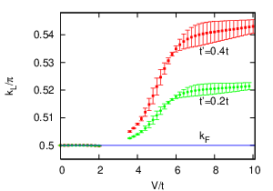
Final results for two values , , and within the whole range of parameters are shown in Fig. 5 with corresponding error bars. Presented values of in regime are calculated as described above via Eq. (8). In a window results are not shown since finite-chain calculations become unreliable due to limited wave-vector resolution and deviations from the simple finite-size scaling behavior. On the other hand, within the metallic regime , has singularity near . Therefore it makes more sense to apply instead a similar scaling analysis to the inverse values of GF, , and to locate in this way . Results obtained in this way are shown in Fig. 5 for regime . Our estimate of error bar in Fig. 5 is given as the larger value obtained either from standard deviations of parameters and or from the difference of the scaled value without taking into account the smallest system.
From Fig. 5 it is evident that at large , substantially deviates from the LSR prediction . The deviation from LSR saturates at large , whereby its value scales with the asymmetry given by . At the same time, with the decreasing and with vanishing of the MH gap , also appears to vanish. In fact, in the regime the LSR deviation seems qualitatively to follow the variation of . This is in accordance with our observation that inverse derivative () has a similar behavior to as a function of . For large , both as well as behave as , hence approaches a constant value which could be evaluated via the method of moment expansion [13]. On the other hand, the analysis of data within the metallic phase for does not show (within our accuracy) any deviation from the LSR . Hence, our results are consistent with previous confirmations of the LSR in the metallic phase away from half filling [18, 19].
In conclusion, our results clearly show that the LSR is violated in the Mott-Hubbard insulator within the 1D generalized - model where the p-h symmetry is broken via the introduction of the n.n.n. hopping . Although we concentrated only on two values of , , the behavior is quite generic whereby the violation seems to scale with the p-h asymmetry, at least for modest parameter . It should be stressed that substantially larger can perturb qualitatively the topology of the noninteracting band and which makes the interpretation more difficult. An important finding is that the violation scales as the MH gap on approaching the metallic transition at , while within the gapless (metallic) phase we do not find any evidence for the LSR violation.
Discussing possible generality of our finding, we first stress several advantages of the extended 1D - model analyzed above. Being a spinless model it allows for an accurate enough study of largest systems using the ED (compared, e.g., to the Hubbard model or multiband models), in our case up to sites. Large span of sizes then allows for a reliable finite-size scaling and extrapolation to .
Another important ingredient is the absence of a phase with a long range order in the phase diagram at . The latter is due to the 1D character of the model and supported by the exact solution at [14] which is not strongly perturbed by moderate . Thus we are dealing solely with the MH metal-insulator transition at and with its influence on the LSR. Note that in analogous models studied so far, e.g., the 2D Hubbard model on a square lattice [11, 8] or triangular lattice [13] as well as more general MH insulators [9], the MH insulator is mostly accompanied with an onset of a long-range magnetic ordering, while doped MH insulators can show ferromagnetic order etc. An appearance of the long-range order clearly spoils the translational invariance and thus the validity of the LSR [6] or at least requires the reformulation of the latter.
In view of above discussion, the studied model is just the prototype example of a model with the MH transition and one can expect that in analogy the LSR would be generally violated within the MH insulators without the p-h symmetry, even more if the MH transition is followed with an ordered state breaking the translational or some other symmetry.
Quite open question is, however, the origin of the breakdown of the LSR, or more precisely which part of the original proof [1, 2, 5] becomes invalid within the MH insulator. The basic argument [1] invokes the existence of the functional constructed via the perturbation expansion in the interaction strength. The required adiabatic connectivity [6, 9, 8] to noninteracting fermions can be clearly questioned at the metal-insulator transition which at least represents a nonanalytic point at in the extended - model, even at [14]. Moreover, it is evident that zeroes in the MH gap at the same time require divergent self energy [5, 8] which enhances doubts on the existence of an appropriate functional. The question is important in connection with the emerging conserving approximations for strongly correlated systems based on a construction of such a functional but also on dynamical-mean-field methods based on approximations for [20, 21]. In any case, a deeper understanding of the limitations of the validity of LSR is still missing and can provide new insight in the physics of strongly correlated electrons.
References
- [1] J. M. Luttinger and J. C. Ward, Phys. Rev. 118, 1417 (1960).
- [2] J. M. Luttinger, Phys. Rev. 119, 1153 (1960).
- [3] L. D. Landau, JETP 3, 920 (1956).
- [4] T. Yoshida, X. J. Zhou, D. H. Lu, S. Komiya, Y. Ando, H. Eisaki, T. Kakeshita, S. Uchida, Z. Hussain, Z.-X. Shen, et al., J. Phys.: Condensed Matter 19, 125209 (2007).
- [5] I. Dzyaloshinskii, Phys. Rev. B 68, 085113 (2003).
- [6] B. L. Altshuler, A. V. Chubukov, A. Dashevskii, A. M. Finkel’stein, and D. K. Morr, Europhys. Lett. 41, 401 (1998).
- [7] R. M. Konik, T. M. Rice, and A. M. Tsvelik, Phys. Rev. Lett. 96, 086407 (2006).
- [8] T. D. Stanescu, P. Phillips, and T.-P. Choy, Phys. Rev. B 75, 104503 (2007).
- [9] A. Rosch, Eur. Phys. J. B 59, 495 (2007).
- [10] C. Gros, K. Hamacher, and W. Wenzel, Europhys. Lett. 69, 616 (2005).
- [11] J. Kokalj and P. Prelovšek, Phys. Rev. B 75, 045111 (2007).
- [12] J. Ortloff, M. Balzer, and M. Potthoff, Eur. Phys. J. B 58, 37 (2007).
- [13] J. Kokalj and P. Prelovšek, Eur. Phys. J. B 63, 431 (2008).
- [14] J. Des Cloizeaux and M. Gaudin, J. Math. Phys. 7, 1384 (1966).
- [15] J. P. Perdew, R. G. Parr, M. Levy, and J. L. Balduz, Phys. Rev. Lett. 49, 1691 (1982).
- [16] T. Kaplan, J. Stat. Phys. 122, 1237 (2006).
- [17] R. Haydock, V. Heine, and M. J. Kelly, J. Phys. C: Solid State Physics 5, 2845 (1972).
- [18] K. B. Blagoev and K. S. Bedell, Phys. Rev. Lett. 79, 1106 (1997).
- [19] M. Yamanaka, M. Oshikawa, and I. Affleck, Phys. Rev. Lett. 79, 1110 (1997).
- [20] T. D. Stanescu and G. Kotliar, Phys. Rev. B 74, 125110 (2006).
- [21] G. Kotliar, S. Y. Savrasov, K. Haule, V. S. Oudovenko, O. Parcollet, and C. A. Marianetti, Rev. Mod. Phys. 78, 865 (2006).