Fixed points in frustrated magnets revisited

Although undoubtedly successful to describe the critical behavior of $O(N)$-like models, perturbative field theory is still unable to provide a clear, non-controversial understanding of the physics of certain more complex models among which are the famous Heisenberg or $XY$ frustrated magnets (see [1] and references therein). At the core of the problem is that different kinds of perturbative approaches, performed up to five- or six-loop order, lead to contradictory results: in dimension $d=3$, first order phase transitions are predicted within the $\varepsilon$ (or pseudo-$\varepsilon$)- expansion [2, 3, 4] whereas a second order transition is found in the fixed-dimension (FD) perturbative approaches performed either in the minimal-subtraction ($\overline{\hbox{MS}}$) scheme without $\varepsilon$-expansion [5] or in the massive scheme [6]. In fact, FD results for frustrated magnets are neither supported by experiments nor by Monte Carlo simulations [1, 7, 8, 9, 10] (see however [5] where a scaling behavior is found). They also disagree with the results obtained from the non-perturbative renormalization group (NPRG) approach [1, 11] that predicts (weak) first order phase transitions in $d=3$ in agreement with the $\varepsilon$-expansion analysis.

In this article we shed light on the discrepancies encountered in perturbative approaches to frustrated magnets by showing that the FD approaches lead to dubious predictions as for the critical physics in $d=3$. Our key-point relies on the very nature of the FD perturbative approach and is easy to grasp already for the simplest — $O(N)$ — model. In this case, the (non-resummed) renormalization group (RG) $\beta$-function at $L$ loops is a polynomial in its coupling constant $u$ of order $L+1$. Thus, it admits $L+1$ roots $u^{*}$, $\beta(u^{*})=0$, that are either real or complex. Within the $\varepsilon$-expansion, when one solves the fixed point (FP) equation in successive orders in $\varepsilon=4-d$, the only non-trivial FP retained is by definition such that $u^{*}\sim\varepsilon$. On the contrary, in the FD approaches, when one directly (analytically or numerically) solves the non-linear FP equation at fixed $d$ (fixed $\varepsilon$) no real root can be a priori discarded. As a result, the generic situation is that the number of FPs as well as their stability vary with the order $L$: at a given order, there can exist several real and stable FPs or none instead of a single one. This artefact of the FD approach is already known and was first noticed in the massive scheme in $d=3$ [12]. The way to cope with it is also known: resumming the perturbative expansion of $\beta(u)$ (see e.g. [13]) is supposed both to restore the non-trivial Wilson-Fisher FP and to suppress the non-physical or “spurious” roots. This is indeed what occurs for the $O(N)$ model for which the FP analysis performed on the resummed $\beta$-function of FD approaches enables to discriminate between physical and “spurious” FPs. However this ability of the resummation procedures to eradicate spurious solutions of the FD approach has never been questioned and, a fortiori, evaluated in the context of more complex models and, in particular, for models with several coupling constants. We precisely argue, in this article, that the situation is very different for frustrated magnets and probably for several other models. Indeed, considering the $\beta$-functions derived at five loops in the $\overline{\hbox{MS}}$ scheme and using a standard resummation procedure [5] we show that the FP found in $d=3$ without expanding in $\varepsilon$, although it persists after resummation, is in fact spurious.

Our conclusion is based on several facts: (i) the critical exponents computed at the FP supposed to control the second order behavior of frustrated magnets display bad convergence properties with the order of computation in the controversial cases of XY and Heisenberg spin systems (ii) when analyzed with the same FD approach, the field theory relevant to ferromagnetic systems with cubic anisotropy displays a similar FP — having no counterpart within the $\varepsilon$-expansion — in contradiction with its well established critical physics. The critical exponents computed at this supernumerary FP display the same bad convergence properties with the loop order as in the case of XY and Heisenberg frustrated magnets (iii) the coordinates $(u_{1}^{*},u_{2}^{*})$ of the attractive FP found in the FD approach of frustrated magnets are multivalued functions of $(d,N)$ — $N$ being the number of spin components — because of the existence of a topological singularity in the mapping between $(d,N)$ and the FP coordinates $(u_{1}^{*}(d,N),u_{2}^{*}(d,N))$. This singularity provides strong indications of the existence of pathologies in the RG equations obtained at fixed dimension (iv) finally, we provide strong arguments showing that the supernumerary FPs found in the frustrated and cubic models survive in the upper critical dimension $d=4$ where they are found to be non-Gaussian, a behavior deeply connected with the existence of the above mentioned topological singularity. Being given the present state of knowledge of $\phi^{4}$-like theories that are very likely trivial in $d=4$, this fact confirms the serious doubts on the actual existence of these supernumerary FPs.

To investigate the five-loop $\beta$ functions derived in the $\overline{\hbox{MS}}$ scheme we have to resum them. Before discussing the case of a series of two coupling constants relevant for frustrated magnets or ferromagnetic models with cubic anisotropy we recall, for the sake of clarity, the main steps needed to resum a series of one coupling constant $u$ as well as the underlying hypotheses (see for a review [14]). Let us consider a series

where the coefficients $a_{n}$ are supposed to grow as $n!$.

The Borel-Leroy sum associated with $f(u)$ is given by:

and is supposed to converge, in the complex plane, inside a circle of radius $1/a$, where $u=-1/a$ is the singularity of $B(u)$ closest to the origin. Then, using this definition as well as $\Gamma[n+b+1]=\int_{0}^{\infty}t^{n+b}\ e^{-t}dt$, one can rewrite

and, interchanging summation and integration, one can define the Borel transform of $f$ as:

In order to perform the integral in (4) on the whole real positive semi-axis one has to find an analytic continuation of $B(t)$. Several methods can be used, Padé approximants for instance. However, it is generally believed that the use of a conformal mapping is more efficient since it makes use of the convergence properties of the Borel sum. Under the assumption that all the singularities of $B(u)$ lie on the negative real axis and that the Borel-Leroy sum is analytic in the whole complex plane except for the cut extending from $-1/a$ to $-\infty$, one can perform the change of variable:

that maps the complex $u$-plane cut from $u=-1/a$ to $-\infty$ onto the unit circle in the $w$-plane such that the singularities of $B(u)$ lying on the negative axis now lie on the boundary of the circle $|w|=1$. The resulting expression $B(u(\omega))$ has a convergent Taylor expansion within the unit circle $|\omega|<1$ and can be rewritten:

where the coefficients $d_{n}(a,b)$ are computed so that the re-expansion of the r.h.s. of (6) in powers of $u$ coincides with that of (1). One obtains through (6) an analytic continuation of $B(u)$ in the whole $u$ cut-plane so that a resummed expression of the series $f$ can be written:

In practice it is interesting to generalize the expression (7) by introducing [15] the expression

whose meaning will be explained just below.

If an infinite number of terms of the series $f_{R}(u)$ were known, expression (8) would be independent of the parameters $a$ and $b$ and $\alpha$. However when only a finite number of terms are known, $f_{R}(u)$ acquires a dependence on them. In principle, the parameters $a$ and $b$ are fixed by the large order behavior of the series:

which leads to $a=a_{0}$ and $b\simeq b_{0}+3/2$ [16] while $\alpha$ is determined by the strong coupling behavior of the initial series:

which can be imposed at any order of the expansion by choosing $\alpha=\alpha_{0}$. The common assumption is that the above choice of $a$, $b$ and $\alpha$ improve the convergence of the resummation procedure since it encodes exact results.

Let us however emphasize that, often, only $a$ is known and that the other parameters, $\alpha$ and $b$, are considered either as free (as for instance in [5]) or variational (for instance in [17] where $\alpha$ is determined by optimizing the apparent convergence of the series). In any case, the choice of value of $a$, $\alpha$ and $b$ must be validated a posteriori by checking that a small change of their value does not yield strong variations of the quantities under study. Such variations would clearly indicate that one has chosen an unstable, parameter-dependent calculation procedure or that one has not computed the quantities under study at a sufficiently high order of perturbation theory to consider them as converged. In the following, we shall employ this “stability criterion” to validate – or invalidate – the results obtained by means of the FD perturbative approach to frustrated magnets.

In the context of frustrated magnets, the above described resummation procedure must be extended to several (two) coupling constants. In this case, $f$ is a function of two variables $u_{1}$ and $u_{2}$ known through its series expansion in powers of $u_{1}$ and $u_{2}$. The resummation technique used in [5] consists in considering $f$ as a function of $u_{1}$ and $z=u_{2}/u_{1}$:

and in resumming with respect to a single variable $u_{1}$ only. An important hypothesis underlying this procedure is that one can safely resum (11) with respect to $u_{1}$ while keeping $z$ fixed, i.e. without resumming with respect to $u_{2}$. Under this hypothesis the resummed expression associated with $f$ reads:

with:

where, as above, the coefficients $d_{n}(\alpha,a(z),b,z)$ in (12) are computed so that the re-expansion of the r.h.s. of (12) in powers of $u$ coincides with that of (11).

The Hamiltonian relevant for frustrated systems is given by:

where the $\kern-0.24994pt\hbox{$\phi$}\kern-5.95834pt\kern 0.50003pt\hbox{$\phi$}\kern-5.95834pt\kern-0.24994pt\raise 0.43304pt\hbox{$\phi$}_{i}$, $i=1,2$, are $N$-component vector fields and $u_{1}$ and $u_{2}$ are the coupling constants that satisfy $u_{1}>0$ and $u_{2}<4u_{1}$ — which corresponds to an Hamiltonian bounded from below. For $m^{2}>0$ the ground state of Hamiltonian (14) is given by $\kern-0.24994pt\hbox{$\phi$}\kern-5.95834pt\kern 0.50003pt\hbox{$\phi$}\kern-5.95834pt\kern-0.24994pt\raise 0.43304pt\hbox{$\phi$}_{1}=\kern-0.24994pt\hbox{$\phi$}\kern-5.95834pt\kern 0.50003pt\hbox{$\phi$}\kern-5.95834pt\kern-0.24994pt\raise 0.43304pt\hbox{$\phi$}_{2}=0$ while for $m^{2}<0$ it is given by a configuration where $\kern-0.24994pt\hbox{$\phi$}\kern-5.95834pt\kern 0.50003pt\hbox{$\phi$}\kern-5.95834pt\kern-0.24994pt\raise 0.43304pt\hbox{$\phi$}_{1}$ and $\kern-0.24994pt\hbox{$\phi$}\kern-5.95834pt\kern 0.50003pt\hbox{$\phi$}\kern-5.95834pt\kern-0.24994pt\raise 0.43304pt\hbox{$\phi$}_{2}$ are orthogonal with the same norm. The Hamiltonian (14) thus describes a symmetry breaking scheme between a disordered and an ordered phase where the $O(N)$ group of rotation is broken down to $O(N-2)$ which is relevant for frustrated magnets (for details see [1] for instance).

Let us first recall the FP structure of Hamiltonian (14) around $d=4$ at leading order in $\varepsilon=4-d$ [18, 19, 20]. For $N$ larger than a critical value $N_{c}(d)$ depending on the dimension, the RG equations display, apart the usual Gaussian ($u_{1}^{*}=u_{2}^{*}=0$) and $O(2N)$ ($u_{1}^{*}\neq 0,u_{2}^{*}=0$) FPs, two non-trivial ($u_{1}^{*}\neq 0$ and $u_{2}^{*}\neq 0$) FPs : one, $C_{+}$, is stable; the other one, $C_{-}$, is unstable. Above $N_{c}(d)$, the transition is thus predicted to be of second order. As $N$ is lowered starting from values of $N>N_{c}(d)$, the two FPs $C_{+}$ and $C_{-}$ get closer and finally collapse together for $N=N_{c}(d)$. Below $N_{c}(d)$, there is no longer a stable FP and the transition is expected to be of first order. The value of $N_{c}(d)$ for $d=3$ has been computed by several means: in a double expansion in $u_{1}$, $u_{2}$ and $\varepsilon=4-d$ up to five-loops [2, 3, 4], directly in $d=3$ in a weak-coupling expansion within the massive scheme up to six-loops [6], within a NPRG approach [1] and, finally, within the $\overline{\hbox{MS}}$ scheme without $\varepsilon$-expansion [5]. The predictions obtained within the perturbative approaches performed at fixed $d$ strongly differ from those obtained using other methods, in particular in $d\leq 3$, see below. This is the reason which led us to reconsider this kind of approach.

We thus apply the resummation procedure described above without $\varepsilon$-expansion [21] to the $\beta_{u_{i}}$ functions, $i=1,2$, obtained at five loops in the $\overline{\hbox{MS}}$ scheme [5]. More precisely, as in [5], we resum $(\beta_{u_{i}}(u_{1},z)+\varepsilon u_{i})/{u_{1}}^{2}$, $i=1,2$, instead of $\beta_{u_{i}}(u_{1},z)$, which, in fact, leads to similar results. For the model (14), the region of Borel-summability is given by $2u_{1}-u_{2}\geq 0$ (see for instance [5] for details) to which corresponds the value $a(z)=1/2$. For $2u_{1}-u_{2}\leq 0$ there exists a singularity on the positive real axis so that the series is no longer Borel-summable. However, as noted in [5], as far as $4u_{1}-u_{2}\geq 0$, the singularity of the Borel transform closest to the origin is still on the negative axis. Thus, the asymptotic behavior is still correctly taken into account by the conformal mapping and one can, a priori, trust the resummed results. Note finally that $b$ and $\alpha$ are typically varied in the ranges $[6,30]$ and $[-0.5,2]$.

One finds, in agreement with [5], that there exists a curve (parametrized by $N_{c}(d)$ or its reciprocal $d_{c}(N)$) such that for $d<d_{c}(N)$ a stable FP $C_{+}$ governs the critical properties of the system. The curves $N_{c}(d)$ obtained within this scheme is shown in Fig.1 by a dotted line ($N_{c}^{\rm FD}$). On the same figure we show the results for $N_{c}(d)$ obtained within the NPRG approach [1], red solid curve ($N_{c}^{\rm NPRG}$) and by (resummed) $\varepsilon^{5}$-expansion [5], green solid curve ($N_{c}^{\varepsilon}$). Two points must be noted. First the curves $N_{c}^{\varepsilon}(d)$ and $N_{c}^{\rm NPRG}(d)$ show a remarkable agreement being given the very different nature of the two corresponding computations. Second, one can see on Fig.1 the strong discrepancy between the two previous approaches and the perturbative FD approach. In particular the S-like shape of the curve $N_{c}^{\rm FD}(d)$ obtained within the perturbative FD approach is such that the FP $C_{+}^{\rm FD}$ exists for all $N\geq 2$ in $d=3$ contrary to the other approaches in which a FP $C_{+}$ exists only for $N>N_{c}(d=3)\simeq 5$ [1].

This situation, put together with the fact, already underlined in the Introduction, that the FD approach a priori displays spurious FPs, lead us to strongly question the validity of the results obtained at FD and, in particular, the existence of genuine FPs in $d=3$ for $N=2,3$.

We now display a specific feature of the RG flow of frustrated magnets analyzed within the FD approach that provides another strong indication of the problematic character of this approach. Let us consider the coordinates $(u_{1}^{*},u_{2}^{*})$ of the FP $C_{+}^{\rm FD}$ as functions of $d$ and $N$: $u_{i}^{*}=u_{i}^{*}(d,N)$, $i=1,2$. These functions are the roots of the $\beta$-functions of the couplings $u_{1}$ and $u_{2}$ obtained in the FD approach and resummed according to the scheme sketched above, Eq.(12):

The resummed $\beta$-functions are smooth functions of $d$ and $N$ showing no particular feature for $2<d\leq 4$ and $2\leq N<\infty$. However, as we now show, the functions $u_{i}^{*}=u_{i}^{*}(d,N)$, $i=1,2$ exhibit a non-trivial behavior as $d$ and $N$ are varied continuously around the point labelled $S$ in Fig.1.

Let us first give, in Fig.5, the precise definition of the curve $N_{c}(d)$ in the FD approach. This curve is made of two parts: the first one, labelled (I), corresponds to the part of the curve above $S$ while the second one, labelled (II), corresponds to the part below $S$. (I) is defined as the line in the $(d,N)$ plane above which there exist two non-trivial locus FP (that is having real exponents $\omega$), one stable $C_{+}^{\rm FD}$ and one unstable $C_{-}^{\rm FD}$, and below which there exists none. We recall the mechanism of disappearance of these FPs: when at fixed dimension $d$, $N$ is decreased from large values down to $N=N_{c}(d)$ the two FPs $C_{+}^{\rm FD}$ and $C_{-}^{\rm FD}$ get closer and closer from each other and finally collapse right on (I). For $N$ below $N_{c}(d)$, the coordinates $u_{1}^{*}$ and $u_{2}^{*}$ become complex and there is no longer any non-trivial FP with real coordinates. Thus, the part (I) of the curve $N_{c}(d)$ corresponds to the region where the speed of the RG flow between $C_{+}^{\rm FD}$ and $C_{-}^{\rm FD}$ vanishes. The same behavior is observed in other ($\varepsilon$-expansion and NPRG) approaches and the numerical values of $N_{c}(d)$ in the corresponding part of the curve are very close when calculated by different approches (c.f. Fig.1).

As usual, the speed of the RG flow around a FP can be obtained by linearizing the flow equations at this point. It is thus governed by the two eigenvalues of the “stability” matrix

that provide the speeds of the RG flow in its two eigendirections at the FP considered. These eigenvalues define the two critical exponents $\omega_{1}$ and $\omega_{2}$ governing the corrections to scaling. The equation of the part (I) of $N_{c}(d)$ is thus given by:

where $\omega_{1}$ is the eigenvalue of $M$ corresponding to the eigendirection of the flow joining $C_{+}^{\rm FD}$ to $C_{-}^{\rm FD}$. Now, when moving on the line $N_{c}(d)$ towards $S$ one finds that $\omega_{2}$ decreases and eventually vanishes. One thus defines the point $S$ by:

Thus, right at $S$, $\omega_{1}=\omega_{2}=0$ and, with the choice of parameters $a=1/2,b=10,\alpha=1$ one finds that at $S$, $d=3.24$, $N=7$ and $(u_{1}^{*}(S),u_{2}^{*}(S))=(0.3,0.7)$. Thus, $S$ is just outside — but not far of — the region of Borel-summability. Note also that, since its coordinates verify $4u_{1}^{*}-u_{2}^{*}>0$, $S$ is still in the region where the resummed results are trustable.

In fact, the point $S$ is also a special point in the sense that it is the endpoint of another line, labelled $(F)$ on Fig.5 which is such that below $(F)$, the two exponents $\omega_{i}$’s acquire an imaginary part and are complex conjugates: $\omega_{1}=\omega_{2}^{*}$. This means that, below $(F)$, the FPs become focuses, either attractive or repulsive. This is in particular the case of the FP $C_{+}^{\rm FD}$ found in [5] in $d=3$. From now on we concentrate on the FP $C_{+}^{\rm FD}$ since the coordinates of $C_{-}^{\rm FD}$ rapidly grow and go outside the region of Borel summability. Note that the part of (F) shown on Fig.5 lies inside the region of Borel summability and thus, within the FD approach, is supposed to be well under control.

We now define the part (II) of the curve $N_{c}(d)$ as the line separating the region where $C_{+}^{\rm FD}$ is an attractive focus FP (for $d<d_{c}(N)$) and the region where it is a repulsive focus FP (for $d>d_{c}(N)$) ¹¹ 1 The change of stability of $C_{+}^{\rm FD}$ occurs as follows. For $d<d_{c}(N)$ and $N<7.5$ and sufficiently close to (II), $C_{+}^{\rm FD}$ is a focus and is attractive inside a basin of attraction which is a limit cycle for the RG flow. This limit cycle is repulsive : inside it the RG flow converges to $C_{+}^{\rm FD}$, outside the RG flow diverges. When, at fixed $N$, the dimension $d$ is increased this limit cycle shrinks and becomes a point on (II). When $d$ is further increased, the limit cycle re-appears but now it is attractive and $C_{+}^{\rm FD}$ becomes a repulsive focus FP.. Thus, by definition, (II) is the line on which the real part of the $\omega_{i}$’s vanishes:

but it is no longer a line where $C_{+}^{\rm FD}$ collapses with another FP and disappears. It is remarkable that within the FD approach, there exists a line (the part (II) of the curve $N_{c}(d)$) that has no counterpart in other approches.

Contrary to what occurs above, the coordinates $u_{1}^{*}$ and $u_{2}^{*}$ of $C_{+}^{\rm FD}$ on the line (II) are, for a large part of (II), far outside the region of Borel summability. It is thus not possible to compute accurately the location of (II). We, however, emphasize that only the existence of (II) is necessary for the validity of our arguments, not its precise determination. As for the existence of this part (II) of the curve $N_{c}(d)$, it is an unavoidable consequence of the existence of $S$ which is supposed to be under control within the perturbative FD approach. Thus, either $S$ really exists and part (II) of $N_{c}(d)$ also exists — with a shape that could be somewhat different of the one drawn on Fig.5 — or it does not exist and neither does $S$. In this second case, this would mean that the whole resummation scheme is questionable at least for sufficiently low $d$ and $N$ (typically $d<3.2$ and $N<7$). We argue in the following that this is very probably what occurs.

Let us now show on Fig.6 that there exists a very non-trivial property of the RG flow which is a consequence of the existence of $S$. The idea is to follow continuously the coordinates of the FP $C_{+}^{\rm FD}$ along a path encircling $S$, path A in Fig.6 for instance. We start, for instance at $(d=3,N=5)$ go to $(d=3.4,N=5)$ then to $(d=3.4,N=9)$ then to $(d=3,N=9)$ and finally go back to $(d=3,N=5)$. The surprising fact is that by making a trip along such a closed path, the coordinates $(u_{1}^{*},u_{2}^{*})$ of $C_{+}^{\rm FD}$ do not go back to their original value. This is specific to $S$ since along any closed path that does not encircle this point — path B in Fig.6 for instance — the coordinates $(u_{1}^{*},u_{2}^{*})$ of $C_{+}^{\rm FD}$ always go back to their original values. Let us emphasize here that such a path can well cross part (I) of the curve $N_{c}(d)$ as path B does in Fig.6. In this case, $C_{+}^{\rm FD}$ has complex coordinates on the part of the path which is below (I), but as the path crosses again (I) the coordinates become real again and go back finally to their original values. All this makes $S$ a topological singularity of the functions $u_{1}^{*}(d,N)$ and $u_{2}^{*}(d,N)$.

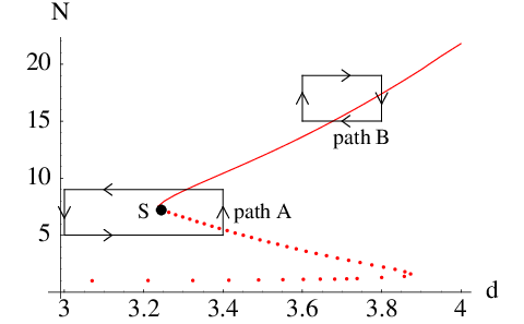
Let us remark at this stage that, before having drawn any conclusion from the existence of a topological singularity, one faces a very unusual property of the mapping from the plane $(N,d)$ to the FP coupling constants space $(u_{1}^{*},u_{2}^{*})$ which makes multivalued the functions $u_{1}^{*}(N,d)$ and $u_{2}^{*}(N,d)$. While one cannot a priori discard the possibility of such a behavior of the functions $u_{1}^{*}(N,d)$ and $u_{2}^{*}(N,d)$, it is tempting to attribute it to the coexistence at a given $(d,N)$ of FPs that are identical to those found within the $\varepsilon=4-d$ expansion and FPs that are artefacts of the FD approach. Let us now draw the full consequences of the striking behavior described above.

We now present our last argument in favor of the spurious character of the FPs obtained within the FD approach for small $d$ and $N$. It is based, to a large extent, on the existence of the singularity $S$ in the $(u_{1}^{*},u_{2}^{*})$ plane that leads to a striking property of the field theory describing frustrated magnets.

Let us first recall some basic features about the description of the long distance physics of a lattice system by a continuous field theory. The most important ingredient in this construction is the choice of a low-energy effective Hamiltonian in terms of the order parameter $\phi$. This choice implies the selection of a finite number of terms — the $\phi^{2}$ and $\phi^{4}$ terms for second order phase transitions — among the infinite number of operators obtained in the Hubbard-Stratonovitch derivation of the microscopic hamiltonian. This selection of the most relevant terms fully relies on the existence of an upper critical dimension where the theory is perturbatively infrared free, i.e. controlled by the Gaussian FP. Indeed, it is only under this condition that power-counting makes sense since it is based on the engineering dimension of the field that neglects fluctuations. Perturbation theory can then be used since, by definition, it consists in an expansion around the Gaussian theory. Also, the perturbative results obtained in this way are reliable as long as the (infrared attractive) FP found this way (i) is connected to the Gaussian by the RG flow, (ii) lies in the Borel-summability region (iii) is not too far from the Gaussian FP so that calculations performed at $L$ loops lead to converged results. Let us indicate that because of point (i) above, if the theory is trivial in $d=4$, it is very probable that any non-trivial FP identified in $d=3$, once followed continuously from $d=3$ to $d=4$, becomes Gaussian in this dimension. This is in particular what underlies the validity of the $\varepsilon=4-d$ expansion.

Let us now briefly discuss the question of triviality of scalar theories in $d=4$ and the ensuing consequences for their perturbative analysis in any dimension below 4. We first emphasize that there is no rigorous proof of the triviality of scalar theories in $d=4$. However (i) there is a large body of evidences of triviality at least for the $O(N)$ models and in particular for the Ising model (ii) it is very likely that even if the scalar models were non-trivial in $d=4$, perturbation theories would not be able to reach the corresponding FP [29]. Thus, the most natural hypothesis is that the $O(N)\times O(2)$ theory is also trivial in $d=4$. An ever weaker hypothesis, that we make and use in the following, is that this is the case when it is analyzed perturbatively. All previous considerations and assumptions lead us to conclude that, very probably, any physical FP found perturbatively in any dimension must be Gaussian when followed continuously in $d=4$. Let us notice that a non-perturbative approach, performed by some of the present authors [1] on the $O(N)\times O(2)$ theory did not lead to any non-trivial FP in $d=4$ which sustains our triviality hypotheses in $d=4$.

Therefore, according to our hypotheses, a practical way to check whether a FP found at a given dimension, $d=3$ for instance, is a genuine FP or is just an artefact of perturbation theory is to follow it by continuity up to $d=4$ [3, 30]. If the FP survives as a non-Gaussian FP at this dimension we consider it as spurious. It is important to realize that our criterion does not exclude FP in $d=3$ whose coordinates become complex between $d=3$ to $d=4$ as far as they vanish in $d=4$. This is in particular the case for all FPs associated to the paths with fixed $N$ in the $(d,N)$ plane that cross (I) above $S$.

Let us apply this criterion to analyze the FPs $P$ and $C_{+}^{\rm FD}$ that appear in the FD analysis of the cubic and frustrated models. We present our results in Fig.7 where we have displayed the coordinates $u^{*}$ and $u_{1}^{*}$ associated with these FPs as functions of $d$ at fixed $N$. Manifestly, they both survive everywhere above $d=3$ and are not Gaussian in $d=4$. In the cubic case, this is true for all values of $N$ for which $P$ exists. In the frustrated case, this is true for $N$ typically below 7. According to our criterion, $P$ is, as expected, always found to be spurious while $C_{+}^{\rm FD}$ is spurious only for $N<7$. We thus conclude, in the frustrated case, that the FPs found in $d=3$ for $N=2,3$ are spurious.

Let us emphasize that when $d$ approaches 4 the coordinates of the FPs $P$ and $C_{+}^{\rm FD}$ for $N<7$ become large and do no longer belong to the region of Borel-summability so that they cannot be determined accurately as it is the case of part (II) of the curve $N_{c}(d)$. One could thus naively conclude that it is not possible to safely decide whether these FPs are or are not Gaussian in $d=4$. This is actually not the case for at least two reasons. First, if these FPs were Gaussian in $d=4$, their coordinates just below this dimension would be extremely small and their existence as Gaussian FPs in $d=4$ could be safely established within perturbation theory even without any resummation procedure. Since for $d$ just below 4 no such FPs close to the Gaussian are found in perturbation theory, their non-Gaussian character is doubtless in $d=4$. Second, in the frustrated case, the non-Gaussian character of the $C_{+}^{\rm FD}$ FP is a clear consequence of the existence of (II) which, itself, relies on the existence of the singularity $S$. Indeed, following a FP $C_{+}^{\rm FD}$ along a path starting in $d=3$, going to $d=4$ and crossing $N_{c}^{\rm FD}(d)$ above $S$, the coordinates of $C_{+}^{\rm FD}$ become complex in $d=d_{c}(N)$ and both the real and the imaginary parts of $u^{*}_{1}$ and $u^{*}_{2}$ go to zero for $d=4$ where it is thus a Gaussian FP. If, on the contrary, the path crosses $N_{c}^{\rm FD}(d)$ below $S$, $C_{+}^{\rm FD}$ changes from a stable focus to an unstable one at $d=d_{c}(N)$ and does not go to the Gaussian in $d=4$. The singularity $S$ is therefore responsible for the non-Gaussian character of $C_{+}^{\rm FD}$ in $d=4$. Thus, even if the coordinates of $C_{+}^{\rm FD}$ for $N<7$ become large for $d$ close to 4, its non-Gaussian character in this dimension makes no doubt. Note finally that it is tempting to follow this FP $C_{+}^{\rm FD}$ above $d=4$ where there exist rigorous proofs of the triviality of the scalar $\phi^{4}$ field theory [31]. Indeed, as it is suggested by Fig.7, the FP $C_{+}^{\rm FD}$ apparently survives at finite distance above d=4. However this last fact must be taken with great caution since $C_{+}^{\rm FD}$ is now deeply out of the region of Borel-summability and one has no longer any control of where the FP really lies.

It appears from our study that the FPs $C_{+}^{\rm FD}$ identified in the FD approach are very likely spurious. The transition in frustrated magnets should thus be of — possibly weak — first order in agreement with NPRG and $\varepsilon$-expansion approaches. It remains to explain the failure in the resummation procedure used in the FD approach, Eq.(12). As already emphasized this procedure relies on the hypothesis that resumming with respect to $u_{1}$, keeping a polynomial structure in $u_{2}$, is sufficient. Alternatively, a resummation of the series with respect to the two coupling constants could be required to obtain reliable results (see for instance [32] for the randomly diluted Ising model). Postponing these considerations for a future publication [22] we assume that the use of Eq.(12) as such is justified. Then, a possible origin of the failure in the resummation procedure could be that the series considered are not known at large enough order to reach the asymptotic behavior. In this case there would be no reason to fix the parameter $a$ at its asymptotic value $a=1/2$ and one should have to vary it as $b$ and $\alpha$ to optimize the results [17]. We display in Fig.8 the curves $N_{c}^{\rm FD}(d)$ for different values of $a$. The part corresponding to large values of $N_{c}$, typically for $N_{c}\gtrsim 7$, is almost insensitive to the variations of $a$ whereas this is clearly not the case for smaller values of $N_{c}$. In particular, for sufficiently large values of $a$, typically $a\geq 1.5$, the S-like part is pushed below $d=3$ so that $N_{c}^{\varepsilon}(d)$, $N_{c}^{\rm FD}(d)$ and $N_{c}^{\rm NPRG}(d)$ are then compatible everywhere for $3<d<4$. Let us also notice in this respect that, for $a=1.3$, the shape of the curve $N_{c}^{\rm FD}(d)$ is even compatible with the results obtained in the massive scheme in $d=3$ in which one finds FPs for all values of $N$ but in the range $5.7(3)<N<6.4(4)$ [33]. This suggests that the two FD methods — massive scheme in $d=3$ and $\overline{\hbox{MS}}$ without $\varepsilon$-expansion — are in fact compatible but suffer from the same problems of convergence. Thus, under our hypothesis, all qualitative differences between the different approaches disappear, so that the problem would boil down to a question of order of computation.

Finally note that our present considerations surely pertains to the case of frustrated magnets in $d=2$ [34]. Indeed we have checked that the FP found in $d=2$ is continuously related to the FP $C_{+}^{\rm FD}$ in $d=3$ which makes its existence doubtful. Our conclusions could also apply in other situations where FPs that have no counterpart in the $\varepsilon$-expansion are found, as it is the case, for instance, in QCD at finite temperature [35].

We wish to thank P. Azaria, P. Calabrese, R. Folk, R. Guida and J. Zinn-Justin for useful discussions. Work of Yu.H. was supported in part by the Austrian Fonds zur Förderung der wissenschaftlichen Forschung, Project P19583. We acknowledge the CNRS-NAS Franco-Ukrainian bilateral exchange program.

References

- [1] Delamotte B, Mouhanna D and Tissier M 2004 Phys. Rev. B 69 134413
- [2] Antonenko S A, Sokolov A I and Varnashev K B 1995 Phys. Lett. A 208 161
- [3] Holovatch Yu, Ivaneyko D and Delamotte D 2004 J. Phys. A 37 3569
- [4] Calabrese P and Parruccini P 2004 Nucl. Phys. B 679 568
- [5] Calabrese P, Parruccini P, Pelissetto A and Vicari E 2004 Phys. Rev. B 70 174439
- [6] Pelissetto A, Rossi P and Vicari E 2001 Phys. Rev. B 63 140414(R)
- [7] Itakura M 2003 J. Phys. Soc. Jap. 72 74
- [8] Peles A, Southern B W, Delamotte B, Mouhanna D and Tissier M 2004 Phys. Rev. B 69 220408(R)
- [9] Bekhechi S, Southern B, Peles A and Mouhanna D 2006 Phys. Rev. E 74 016109
- [10] Quirion G, Han X, Plumer M L and Poirier M 2006 Phys. Rev. Lett. 97 077202
- [11] Tissier M, Delamotte B and Mouhanna D 2000 Phys. Rev. Lett. 84 5208
- [12] Parisi G 1980 J. Stat. Phys. 23 49
- [13] Zinn-Justin J 1989 Quantum Field Theory and Critical Phenomena 3rd ed (New York: Oxford University Press)
- [14] Suslov I M , 2005 J.Exp.Theor.Phys. 100 1188
- [15] Kazakov D I, Tarasov O V and Shirkov D V 1979 Theor. Math. Phys. 38 15
- [16] Le Guillou J C and Zinn-Justin J, 1980 Phys. Rev. B 21 3976
- [17] Mudrov A I and Varnashev K B 1998 Phys. Rev. E 58 5371
- [18] Garel T and Pfeuty P 1976 J. Phys. C: Solid St. Phys. 9 L245
- [19] Bailin D, Love A, and Moore M A J. Phys. C: Solid State Phys. 10 1159
- [20] Yosefin M and Domany E 1985 Phys. Rev. B 32 1778
- [21] Schloms R and Dohm V 1987 Europhys. Lett. 3 413
- [22] Delamotte B, Holovatch Yu, Ivaneyko D, Mouhanna D and Tissier M 2006 unpublished
- [23] Folk R, Holovatch Yu and Yavors’kii T 2000 Phys. Rev. B 62 12195 err. ibid. 63, 189901 (2001)
- [24] Kleinert H and Schulte-Frohlinde V 1995 Phys. Lett. B 342 284
- [25] Carmona J M, Pelissetto A and Vicari E 2000 Phys. Rev. B 61 15136
- [26] Calabrese P, Pelissetto A and Vicari E 2003 Phys. Rev. B 67 024418
- [27] Tissier M, Mouhanna D, Vidal J and Delamotte B 2002 Phys. Rev. B 65 140402
- [28] Itakura M, 1999 Phys. Rev. B 60 6558
- [29] Callaway D J E, 1988 Phys. Rep. 167 241
- [30] Dudka M, Yu Holovatch and Yavors’kii T 2004 J. Phys. A 37 10727
- [31] Aizenmann M, 1981 Phys. Rev. Lett. 47 1
- [32] Alvarez G, Martìn-Mayor V and Ruiz-Lorenzo J J 2000 J. Phys. A 33 841
- [33] Calabrese P, Parruccini P and Sokolov A I 2003 Phys. Rev. B 68 094415
- [34] Calabrese P, Parruccini P and Sokolov A I 2002 Phys. Rev. B 66 180403(R)
- [35] Basile F, Pelissetto A and Vicari E 2005 JHEP 0502 044