Keywords: Carbon-carbon plain weave composites, homogenization, periodic unit cell, Mori-Tanaka method, orientation averaging
Effective Properties of Textile Composites: Application of the Mori-Tanaka Method
Abstract
An efficient approach to the evaluation of effective elastic properties of plain weave textile composites using the Mori-Tanaka method is presented. The method proves its potential even if applied to real material systems with various types of imperfections including the non-uniform waviness of the fiber-tow paths, both along its longitudinal direction and through the laminate thickness. Influence of the remaining geometrical parameters is accounted for by optimal calibration of the shape of the equivalent ellipsoidal inclusion. An application of the method to a particular sample of the carbon-carbon composite laminate demonstrates not only its applicability but also its efficiency particularly when compared to finite element simulations.
1 Introduction
Plain weave composites, reinforced by mutually interlaced systems of unidirectional fiber tows bonded to a matrix, belong to a progressive material systems with widespread applications in virtually all areas of engineering. As a particular example, consider carbon-carbon (C/C) composites, originally developed for the space and automobile industry, which now find uses in the medicine owing to their appealing biological compatibility with a living soft tissue, e.g. [Pesakova:2003:BBP]. A proper characterization of these material systems, especially from the mechanical response point of view, thus appears rather important.
While a detailed two-dimensional (2D) analysis of a heat conduction problem for the evaluation of effective (macroscopic) thermal conductivities seems to be sufficient, e.g. [Tomkova:2006, Tomkova:2008:EETC], a reliable estimate of the mechanical response of such systems requires in general a solution of a full three-dimensional (3D) problem. This task, however, presents a significant challenge even if limiting our attention to a linear elastic behavior. Not only the characteristic 3D structure of textile composites, but also various types of imperfections in woven path developed during the manufacturing process preclude a direct formulation of a simple computational model.
A considerable research effort has been invested in the last two decades into providing a simple yet accurate scheme for the predictions of macroscopic elastic properties of woven composites. With an increasing level of sophistication, these models include modified rule of mixtures, approaches based on classical laminate theories (CLT) and detailed three-dimensional finite element method (FEM) based simulations, see e.g. [Cox:1997:HAMTC, Chung:1999:WFC, Takano:1999:HMTC, Lomov:2007:MFEM] for a review and comparison of individual approaches. The latter class of computational models is considered to be the most accurate one particularly if combined with concise geometrical data [Barbero:2006:FEM, Zeman:2004:RC, Lomov:2007:MFEM].
The FEM simulations show, however, certain disadvantages. Perhaps the most critical one is a relatively high computational cost due to laborious preparation of finite element meshes. Moreover, to incorporate at least the dominant microstructural imperfections observed in real systems into the FEM model is far from being trivial and deserves a special treatment typically based on an appropriate statistical characterization [Zeman:2004:RC, Zeman:MSMSE:2007]. The CLT approaches are, on the other hand, easy to implement and provide a reasonable approximation of the in-plane elastic moduli. However, since this class of models approximates the composite as a coupling of serial and parallel laminates stacked to resemble the actual geometry, it becomes inadequate when predicting the out-of-plane response. Therefore, a procedure offering a reasonable compromise between the accuracy of FEM-based modeling and simplicity of traditional CLT methods is still on demand.
In the last decade, effective media theories, widely used in continuum micromechanics [Bohm:2005:SIBA], have been recognized as an attractive alternative to CLT-based methods. Such an approach was pioneered by ? and ?, who modeled knitted composites as an assembly of spherical fibers in an isotropic matrix and used the Mori-Tanaka (M-T) method [Mori:1973:MTM] to evaluate the overall response. Further advancements in the field include the Transformation Field Analysis approach due to ? and the work of ? in the framework of the theory of periodic eigenstrains. All these studies report good correspondence with experimental data with an error comparable to experimental scatter. Moreover, with regard to imperfect textiles, the Mori-Tanaka method appears particularly useful as it allows, through the application of orientation averaging techniques, see e.g [Yushanov:1998:STCM, Gommers:1998:MTMATC, Schjodt-Thomsen:2001:MT, Duschlbauer:2003:MTB, Jing:2003:MESF, Doghri:2006:MIE, and references therein], for a direct introduction of imperfections in the fiber-tow path represented here by histograms of distribution of the fiber-tow orientation angles. It is worth noting that such histograms, when constructed for all plies in the laminate, also reflect, at least to some extent, tow path imperfections due to inter-layer shift typical for real material systems displayed in Figure 1(a),(b).
A successful application of the M-T method for the prediction of the effective material parameters of textile composites including the above knowledge of the actual microstructure requires, however, completion of the following tasks:
- •
Quantification of the real micro (meso) structure through a detailed evaluation of images of real material samples. This part of the analysis is briefly addressed in Section 2 for a C/C composite specimen.
- •
The basic geometrical information are then used to construct an idealized three-dimensional periodic unit cell exploiting the geometrical model proposed by ?. Such a unit cell serves as a point of departure for a subsequent application of the M-T method. Review of the model together with essential steps of the FEM based simulations using the first-order homogenization technique is provided in Section 3.
- •
Formulation of the Mori-Tanaka method is then presented in Section 4 with emphasis given to the symmetry of the overall material stiffness matrix and capturing interaction between individual tows. It is shown that special care is required when replacing the actual fiber tow by an equivalent ellipsoidal inclusion. In the present formulation, the shape of the equivalent ellipsoid is thus treated as an internal parameter of the method determined by matching the M-T estimates with the results derived in Section 3.
- •
Two possible approaches to the calibration of the internal parameters of the method are considered. In the first variant, the optimal ellipsoidal shape is found by matching directly the results of the finite element simulations, executed on a “training” set reflecting the in-situ determined scatter of geometrical parameters. It is worth noting that such procedure allows us to introduce possible deviations from the “ideal” (average) geometry of the textile structure presented in Section 2. The second approach employs the finite element data at hand to propose a simple relation between basic parameters of the textile composite and parameters of the optimal ellipsoid. Section 5 is concluded by verification and validation of the developed heuristics.
- •
Once the shape of the ellipsoid is calibrated, the orientation averaging can be used in conjunction with the histograms of the fiber-tow orientation angle. This final step leading to estimates of the overall elastic response of imperfect C/C textile composites is examined in Section 6. Section 7 then summarizes the final results and offers possible extensions particularly with account to intrinsic porosity of these material systems.
In the following text, the Voigt representation of symmetric tensorial quantities is systematically employed, e.g. [Bittnar:1996:NMM]. In particular, , and denote a scalar value, a vector or a matrix representation of a second-order tensor and a matrix representation of a fourth-order tensor, respectively. Other symbols and abbreviations are introduced in the text as needed.
2 Microstructure evaluation
As already mentioned in the introductory part, obtaining reliable predictions of the effective mechanical properties of textile composites requires a thorough analysis of their actual microstructure. Figure 1(a) shows a particular C/C composite laminate consisting of eight layers of carbon fabric Hexcel G 1169 bonded to a carbon matrix. A total of twenty such specimens having dimensions of mm were fixed into the epoxy resin and after curing subjected to final surface grounding and polishing using standard metallographic techniques to produce specimens suitable for the subsequent image analysis.

While image analysis software LUCIA G might be used directly to process the actual image of the specimen in Figure 1(a), it proves more advantageous, owing to a low color contrast of the carbon reinforcement and carbon matrix, to collect the necessary geometrical information from its binary counterpart plotted in Figure 1(b). Several such sections taken from various locations of the laminated plates were examined to obtain basic statistics of various parameters including segment dimensions, fiber tow thickness, shape of the fiber tow cross-section, etc. The resulting values are stored in the second column of Table 1. The averages of basic geometrical data were finally used to construct an equivalent or rather an ideal periodic unit cell (EPUC) appearing in Figure 1(c,d) employing the description due to ?. The three-dimensional geometric model is defined by four parameters: the tow wavelength , the tow height , tow spacing and the layer thickness , cf. Figure 1(c).
| Carbon/Carbon | E-glass/Vinylester | E-glass/Epoxy | |
| Parameter | ? | ? | ? |
| [m] | 2,250 155 | 1,200 | 620 |
| [m] | 300 50 | ||
| [m] | 150 20 | 50 | 100 |
| [m] | 400 105 | 20 | 20 |
| [] | 53.2 1.8 | 79.8 | 69.7 |
Note, however, that the real composite shows a number of imperfections which certainly should not be completely disregarded. It will be seen later in Section 4 that the nonuniform waviness and to some extent also the fiber inclinations due to production-related mutual shift of individual layers clearly visible in Figure 1(b) can be accounted for by utilizing histograms of inclination angles derived from centerlines of individual fiber tows, see Figure 1(e,f) and [Vopicka:2004:PGV] for more details. The idealized geometry in Figure 1(c) assumes, nevertheless, the centerlines of the warp and fill systems of tows in a simple trigonometric form [Kuhn:1999:MPWCG]
| (1) |
3 Periodic unit cell analysis
Having quantified the real microstructure, the resulting EPUC can be readily employed to provide FEM estimates of the required effective moduli. This particular step of the proposed analysis scheme will now be briefly reviewed.
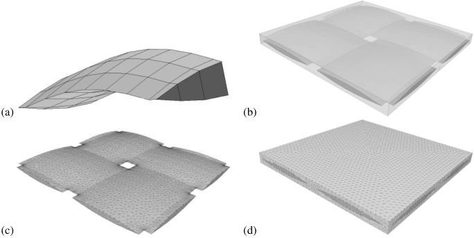
To that end, consider an EPUC in Figure 1(d) with the local coordinate system defined such that the local axis is aligned with the fiber tow direction. Definitely the most tedious step in the entire analysis is preparation of a three-dimensional finite element mesh complying with the periodic boundary conditions (the same positions of the element nodes on the opposite faces of the cell). Here, the elements of CAD operations combined with volumetric modeling capabilities of ANSYS package are used to generate the finite element mesh employing the mapped meshing technique discussed by ? and ?.
In order to ensure symmetry of the resulting FEM mesh, a primitive block of the tow shown in Figure 2(a) is modeled first. Next, using mirroring, copying and merging operations, the whole volume of one reinforcement layer is generated. Finally, the volume corresponding to the matrix phase is generated by subtracting the body of reinforcements from the matrix as depicted in Figure 2(b). To reflect the required periodicity only one of the two opposite faces is meshed using the advancing front technique and then copied to the associated one. At last, the tetrahedral elements corresponding to tows and matrix are generated based on the data created in the previous steps, leading to finite element meshes shown in Figure 2(c,d).
The further numerical treatment now proceeds as follows, cf. [Michel:1999:EPC]. Suppose that the periodic unit cell in Figure 2(d) is loaded by a macroscopic strain vector . In view of the assumed microstructure periodicity, the local displacement field then admits the following decomposition
| (2) |
where represents a periodic fluctuation of due to the presence of heterogeneities and matrix stores the coordinates of . The local strain then assumes the form
| (3) |
where the fluctuating part vanishes upon the volume averaging. Next, introducing Equation (3) into the principle of virtual work (the Hill-Mandel lemma) yields
| (4) |
where stands for the volumetric averaging with respect to the PUC and is used to denote a quantity in the local coordinate system. The local stress field then reads
| (5) |
where is the material stiffness matrix. Relating the strains in the local and global coordinate systems by the well-known relations , , see e.g. [Bittnar:1996:NMM], and inserting Equation (5) into Equation (4) yields the stationarity conditions in the form
| (6) |
to be satisfied for all kinematically admissible variations .
The homogenized stiffness matrix follows from post-processing of the solution of six independent elasticity problems, discretized using conforming FEM procedure, see [Zeman:2003:ACM, Zeman:2004:RC] for further details. In particular, each column of coincides with the volume averages of local stress resulting from a macroscopic strain with one component set to one and with the remaining entries equal to zero.
4 Application of the Mori-Tanaka to woven composites
4.1 Overall stiffness of composite with non-aligned inclusions
Consider an -phase composite with an isotropic matrix phase having the stiffness matrix and being reinforced with families of ellipsoidal heterogeneities. Each heterogeneity is characterized by the stiffness matrix and occupies a volume . With reference to [Benveniste:1991:ODES], the Mori-Tanaka estimate of the overall stiffness matrix then reads
| (7) |
where denotes the volume fraction of the -th phase. The corresponding partial strain concentration factor has the form
| (8) |
where the matrix is provided by
| (9) |
Function is related to Green’s function of an infinite medium with stiffness matrix (see, e.g. [Castenada:1995:ESD, Section 3.1] for more details). It follows from the celebrated work of ? that for ellipsoidal inclusions, is constant and can be evaluated as
| (10) |
where is the Eshelby matrix. When the matrix phase is isotropic, explicit expressions for can be found in, e.g. [Eshelby:1957:SFI, Mura:1982:MDS].
While the M-T model has proved itself to be accurate for composites reinforced either by randomly oriented or aligned inclusions with an identical shape, in general case it may lead to a non-symmetric stiffness matrix , see e.g. [Benveniste:1991:ODES, Ferrari:1991:AHL, Castenada:1995:ESD] for the in-depth discussion. In this work, a simple re-formulation proposed by ? is employed to preserve the overall symmetry of the stiffness matrix using the orientation averaging.
To this end, we approximate the material system under investigation as a two-phase composite () consisting of an isotropic matrix () and with index collectively denoting the reinforcing tow phase, composed of heterogeneities of identical shape but different orientations.11 1 Therefore, the employed geometrical data reduce to the volume fraction of one of the phases and appropriate quantification of orientation distribution. Suppose for a moment aligned heterogeneities . Then, the overall stiffness matrix is symmetric [Benveniste:1991:ODES] and can be decomposed to
| (11) |
Notice that due to assumed isotropy of the matrix phase, the matrix is independent of the reference coordinate system while stores the orientation-dependent part. Following [Schjodt-Thomsen:2001:MT], the estimate of the overall stiffness of a composite reinforced with non-aligned heterogeneities is provided by
| (12) |
where the double brackets denote averaging over all possible orientations. In particular, when the orientation of each heterogeneity is parametrized in terms of the Euler angles and , see Figure 3,22 2 Note that so-called ” convention” is used; i.e. a conversion into a new coordinates system follows three consecutive steps. First, the rotation of angle around the original axis is done. Then, the rotation of angle around the new axis is followed by the rotation of angle around the new axis to finish the conversion. the orientation-dependent part can be expressed as
| (13) |
where the explicit expression of the transformation matrix can be found in e.g. [Schjodt-Thomsen:2001:MT] and [Zeman:2003:ACM, Appendix A].
The orientation average then follows from
| (14) |
with denoting the joint probability density describing the distribution of individual angles.
4.2 Application to plain weave composites with ideal geometry
To examine the theoretical formulation presented in the previous Section, consider again an ideal plain weave textile composite already studied in Section 3. In this particular case, the joint probability density function results from the harmonic shape of the centerline, recall Equation (1). Applying the change of variable formula [Rektorys:1994:SOM, Section 33.9], we obtain after some algebra the expression of the probability density in the form
where
Equation (14) then becomes
| (15) |
and similarly for the fill system we get
| (16) |
Following Equation (12), the resulting homogenized stiffness matrix of a plain weave composite then reads
| (17) |
where the averages of the basic geometrical parameters and the material parameters of the two-phase composite including the volume fraction of individual phases are assumed to be known quantities. The matrices and implicitly depend, however, on the Eshelby matrix , which is yet to be determined.
| Carbon/Carbon | E-glass/Vinylester | E-glass/Epoxy | |
|---|---|---|---|
| ? | ? | ||
| Matrix | |||
| [GPa] | 30 | 3.4 | 3.12 |
| 0.19 | 0.35 | 0.38 | |
| Fiber tow | |||
| [GPa] | 210 | 58.397 | 51.352 |
| [GPa] | 86 | 8.465 | 5.342 |
| [GPa] | 72 | 20.865 | 15.040 |
| [GPa] | 27.7 | 7.527 | 5.342 |
| 0.27 | 0.241 | 0.262 |
To take advantage of the closed-form Eshelby solution [Eshelby:1957:SFI], it will be assumed that the actual shape of the fiber tow can be well represented by an equivalent ellipsoid with semi axes . Then, the accuracy of the M-T method is governed by a proper choice of the semi-axes as exemplified by the following case study. In particular, three representations is considered: (i) a spherical shape , (ii) a cylindrical shape and (iii) an ellipsoid . The unit cell with average geometrical parameters appearing in the second column of Table 1 and the constituent properties stored in the second column of Table 2, i.e. C/C composite system, are considered. Note that in order to achieve the maximum phase stiffness contrast, the tow parameters shown in Table 2 correspond to the pure carbon fibers. The corresponding homogenized stiffness matrix entries are stored in Table 3 together with the FEM data.
| Method | ||||||
|---|---|---|---|---|---|---|
| [GPa] | [GPa] | [GPa] | [GPa] | [GPa] | [GPa] | |
| FEM (Ideal geometry) | 89.94 | 16.55 | 14.06 | 48.67 | 20.26 | 41.53 |
| M-T (Spherical inclusion) | 64.73 | 14.57 | 14.85 | 54.56 | 24.17 | 28.71 |
| M-T (Cylindrical inclusion) | 103.6 | 16.15 | 15.55 | 52.74 | 23.99 | 28.75 |
| M-T (Ellipsoidal inclusion) | 88.35 | 16.85 | 14.94 | 50.24 | 21.54 | 41.19 |
Clearly, comparing the M-T estimates with FEM based results allows us to draw the following two conclusions: (i) the Mori-Tanaka method appears as a reliable alternative to the first-order periodic homogenization based on the finite element method, (ii) the choice of the Eshelby matrix can hardly be made arbitrarily. It should be noted that the illustrative results correspond to volume fraction , for which the accuracy of the Mori-Tanaka method typically deteriorates. Therefore, the optimal ellipsoid not only accounts for the tow geometry, but also for approximately captures tow interactions due to non-dilute volume fractions of the reinforcing phase.
5 Optimal shape of equivalent ellipsoid
5.1 FEM-based calibration
The essential goal now becomes to find the optimal shape of the ellipsoid by matching the FEM results with the M-T predictions for C/C material system. To take into account the observed uncertainties in the textile geometry, a collection of PUCs, rather than a single one, is used for the calibration. To generate such a set we exploit the scale-invariance of the first order homogenization and set . The remaining parameters were generated using the Latin Hypercube Sampling method [Iman:1980:SSS], assuming uniformly distributed random variables with the statistics stored in the second column of Table 1. Twenty such unit cells were generated and subject to the FEM-based homogenization procedure, yielding the homogenized stiffnesses listed in Table 4.
| Statistics | ||||||
|---|---|---|---|---|---|---|
| [GPa] | [GPa] | [GPa] | [GPa] | [GPa] | [GPa] | |
| Average | 86.96 | 16.00 | 13.65 | 47.73 | 19.78 | 39.13 |
| Standard deviation | 2.29 | 0.40 | 0.30 | 0.68 | 0.34 | 1.87 |
| Optimized M-T (ideal geometry) | 88.81 | 16.13 | 13.89 | 47.35 | 20.17 | 40.40 |
| Optimized M-T (training set) | 88.23 | 16.78 | 14.94 | 49.09 | 20.09 | 40.26 |
Since the Eshelby matrix depends on the mutual ratio of the ellipsoid semi-axes only, it is possible to set , which leaves us with only two parameters undetermined. To characterize the discrepancy between the FEM and M-T solution, the following error measure is introduced
| (18) |
When PUCs are considered, the objective function assumes the form:
| (19) |
where the superscript represents the -th member in the training set. The optimal shape characterized by and can be then found from the minimization procedure
| (20) |
A graphical representation of the objective function assuming a single (average) periodic unit cell is plotted in Figure 4 for the sake of illustration.
Note that the explicit expression of the Eshelby matrix is not available in this particular case, which essentially precludes the use of classical gradient-based optimization algorithms. The stochastic optimization methods, on the other hand, appear to be a more appropriate choice. The particular algorithm, based on the surrogate function model combined with evolutionary algorithm adopted in the present study is briefly described in A.
The solution of the optimization problem then yields the optimal values of semi-axes and with the optimal value . It is worth noting that the optimum compares rather well with the case when the minimization is performed with respect to the ideal unit cell only, for which , see also Table 4 for a comparison in terms of stiffness matrix entries. This confirms the predictive capabilities of the M-T approach, at least in the range of addressed geometrical variations.
5.2 Heuristic calibration
Although the advocated M-T approach seems to offer an efficient way to the prediction of the homogenized properties, especially when handling composites with random tow imperfections, cf. Section 6, it still requires the reference FEM simulations to tune the Eshelby matrix. Therefore, it appears advantageous to establish a heuristic link between the EPUC parameters and optimal ellipsoidal shape. In previous works [Gommers:1998:MTMATC, Huysmans:1998:PIA], such a relation was derived from the local centerline curvature and calibrated using selected elastic constants. The current framework, on the other hand, offers a possibility to systematically use information contained in the previously generated set of EPUCs.
In the first step of the analysis, the optimization procedure is executed independently for each EPUC (i.e. with objective function (18)), yielding a set of optimal parameters . Subjecting the results to correlation analysis, see e.g. [Rektorys:1994:SOM, Section 34.5], reveals that the parameter is strongly correlated with ratio (with the coefficient of correlation equal to ), while it is almost independent of value. An analogous trend can be observed between and parameter. Such results authorize us to postulate a simple linear relation between the optimal ellipsoid shape and EPUC parameters. The optimal fit, now determined using objective function (20), finally leads to a semi-empirical formula
| (21) |
No doubt, such heuristics still builds on a representative finite element simulations and as such requires to be verified and validated against independent data. In the current work, we examine two plain weave composite systems thoroughly analyzed in [Barbero:2005:MFRC, Barbero:2006:FEM]: (i) E-glass/Vinylester composite [Scida:1999:MM3D], (ii) E-glass/Epoxy material system [Kollegal:2000:SMP]. The corresponding geometrical data are stored in Table 1, while the material parameters of individual constituents are available in Table 2. It is worth noting that the considered material systems offer a considerably different tow volume fractions and elastic constants of individual phases than in the calibration step. Moreover, to keep the validation objective, the comparison will now be based on orthotropic engineering moduli (see, e.g. [Bittnar:1996:NMM]) rather than stiffness matrix entries.
| E-glass/Vinylester | E-glass/Epoxy | ||||||
|---|---|---|---|---|---|---|---|
| Experiment | PMM | FEM | M-T | Experiment | PMM | M-T | |
| [GPa] | 24.8 1.1 | 25.1 | 24.5 | 25.8 | 19.29 | 18.9 | 19.2 |
| [GPa] | 8.5 2.6 | 10.5 | 10.3 | 12.4 | 8.74 | 8.83 | |
| [GPa] | 4.2 0.7 | 2.91 | 3.16 | 4.08 | 2.57 | 2.92 | |
| [GPa] | 6.5 0.8 | 4.37 | 5.52 | 6.44 | 3.18 | 3.07 | 3.85 |
| 0.28 0.07 | 0.34 | 0.38 | 0.38 | 0.44 | 0.46 | ||
| 0.1 0.01 | 0.12 | 0.13 | 0.14 | 0.2 | 0.13 | 0.13 | |
For the E-glass/Vinylester composite, performance of the M-T method is compared with the Periodic Microstructure Model (PMM) (an alternative micromechanics-based method based on a detailed geometrical model due to ?), independent finite element study in ANSYS and experimental data. Results of the comparison, reported in Table 5, demonstrate a reasonable match between the M-T predictions and remaining values. Although the accuracy of the Young moduli is somewhat inferior with respect to detailed models, the shear behavior is predicted very well and also the values of the Poisson ratios are consistent with the results of alternative numerical approaches.
Similar conclusions can be made for the E-glass/Epoxy textile system, see Table 5, where even closer match between the detailed numerical model can be observed. In overall, the presented data provide an evidence that the heuristic relation (21) leads to reasonably accurate estimates of the homogenized elastic properties.
6 Application to real geometry of C/C composite system
Having identified the optimal form of the Eshelby matrix, the attention is now focused again on the general formulation and the orientation averaging in particular, recall Equation (14). Unlike in Section 4.2, however, the joint probability density function is represented by real histograms of the fiber tow orientation angles already introduced in Figure 1(f); see also Figure 5 for additional examples. With such probabilistic characterization in hand, the warp stiffness can be estimated as, cf. Equation (15),
| (22) |
where denotes the number of sampling values and the discrete angles and probabilities follow directly from the image analysis data. The rest of the analysis exactly duplicates the perfect unit cell case.
The complete data from the analyzed C/C sample involve eleven such histograms describing the waviness of the fiber tow in individual plies. The final homogenized properties together with the elementary statistical characterization are summarized in Table 6.
| Histogram | ||||||
|---|---|---|---|---|---|---|
| [GPa] | [GPa] | [GPa] | [GPa] | [GPa] | [GPa] | |
| 1 | 86.94 | 16.71 | 15.30 | 50.28 | 21.63 | 42.81 |
| 2 | 88.19 | 17.16 | 15.64 | 51.15 | 22.23 | 44.27 |
| 3 | 88.34 | 17.14 | 15.67 | 51.20 | 22.24 | 44.49 |
| 4 | 86.73 | 16.64 | 15.24 | 50.11 | 21.49 | 42.58 |
| 5 | 86.25 | 16.47 | 15.11 | 49.45 | 21.27 | 42.02 |
| 6 | 86.57 | 16.58 | 15.20 | 49.99 | 21.63 | 42.39 |
| 7 | 88.52 | 17.28 | 15.72 | 51.35 | 22.35 | 44.69 |
| 8 | 90.26 | 17.90 | 16.20 | 52.59 | 23.23 | 46.71 |
| 9 | 86.11 | 16.42 | 15.07 | 49.69 | 21.21 | 41.83 |
| 10 | 86.82 | 16.67 | 15.26 | 50.17 | 21.54 | 42.68 |
| 11 | 87.96 | 17.07 | 15.58 | 51.00 | 22.15 | 43.98 |
| Average | 87.52 | 16.91 | 15.45 | 50.63 | 21.91 | 43.49 |
| Standard deviation | 1.26 | 0.44 | 0.34 | 0.91 | 0.60 | 1.48 |
It becomes clear by associating the results in Table 6 with the corresponding micrographs that those segments which have more fibers oriented near the direction provide a stiffer response than the others. As an illustration, consider e.g. histograms No. and in Figure 5 and corresponding stiffnesses in Table 6. Nevertheless this difference is, due to a rather narrow range of the inclination angles, not too important, especially if concerning the approximate character of the M-T method.
7 Conclusions
In the present work, an efficient numerical method for the homogenization of plain weave composites with both ideal and imperfect tow paths based on the Mori-Tanaka method has been proposed. The adopted strategy builds on the matching of results of the detailed FEM analysis with the micromechanical model. The most pertinent conclusions can be stated as follows:
- i)
The simplified method is able to deliver the homogenized parameters with values comparable with the detailed finite element simulations. The resulting method compares well with independent numerical approaches and available experimental data.
- ii)
The accuracy of the method depends on the shape of an equivalent ellipsoid, which represents both geometrical and mechanical effects, such as inter-tow interactions. The parameters of the inclusion follow from a well-defined global optimization problem and a FEM-generated training set. Moreover, the optimal shape is robust with respect to moderate geometry perturbations.
- iii)
The method allows us to directly assess the effects of tow waviness quantified by histograms of inclination angles, including the statistical characterization of the homogenized stiffnesses.
The future extension of the method will include the treatment of the intrinsic porosity of the C/C composite evident from Figure 1(a). In the framework of multi-phase Mori-Tanaka approaches, the porosity can be modeled as an additional phase characterized in the simplest case by volume fractions or by three-dimensional computer tomography data, see [Piat:2006:MMCVI_1, Piat:2006:MMCVI_2] for related studies. Such work is in progress and will be reported separately.
Acknowledgments
Authors would like to thank Jan Vorel for helpful discussions on the subject. The financial support provided by the GAČR grant No. 106/07/1244 and partially also by the research project CEZ MSM 6840770003 is gratefully acknowledged.
References
References
- [2] [] Bahei-El-Din Y A, Rajendran A M & Zikry M A 2004 Int. J. Solids Struct. 41(9–10), 2307–2330.
- [4] [] Barbero E J, Damiani T M & Trovillio J 2005 Int. J. Solids Struct. 42(9–10), 2489–2540.
- [6] [] Barbero E J, Trovillion J, Mayugo J A & Sikkil K K 2006 Compos. Struct. 73(1), 41–52.
- [8] [] Benveniste Y, Dvorak G & Chen T 1991 J. Mech. Phys. Solids 39(7), 927–946.
- [10] [] Bittnar Z & Šejnoha J 1996 Numerical methods in structural mechanics ASCE Press and Thomas Telford, Ltd New York and London.
- [12]
[]
Böhm H 2005 A short introduction to basic aspects of continuum
micromechanics Technical Report hjb/ILSB 050103 Christian Doppler
Laboratory for Functionally Oriented Materials Design, Institute of
Lightweight Design and Structural Biomechanics, Vienna University of
Technology.
*#1 - [14] [] Chung P & Tamma K 1999 Int. J. Numer. Methods Eng. 45(12), 1757–1790.
- [16]
[]
Cox B & Flanagan G 1997 Handbook of analytical methods for textile
composites NASA Contractor Report 4750 Langley Research Center.
*#1 - [18] [] Doghri I & Tinel L 2006 Comput. Meth. Appl. Mech. Eng. 195(13–16), 1387–1406.
- [20] [] Duschlbauer D, Pettermann H & Böhm H 2003 Scr. Mater. 48(3), 223–228.
- [22] [] Eshelby J 1957 Proc. R. Soc. A-Math. Phys. Eng. Sci. 241, 376–396.
- [24] [] Ferrari M 1991 Mech. Mater. 11(3), 251–256.
- [26] [] Gommers B, Verpoest I & Van Houtte P 1998 Acta Mater. 46(6), 2223–2235.
- [28] [] Huysmans G, Verpoest I & Van Houtte P 1998 Acta Mater. 46(9), 3003–3013.
- [30] [] Ibrahimbegovic A, Knopf-Lenoir C, Kučerová A & Villon P 2004 Int. J. Numer. Methods Eng. 61(14), 2428–2460.
- [32] [] Iman R & Conover W 1980 Commun. Stat.-Theory Methods 9(17), 1749–1842.
- [34] [] Jing X N, He L H & Zhao J H 2003 Model. Simul. Mater. Sci. Eng. 11(1), 11–19.
- [36] [] Kollegal M G & Sridharan S 2000 J. Compos Mater. 34(20), 1756–1786.
- [38] [] Kuhn J L & Charalambides P G 1999 J. Compos Mater. 33(3), 188–220.
- [40] [] Kučerová A, Lepš M & Skoček J 2005 in B Topping, ed., ‘Proceedings of the Eight International Conference on the Application of AI to Civil, Structural and Environmental Engineering’ Civil-Comp Press. on CD ROM.
- [42] [] Lomov S V, Ivanov D, Verpoest I, Zako M, Kurashiki T, Nakai H & Hirosawa S 2007 Compos. Sci. Technol. 67(9), 1870–1891.
- [44] [] Matouš K, Inglis H, Gua X, Rypl D & Jackson T 2007 Compos. Sci. Technol. 67(7–8), 1694–1708.
- [46] [] Michel JC Moulinec H & Suquet P 1999 Comput. Meth. Appl. Mech. Eng. 172(1–4), 109–143.
- [48] [] Mori T & Tanaka K 1973 Acta Metal. 21, 571.
- [50] [] Mura T 1987 Micromechanics of Defects in Solids number 3 in ‘Mechanics of elastic and inelastic solids’ second revised edn Kluwer Academic Publishers.
- [52] [] Pešáková V, Smetana K, Balík K, Hruška J, Petrtýl M, Hulejová H & Adam M 2003 J. Mater. Sci.-Mater. Med. 14(6), 531–537.
- [54] [] Piat R, Tsukrov I, Mladenov N, Guellali M, Ermel R, Beck T, Schnack E & Hoffmann M J 2006 Compos. Sci. Technol. 66(15), 2769–2775.
- [56] [] Piat R, Tsukrov I, Mladenov N, Verijenko V, Guellali M, Schnack E & Hoffmann M J 2006 Compos. Sci. Technol. 66(15), 2997–3003.
- [58] [] Ponte Castañeda P & Willis J 1995 J. Mech. Phys. Solids 43(12), 1919–1951.
- [60] [] Rektorys K, ed. 1994 Survey of applicable mathematics: Volume II Vol. 281 of Mathematics and its Applications second revised edn Kluwer Academic Publishers Group Dordrecht.
- [62] [] Schjødt Thomsen J & Pyrz R 2001 Mech. Mater. 33, 531–544.
- [64] [] Scida D, Aboura Z, Benzeggagh M L & Bocherens E 1999 Compos. Sci. Technol. 59(4), 505–517.
- [66] [] Takano N, Uetsuji Y, Kashiwagi Y & Zako M 1999 Model. Simul. Mater. Sci. Eng. 7(2), 207–231.
- [68] [] Tomková B 2004 in ‘International Conference ICAPM’ Evora, Portugal pp. 379–387.
- [70] [] Tomková B 2006 Modelling of thermophysical properties of woven composites PhD thesis TU Liberec (in Czech).
- [72] [] Tomková B, Šejnoha M, Novák J & Zeman J 2008 Int. J. Multiscale Comput. Eng. 6(2), 153–167.
- [74] [] Vopička S 2004 Description of geometry of textile composites reinforcing system PhD thesis Technical University of Liberec (in Czech).
- [76] [] Wentorf R, Collar R, Shephard M & Fish J 1999 Comput. Meth. Appl. Mech. Eng. 172(1–4), 273–291.
- [78] [] Yushanov S P & Bogdanovich A E 1998 Int. J. Solids Struct. 35(22), 2901–2930.
- [80]
[]
Zeman J 2003 Analysis of composite materials with random microstructure
Vol. 7 of CTU Reports CTU in Prague.
177 pp.
*#1 - [82] [] Zeman J & Šejnoha M 2004 Int. J. Solids Struct. 41(22–23), 6549–6571.
- [84] [] Zeman J & Šejnoha M 2007 Model. Simul. Mater. Sci. Eng. 15(4), S325–S335. (2007 Highlight paper).
Appendix A Global optimization algorithm
The computation scheme is based on the genetic algorithm GRADE [Ibrahimbegovic:2004:ODOC] evaluating the Radial Basis Function Network (RBFN) approximation of the objective function, see [Skocek:2005:Topping] for more detailed description. The algorithm is briefly described in the flow chart depicted in Figure 6.
In particular, instead of directly evaluating the objective function defined by Equation (19), the GA evaluates its RBFN approximation. When the optimum of the approximation is found, the RBFN is enriched with new neurons according to steps described in [Skocek:2005:Topping] and the approximation is refined. At this time the real objective function is evaluated at several points. This cycle is repeated until the two consecutive solutions differ by less than a certain specified value, set to . Moreover, due to the intrinsic randomness of the algorithm, all reported optimization results correspond to the optimum of five independent executions.