Extreme statistics and volume fluctuations in a confined one-dimensional gas
Abstract
We consider the statistics of volume fluctuations in a one-dimensional classical gas of non-interacting particles confined by a piston, and subjected to an arbitrary external potential. We show that despite the absence of interactions between particles, volume fluctuations of the gas are non-Gaussian, and are described by generalized extreme value distributions. The continuous shape parameter of these distributions is related to the ratio between the force acting on the piston, and the force acting on the particles. Gaussian fluctuations are recovered in the strong compression limit, when the effect of the external potential becomes negligible. Consequences for the thermodynamics are also discussed.
1 Introduction
Extreme value distributions, describing the fluctuations of the kth largest value in a set of random variables [1, 2], have recently been shown to play a role in physics well-beyond their standard area of application. Such distributions are indeed found analytically in different problems where extreme values are not involved a priori, such as global measures in -noise [3, 4], in interfaces in random environment [5], in coupled quantum oscillators [6], or in the level density of Bose gases [7] and related problems of integer partitions [8]. Moreover, distribution functions describing the fluctuations of disparate global measures in complex systems [9] can be well approximated by extreme value distributions generalized to real values of the parameter [10, 11, 12]. Examples also include Burgers turbulence [13], models of heterogeneous glassy dynamics [14, 15], relaxing granular gases [16], and very recently, order parameter fluctuations in a liquid crystal close to a critical point [17]. Generalized extreme value distributions were also found analytically in a stochastic cascade model with dissipation [18].
A scenario has been proposed recently to explain the rather puzzling emergence of extreme value distributions in contexts not clearly related to extreme processes [18, 19]. One can actually reformulate the original problem of extremes as a problem of sums of non-identically and generically correlated random variables, leading to the same extreme value distributions. Provided that the joint probability of the summed random variables has a particular form, extreme values could result from random sum problems. For instance the appearance of a Gumbel distribution in the -noise model is understood in a simple way within this framework [18]. Furthermore this mapping provides a new view on generalized extreme value distributions. It is indeed possible to generalize the equivalent sum problem simply by extending the joint distribution to real values of the index : generalized extreme value distributions then find a natural interpretation as limit distributions of sums of non-identically and generically correlated random variables [18, 19], with a particular form of joint probability (see Eq. (10) below). However, with the exception of uncorrelated but non-identically distributed variables which further generalizes the -noise model by including a low frequency cut-off [19], the aforementioned class of correlated random variables looks rather formal and far from physical applications.
In this paper, we illustrate on a very simple statistical model, namely a one-dimensional classical gas of independent particles, how the above class of random variables can find a natural application in a physical context. This type of model has a long history and has proved very useful for the illustration of statistical concepts [20, 21, 22, 23, 24, 25]. However, at variance with most previous studies on such a model, we consider here a gas confined both by a piston and by an external potential. We find that although the system is composed of independent and identical particles, the distributions of volume fluctuations are non-Gaussian, and described in the limit of a large number of particles by generalized extreme value distributions, indicating that correlations appear in the system11 1 Another reason for non-Gaussian fluctuations would be that the variance diverges, leading to Lévy-stable laws [26], but this is not the case here.. The nature of the correlations is however rather subtle: the local volume between particles is correlated, but their positions are not.
Note that connections between the one-dimensional classical gas of particles (or Jepsen gas) and extreme value statistics have already been reported when the gas can freely expand, in the absence of piston and potential [25]. However, these results concern the velocity of the rightmost particle rather than the volume of the gas, and are thus of a different nature.
2 A simple model of a one-dimensional confined gas
We consider an ideal system composed of point-particles placed in a cylindrical container with long axis and with a small diameter with respect to its length (quasi one-dimensional geometry). The model is illustrated in a schematic way in Fig. 1. The position of the particles along the -axis is denoted as , . A hard wall, acting as a reflecting boundary is placed at , so that particles are constrained to remain on the half-space . The container is closed by a piston that can freely move along the -axis. The position of the bottom of the piston is denoted , so that the volume of the system is given by , where is the cross-section of the cylinder. In addition, particles are subjected to an external potential , , that tends to confine them in the small region, that is is assumed to be an increasing function of . The piston is also subjected to an external potential , that may differ from the potential acting on the particle. The potential may for instance be the gravitational potential acting on the piston. It may also be the potential caused by an operator exerting a constant force on the piston, corresponding to a linear potential , or by a spring fixed on the piston, corresponding to a quadratic potential . may also result from the superposition of the different types of potentials mentioned above.

The container plays the role of a heat bath that thermalizes the particles at a given temperature . Collisions between the particles and the piston are elastic, so that the piston in turn thermalizes at temperature (the piston does not have any internal structure, only its translation degree of freedom thermalizes). Note that the present model differs from the so-called Jepsen gas [20, 21, 22, 23, 24], due to the presence of a heat reservoir and of an external potential.
3 Distribution of volume fluctuations
We now characterize quantitatively the volume fluctuations of the system through the position, , of the piston. When all the particles and the piston are equilibrated at temperature , the equilibrium distribution reads, with ,
| (1) |
where is the inverse temperature, is the partition function and is the Heaviside function. The volume distribution is obtained by integrating over the variables , leading to
| (2) |
Before going into more detailed calculations, we briefly discuss two simple limiting cases of interest, namely and . The case is the most standard equilibrium case, for which
| (3) |
and Gaussian fluctuations are recovered in the large limit [27].
In contrast, if the potential acting on the piston is the same as that acting on the particles, one can express in the following form:
| (4) |
with
| (5) |
Volume fluctuations then exactly map onto an auxiliary problem of extreme values, namely, the fluctuations of the maximal height of independent particles (with no piston) with positions in a potential . The function is simply the probability that the position of a particle subjected to the potential is smaller than . Hence, is the probability that the positions of particles are less than , which is nothing but the cumulative distribution of the maximum of the positions . From Eq. (4), it follows that is the distribution of , so that in the large limit, fluctuations of are described by standard extreme value distributions.
In this paper, we are mostly concerned with the intermediate situation where particles are submitted to a force derived from a potential, but where this force is smaller than that acting on the piston. A typical situation of this type is that of a system placed in a gravitational field, as the piston generically has a mass larger than that of the particles.
Let us now compute the asymptotic volume distribution for general potentials and . One way to tackle this issue could be to start directly from Eq. (2). Rather, as a short-cut, we take an alternative approach using the results derived in [19]. To this aim, we introduce the intervals between the ordered positions of the particles in the following way. For a given set of values satisfying for all , we introduce a permutation of the integers such that , and we define the space interval between particles through
| (6) |
For convenience, we also introduce the variables and ,
| (7) |
It is then straightforward to express as a function of the variables , namely
| (8) |
where is the inverse permutation of . The system can then be described by the set , with for all , up to an arbitrary permutation of the distinguishable particles. A given set then corresponds to configurations of the particles (the position of the piston is fixed when the ’s are given). Summing over the corresponding configurations in Eq. (1), one obtains the equilibrium probability distribution
| (9) |
where we relabelled the factors in the product using . Note that this last equation is also obtained in the case when particles cannot cross each other. In this case, the ’no-crossing’ constraint needs to be taken into account from the outset in Eq. (1), and Eq. (9) is rather straightforwardly obtained, since there is no need for reordering the positions of the particles. Note also that the case of indistinguishable particles leads to a result similar to that of distinguishable particles that cannot cross each other, since in both cases it is not possible to generate a different configuration through a permutation of the particles.
The distribution given in Eq. (9) turns out to be quite similar to the joint distribution describing the class of correlated random variables introduced in [19]. Up to slight notation changes 22 2 Starting from the distribution defined in [19], we change into , and reverse the order of index, that is, we define the variables ., the latter reads:
| (10) |
is an arbitrary function of , with , and the function is defined as
| (11) |
The function has the properties of a one-variable probability distribution, namely it is a positive function such that . In order to map the gas model onto Eq. (10), we make the following identification:
| (12) | |||
| (13) |
for all , , and where is a normalization factor. With this identification, Eq. (9) can be rewritten as
| (14) |
which is precisely the same form as in Eq. (10). As for all , it results from Eq. (11) that is a strictly decreasing function of , so that can be inverted into . Accordingly, Eq. (13) can be reformulated as
| (15) | |||||
for all , . Eq. (15) actually gives a definition of the function . The key result of [19] is that if
| (16) |
the distribution of the sum converges, up to a suitable rescaling, to one of the generalized extreme value distributions with parameter . These distributions, illustrated in Fig. 2, belong to three different classes, depending on the large behaviour of . If decays faster than any power law (typically, a power-law potential ), the generalized Gumbel distribution is obtained, namely
| (17) |
where and are rescaling factors introduced to have zero mean and unit variance, and is a normalization factor (see Appendix A). In the limit , the generalized Gumbel distribution converges to the Gaussian distribution. If has a power law tail when , with (corresponding, in the present mapping, to a logarithmic potential ), one finds the generalized Fréchet distribution,
| (18) |
Finally, if vanishes above a certain value (say, there is a hard wall at ), and behaves as a power-law , for , with , then the resulting distribution is of the generalized Weibull type,
| (19) |
The parameters and are scale parameters, that can be tuned to obtain any of the distributions with unit mean or with unit variance (for the Fréchet distribution, this is only possible if is large enough so that the mean or the variance are finite).
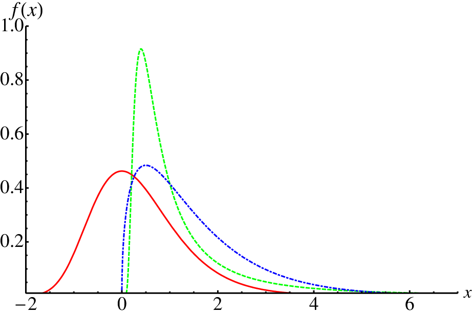
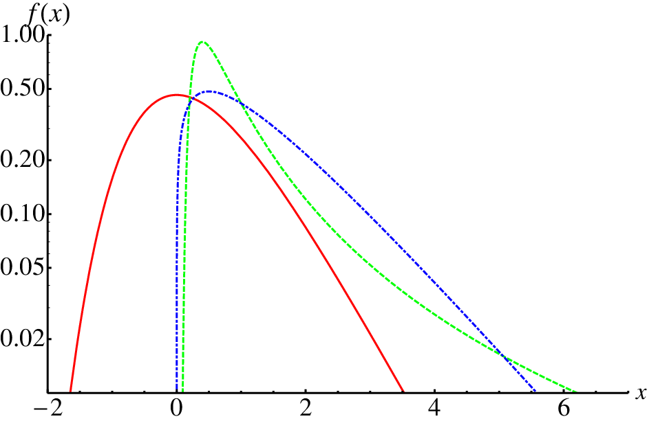
As a rather generic illustration, let us consider the case when the potentials and are given by
| (20) |
with , . If , the particles and the piston are in a constant external force field, like the (local) gravity field, in which case and . If , the piston is for instance linked to the hard wall situated at with a spring of stiffness .
In order to determine the limit distribution of the volume fluctuations in the large limit, the parameter characterizing the small behaviour of should be evaluated. Considering Eq. (15), one needs to compute first the function in the small limit, which is deduced from the large limit of . Given that
| (21) |
with the Euler Gamma function, one has in the large limit
| (22) |
Inverting the relation to get , one finds to leading order in the limit
| (23) |
We now wish to compute . Putting Eq. (23) into Eq. (15), one needs to distinguish between the cases and .
If , one gets
| (24) |
with . Therefore, behaves as a power law in the small limit, up to logarithmic corrections which do not modify the asymptotic distribution (see Appendix B). It follows that volume fluctuations are described by a Gumbel distribution with parameter [19], which compares the relative intensity of the compression force acting on the piston and of the forces directly acting on the particles. In the limit of a strong compression force , volume fluctuations asymptotically become Gaussian, as the generalized Gumbel distribution converges to the normal distribution in this limit. In the opposit limit where the external compression force is small with respect to the forces acting on the particles, the generalized Gumbel distribution converges to an exponential distribution (see Appendix A).
In the case where the confining potential for the gas and that for the piston are of different functional form, , one finds for , dropping logarithmic corrections as well as constants of order unity,
| (25) |
Hence does not behave as a power law when , so that the results of [19] do not apply. We show in Appendix C that when , the limit distribution is a Gaussian law, while for the limit distribution is exponential. This result is consistent with the following intuitive argument. When , decays faster than any power law, and one expects this situation to be similar to the large limit, for which a Gaussian distribution is recovered. In contrast, when , decays slower than any power law, which is expected to be similar to the limit , in which case one obtains an exponential distribution, as shown in Appendix A. The physical interpretation is that for the piston confines the gas more strongly that the bulk confining potential, so that the latter becomes irrelevant at large size, leading to a regular confined gas with standard thermodynamic properties. For the reverse is true; the gas is confined by the bulk potential; the piston becomes irrelevant and its fluctuations become those of a piece of flotsam driven by the fluctuations of the confined gas below.
Note that we focused here on power law potentials, which correspond to a quite natural class of potentials. However, one could also consider logarithmic potentials and , which would lead to Fréchet distributions given in Eq. (18) for the volume fluctuations. Alternatively, if the potential diverges for a finite value , (for instance by adding a rigid wall on top of the piston), the asymptotic distribution of fluctuations would be of the Weibull type, as described in Eq. (19).
4 Discussion: relation with thermodynamics
In the present paper, we have shown that the volume fluctuations of an ideal gas of classical and independent particles confined by an algebraic potential acting on both particles and piston along one dimension and by hard walls in the perpendicular directions, are described by generalized extreme value statistics. In the simple case when the piston is identical to the particles, the appearance of standard extreme value distributions is easily understood from a direct mapping of volume fluctuations onto an extreme value problem of independent and identically distributed (i.i.d.) random variables.
In a more general situation the piston can differ from the particles in two ways; either the confining potential is of the same form but of different amplitude, meaning that the restoring forces on the particle and piston are different. Or, the functional form is different. In the first situation non-Gaussian height fluctuations still occur in the limit of large in the form of generalized extreme value distributions parameterized by a real variable, . If the restoring force on the piston becomes much larger than that on the particles, the distribution crosses over to Gaussian. Yet for fixed values of the forces, that is for fixed , the distributions are non-Gaussian for all system sizes and no crossover occurs as a function of . For different functional forms, a crossover does occur as a function of system size, either to Gaussian fluctuations if the piston is strongly confined, or to one-body non-Gaussian statistics, with exponential height fluctuations if the piston is less strongly confined. Our results are, in principle valid for a system of arbitrary scale perpendicular to the axis. However, non-Gaussian fluctuations should be observable for of order unity only, which implies a piston of microscopic extent perpendicular to , ensuring that any experimental realization would be in the form of a quasi-one dimensional sample (another possibility could be to exert two different forces on the piston, that could be fine-tuned to compensate almost exactly).
Non-Gaussian volume fluctuations have strong consequences for the thermodynamics. In previous work, non-Gaussian order parameter fluctuations have been related to critical phenomena or to the fact that an ordered phase is unstable in low dimensions [11, 28]. Analogous physics occurs for the models considered here: non-Gaussian volume fluctuations lead to singular thermodynamics. To illustrate this we consider first the simplest case where piston and particles are identical, of mass and confined by a gravitational force, , so that . In this case the height difference variables defined in (8), are independent and exponentially distributed:
| (26) |
as seen from Eq. (9). One then has a -noise-like spectrum [3], , giving directly
| (27) |
where is the characteristic length scale for the particles set by the gravitational field. Defining volume and external pressure, , leads to an equation of state for the confined ideal gas in the large limit. This singular non-extensive behavior signifies the crossover between a system confined by a bulk potential (the gravitational field on the particles) and an external constraint (the pressure imposed by the piston). It is mathematically equivalent to the case of a thermally excited one dimensional interface with long range interactions [3].
Let us now consider the case where the piston mass is different from the mass of the particles. In this case, the variables are still exponentially distributed, but now with
| (28) |
similarly to the “truncated -noise” considered in [18, 19]. The average piston position is then given by
| (29) |
For large , one can approximate the sum by an integral, yielding
| (30) |
Introducing again the (external) pressure , one finds the equation of state
| (31) |
where now is a function of pressure. Hence, again we find that non-Gaussian fluctuations are associated with non-extensive thermodynamics. The ratio compares the total mass of the particles to the mass of the piston (the mass could also be an effective mass accounting for the constant force , positive or negative, exerted by an operator: ). If the piston becomes macroscopic with total mass, , exceeding that of the gas, then we move into the regime where . In this regime, we recover the ideal gas equation of state, , as well as Gaussian volume fluctuations. In the opposite case where (typically if is finite and is large), one has non-Gaussian fluctuations as described in Sect. 4, and the non-extensive equation of state . Assuming that is large but finite, and scaling the number of particles, , with all other parameters held fixed, one therefore begins in the extensive regime for small (but macroscopic) and . In this regime is less than and the effect of the confining field on the particles is negligible. On increasing , one crosses over into the non-extensive regime when this length scale in exceeded. However, no crossover is observed in the statistics of fluctuations since is large, and fluctuations are practically Gaussian even in the non-extensive regime. Taking requires more calculation but leads to essentially equivalent results.
A consequence of these results is that in the non-extensive regime the volume fluctuations are abnormally small on the scale set by the mean volume or the number of particles. Through the fluctuation dissipation relation, this scale is given by
| (32) |
which, in the limit is independent of . Hence the isothermal compressibility, , a normally intensive measure of the fluctuations, varies as and scales to zero in the limit, . Physically this result occurs because the potential confining the particles within the bulk of the sample suppresses the collective fluctuations present in the standard thermodynamic regime. The logarithmic dependence is characteristic of a marginal situation between the two regimes and is analogue to the marginal stability of an ordered phase at the lower critical dimension, such as the 2D-XY model [11], or one dimensional interface with long range interactions [3].
The case where the piston is more confined than the particles is best illustrated by removing the confining potential for the particles in the above example while keeping that for the piston. One now trivially finds the ideal gas equation of state, and regular thermodynamic fluctuations from Eq. (3).
Appendix A Large and small limits of the generalized Gumbel distribution
In this appendix, we wish to show that the generalized Gumbel distribution converges to the Gaussian distribution when , and to the exponential distribution when . The distribution is defined in Eq. (17), with , and given by [19]
| (33) |
The function is the digamma function defined as
| (34) |
where is the Euler Gamma function.
Let us start with the case , and determine the large behaviour of the constants and given in (33). Using Stirling’s approximation for the Gamma function,
| (35) |
one finds
| (36) | |||||
| (37) |
so that and are given for large by
| (38) |
It follows that
| (39) |
Hence for fixed , goes to zero when , so that the term can be expanded to second order. Inserting the different asymptotic expansion given above in the generalized Gumbel distribution leads to, up to order corrections in the exponential,
| (40) |
yielding in the infinite limit the standard Gaussian distribution
| (41) |
In the opposite limit , the Gamma function behaves as , so that and
| (42) |
The normalization factor reads
| (43) |
Using , one finds for
| (44) | |||||
| (45) |
It is easily seen that the second factor in the r.h.s. converges to a Heaviside function for ,
| (46) |
so that the generalized Gumbel distribution converges to the exponential distribution with zero mean and unit variance
| (47) |
Appendix B Case : Effect of logarithmic corrections
The aim of this appendix is to show that the logarithmic corrections appearing in Eq. (24) do not change the asymptotic distribution. To that purpose, we follow closely the procedure of [19], and keep essentially the same notations. Using Eq. (10) and the results of [19], the distribution is given by
| (48) |
We assume for a power-law form with logarithmic corrections when , namely
| (49) |
Let us define the value such that . In the limit , diverges as when . Introducing the auxiliary function , we perform the following change of variables, to look at fluctuations around :
| (50) |
Expanding in the neighbourhood of leads to
| (51) |
where
| (52) |
The distribution is obtained from as
| (53) | |||||
where we have used . In the large limit, we have, keeping fixed,
| (54) | |||
| (55) | |||
| (56) |
Using Eq. (49), one obtains for large , as ,
| (57) | |||||
| (58) |
Altogether, one finds
| (59) |
Let us now compute , which is given by [19]
| (60) |
With the change of variable , we get for large
| (61) |
Using the small expansion of , one has
| (62) | |||||
Coming back to the distribution , one finally obtains from Eq. (59)
| (63) |
which is precisely the generalized Gumbel distribution. In order to recover the standard expression given in Eq. (17), one simply needs to introduce the normalized variable through , with and defined in Eq. (33).
Appendix C Case : Convergence of the volume distribution toward Gaussian and exponential laws
In this appendix, we compute the asymptotic volume distribution in the case where is given by
| (64) |
with , (we refer to Sect. 3 for notations), and . The derivation follows essentially the same steps as in Appendix B, but also bears some similarities with that done in Appendix A. The distribution is given by
| (65) |
Using the form (64) of and recalling that , one finds for large
| (66) |
We now make the following change of variables:
| (67) |
where is defined by . One then has for large
| (68) |
The distribution reads
| (69) |
In the case , when , so that
| (70) |
and converges to the exponential distribution (the prefactor converges to by normalization of the distribution).
In the opposite case , the above argument does not apply anymore. Thus we start again from Eq. (69), and make a saddle point calculation. Let us introduce the function such that , namely
| (71) |
with
| (72) |
We define through , leading to
| (73) |
We then perform a change of variable
| (74) |
For large , we expand the term appearing in to second order, yielding
| (75) |
The resulting distribution of ,
| (76) |
then converges to a Gaussian law when (here again, the normalization of the distribution ensures that the prefactor converges to the correct limit).
References
References
- [1] E. J. Gumbel, Statistics of Extremes (Columbia University Press, 1958; Dover publication, 2004).
- [2] J. Galambos, The asymptotic theory of extreme order statistics (Wiley & Sons, 1987).
- [3] T. Antal, M. Droz, G. Györgyi and Z. Rácz, Phys. Rev. Lett. 87, 240601 (2001); Phys. Rev. E 65, 046140 (2002).
- [4] G. Györgyi, P. C. W. Holdsworth, B. Portelli and Z. Rácz, Phys. Rev. E 68, 056116 (2003).
- [5] A. A. Fedorenko and S. Stepanow, Phys. Rev. E 68, 056115 (2003).
- [6] F. van Wijland, Physica A 332, 360 (2004).
- [7] A. Comtet, P. Leboeuf, S. N. Majumdar, Phys. Rev. Lett. 98, 070404 (2007).
- [8] A. Comtet, S. N. Majumdar, S. Ouvry, J. Phys. A 40, 11255 (2007).
- [9] S. T. Bramwell, P. C. W. Holdsworth, and J.-F. Pinton, Nature (London) 396, 552 (1998).
- [10] S. T. Bramwell et. al., Phys. Rev. Lett. 84, 3744 (2000);
- [11] S. T. Bramwell et. al., Phys. Rev. E 63, 041106 (2001).
- [12] B. Portelli, P. C. W. Holdsworth, M. Sellito, and S. T. Bramwell, Phys. Rev. E 64, 036111 (2001).
- [13] A. Noullez and J.-F. Pinton, Eur. Phys. J. B28, 231 (2002).
- [14] C. Chamon, P. Charbonneau, L. F. Cugliandolo, D. R. Reichman, and M. Sellitto, J. Chem. Phys. 121, 10120 (2004).
- [15] L. D. C. Jaubert, C. Chamon, L. F. Cugliandolo, M. Picco, J. Stat. Mech. P05001 (2007).
- [16] J. J. Brey, M. I. Garcia de Soria, P. Maynar and M. J. Ruiz-Montero, Phys. Rev. Lett. 94, 098001 (2005).
- [17] S. Joubaud, A. Petrosyan, S. Ciliberto, and N. B. Garnier, Phys. Rev. Lett. 100, 180601 (2008).
- [18] E. Bertin, Phys. Rev. Lett. 95, 170601 (2005).
- [19] E. Bertin and M. Clusel, J. Phys. A 39, 7607 (2006).
- [20] H. L. Frisch, Phys. Rev. 104, 1 (1956).
- [21] D. W. Jepsen, J. Math. Phys. 6, 405 (1965).
- [22] J. L. Lebowitz and J. K. Percus, Phys. Rev. 155, 122 (1967).
- [23] J. Piasecki, J. Stat. Phys. 104, 1145 (2001).
- [24] V. Balakrishnan, I. Bena, and C. Van den Broeck, Phys. Rev. E 65, 031102 (2002).
- [25] I. Bena and S. N. Majumdar, Phys. Rev. E 75, 051103 (2007).
- [26] See, e.g., V. V. Petrov, Sums of independent random variables, Springer-Verlag (1975).
- [27] See, e.g., G. H. Wannier, Statistical Physics (Wiley, New York, 1966).
- [28] N. D. Mermin and H. Wagner, Phys. Rev. Lett. 17, 1133 (1966).