Detecting gravitational wave emission from the known accreting neutron stars

Anna L. Watts Affiliation: Max Planck Institut für Astrophysik, Karl-Schwarzschild-Strasse 1, 85741 Garching, Germany Affiliation: Astronomical Institute “Anton Pannekoek”, Kruislaan 403, 1098 SJ Amsterdam, The Netherlands; A.L.Watts@uva.nl Badri Krishnan Affiliation: Albert-Einstein-Institut, Max-Planck-Institut für Gravitationsphysik, Am Mühlenberg 1, 14476 Golm, Germany Lars Bildsten Affiliation: Kavli Institute for Theoretical Physics, Kohn Hall, University of California at Santa Barbara, CA 93106, USA Bernard F. Schutz Affiliation: Albert-Einstein-Institut, Max-Planck-Institut für Gravitationsphysik, Am Mühlenberg 1, 14476 Golm, Germany

Abstract

Detection of gravitational waves from accreting neutron stars (NSs) in our galaxy, due to ellipticity or internal oscillation, would be a breakthrough in our understanding of compact objects and explain the absence of NSs rotating near the break-up limit. Direct detection, however, poses a formidable challenge. Using the current data available on the properties of the accreting NSs in Low Mass X-Ray Binaries (LMXBs), we quantify the detectability for the known accreting NSs, considering various emission scenarios and taking into account the negative impact of parameter uncertainty on the data analysis process. Only a few of the persistently bright NSs accreting at rates near the Eddington limit are detectable by Advanced LIGO if they are emitting gravitational waves at a rate matching the torque from accretion. A larger fraction of the known population is detectable if the spin and orbital parameters are known in advance, especially with the narrow-band Advanced LIGO. We identify the most promising targets, and list specific actions that would lead to significant improvements in detection probability. These include astronomical observations (especially for unknown orbital periods), improvements in data analysis algorithms and capabilities, and further detector development.

Keywords:

accretion, accretion disks—gravitational waves—stars: neutron—stars: rotation—X-rays: binaries—X-rays: bursts

1 Introduction

A number of interferometric gravitational wave observatories have been built with the intention of opening a new observational window for studying astrophysical objects. These include the LIGO¹¹ 1 http://www.ligo.caltech.edu, GEO²² 2 http://geo600.aei.mpg.de/, VIRGO³³ 3 http://wwwcascina.virgo.infn.it and TAMA⁴⁴ 4 http://tamago.mtk.nao.ac.jp detectors. The TAMA and LIGO Scientific Collaborations have demonstrated their ability to reach sensitivity goals, take year-long stretches of data with good duty cycles, and analyse the data to set, with confidence, upper limits on the emission from a number of possible sources. At present the large LIGO and VIRGO detectors are performing a significant sensitivity upgrade. This is therefore a good time to carry out a realistic study of the challenges of searching for gravitational waves from one class of sources that future upgrades may render detectable: spinning neutron stars (NSs) in Low Mass X-ray Binaries (LMXBs).

For the last ten years, ever since a paper by one of us (Bildsten, 1998) suggested that LMXBs could be steady beacons of gravitational waves, the study of LMXBs (and especially of the source Scorpius X-1) has been one of the scientific goals of the development of detectors with greatly improved sensitivity. Since then, X-ray astronomers have gathered a wealth of new data on these sources, astrophysicists have built better models, and gravitational wave scientists have gained considerable experience of their ability to extract weak signals from data streams. It is timely, therefore, to revisit these estimates.

The expectation that LMXBs could be strong steady sources of gravitational waves originates in one of the most important outstanding questions about NSs: why they all spin at frequencies much less than the break-up limit of 1 kHz (Lattimer & Prakash, 2007). Simple estimates (Cook, Shapiro & Teukolsky, 1994) of the spin-up timescales for accreting NSs in LMXBs suggest that there should be no difficulty in reaching at least 1 kHz. The fastest rotating accreting pulsar is at 599 Hz (Galloway et al., 2005) and many NS rotate much more slowly (Chakrabarty et al., 2003). The millisecond radio pulsars, the likely offspring of LMXBs, also spin at slower rates than expected. The current record stands at 716 Hz (Hessels et al., 2006) and surveys in nearby globular clusters continue to reveal a paucity of rapid rotators (Ransom et al., 2005; Hessels et al., 2007; Freire et al., 2008). Whether the apparent spin limit is genuine remains to be resolved. Nevertheless, given the current sample, it certainly appears that there is some brake that prevents accreting NSs from reaching the break-up limit.

The candidate mechanisms fall into two main camps. In the first, accretion torques are reduced and eventually balanced by the interaction between the accretion disk and the NS’s magnetic field (Ghosh & Lamb, 1978; White & Zhang, 1997; Andersson et al., 2005). The second possibility, and our focus here, is the loss of angular momentum via the emission of gravitational radiation (Papaloizou & Pringle, 1978; Wagoner, 1984; Bildsten, 1998). There are many conceivable ways for an accreting NS to develop a quadrupolar asymmetry that leads to gravitational wave (GW) emission: crustal mountains (Bildsten, 1998; Ushomirsky, Cutler & Bildsten, 2000; Melatos & Payne, 2005; Payne & Melatos, 2006; Haskell, Jones & Andersson, 2006), magnetic deformation (Cutler, 2002; Haskell et al., 2008) or internal r-mode oscillations (Bildsten, 1998; Andersson, Kokkotas & Stergioulas, 1999; Levin, 1999; Andersson et al., 2000; Heyl, 2002; Andersson, Jones & Kokkotas, 2002; Wagoner, 2002; Nayyar & Owen, 2006; Bondarescu, Teukolsky & Wasserman, 2007). The exciting prediction from all GW emission scenarios is the possible direct detection of an accreting NS by a ground-based interferometric gravitational wave detector.

Searches for periodic GWs from NSs have already been performed with the LIGO and GEO detectors. These include searches of known radio pulsars (Abbott et al., 2004; Abbott et al., 2005b; Abbott et al., 2007b), assuming the phase of the GW signal to be locked to the known NS rotation, and wide parameter surveys for hitherto unknown NSs (Abbott et al., 2005a; Abbott et al., 2007a; Abbott et al., 2008). There have also been searches for GWs from the accreting NS Scorpius X-1. The first (Abbott et al., 2007a) used a coherent statistic on a template grid utilising 6 hours of data (limited by computational requirements) from the second science run of the two LIGO 4 km interferometers, followed by a coincidence analysis between candidates from the two detectors. The second search (Abbott et al., 2007c) used a method of cross-correlating the outputs of the two LIGO 4 km detectors using about 20 days of coincident data taken during the fourth science run. Data from resonant bar detectors have also been used in these searches; see e.g. Astone et al. (2002); Astone et al. (2005) for a blind all-sky search in a narrow frequency band using data from the EXPLORER detector.

These early searches, while so far yielding only upper limits, have served to develop and prove data analysis methods that will be used on data from future, more sensitive searches. The VIRGO detector is approaching its design sensitivity and the LIGO detectors have just completed a full run at their first-stage design sensitivity. An initial upgrade of LIGO is about to commence, followed by a full upgrade to Advanced LIGO⁵⁵ 5 http://www.ligo.caltech.edu/advLIGO in the next decade. VIRGO expects to parallel these developments. These impending improvements in GW sensitivity, coupled with the experience of performing realistic data analysis, make the time right to assess what the relevant accreting NS properties tell us about the ultimate detectability of NS sources.

This paper explains the prospects for detecting GWs from accreting NSs, and identifies the most promising targets. We start in Section 2 with the best case scenario, highlighting the data analysis challenges and the need for detailed information on the accreting NS properties, which are presented in Section 3. Section 4 explains fully the GW search data analysis challenges and the direct consequences of parameter uncertainty on integration times and detection statistics, allowing us to assess future detectability in Section 5. We close in Section 6 by highlighting where progress can be made in the short-term on NS source properties, and the implications for current and future gravitational wave searches.

2 Overview and Best Case Estimates

The potential strength of a periodic GW signal at frequency $\nu$ from specific LMXBs with accretion rates $\dot{M}$ was estimated by Bildsten (1998) (hereafter B98) in the mountain scenario. In this model a quadrupole moment $Q$ , that is stationary in the rotating frame of the star (a ‘mountain’), leads to the emission of gravitational waves with a predominant frequency $\nu=2\nu_{s}$ , $\nu_{s}$ being the spin frequency of the NS. The assumption is that the accretion torque on a NS of mass $M$ and radius $R$

N_{a}=\dot{M}\left(GMR\right)^{1/2},

(1)

is balanced by the GW torque

N_{\rm gw}=-\frac{32GQ^{2}\Omega_{s}^{5}}{5c^{5}},

(2)

where $\Omega_{s}=2\pi\nu_{s}$ is the angular frequency of the star. The accretion rate is estimated from the bolometric X-ray flux $F$ by assuming that the luminosity is $L\approx GM\dot{M}/R$ , yielding

\dot{M}=\frac{4\pi Rd^{2}F}{GM},

(3)

where $d$ is the distance to the source. The predicted gravitational wave amplitude $h_{0}$ (as defined in Jaranowski, Królak & Schutz (1998))⁶⁶ 6 Note that flux formulae are often given in terms of an angular and time-averaged amplitude $h$ rather than in terms of $h_{0}$ . In Owen et al. (1998) and Andersson, Kokkotas & Stergioulas (1999), for example, the quoted amplitude $h^{2}=2h_{0}^{2}/5$ . can be written in terms of the GW luminosity, $\dot{E}_{\rm gw}=N_{\rm gw}\Omega_{s}$ , as

h_{0}^{2}=\frac{5G}{2\pi^{2}c^{3}d^{2}\nu^{2}}\dot{E}_{\rm gw}.

(4)

Under the condition of torque balance,

h_{0}=3\times 10^{-27}F_{-8}^{1/2}\left({R\over{\rm 10km}}\right)^{3/4}\left({1.4M_{\odot}\over M}\right)^{1/4}\left(\frac{{\rm 1~kHz}}{\nu_{s}}\right)^{1/2},

(5)

where $F_{-8}=F/10^{-8}{\rm erg\ cm^{-2}\ s^{-1}}$ . Equation (5) makes it clear that the GW signal strength depends on two observables, the flux on the sky from the LMXB and the NS spin rate (Wagoner, 1984; Bildsten, 1998). This amplitude is then compared directly to the best case detectable amplitude in a long search, $h_{0}^{\rm sens}$ , which we will derive shortly.

These amplitudes are sufficiently weak that long stretches of data must be folded, using predicted signal templates. This is called matched filtering, and its sensitivity improves with the square-root of the observation time, provided that the template manages to keep phase with the real signal to within about one radian over the entire duration. Where spin and orbital parameters are poorly constrained, many templates must therefore be searched. Analysis can become statistically and computationally untenable, and computational loads may limit integration times and thereby detectability. Contrast for example the most recent searches for radio pulsars, where a precise timing ephemeris is available (Abbott et al., 2007b), with searches for the closest accreting neutron star Scorpius X-1 (Abbott et al., 2007c). Poor constraints on the spin and orbital parameters for Sco X-1 necessitate multiple templates. This reduces the feasible integration time substantially, resulting in upper limits that are approximately two orders of magnitude larger than those obtained for the best radio pulsar. We begin our discussion there.

2.1 Spin Frequencies of Accreting NSs

The discoveries and studies with the Rossi X-ray Timing Explorer (RXTE) over the last ten years have dramatically improved our understanding of stellar spin rate, $\nu_{s}$ (Strohmayer & Bildsten, 2006; van der Klis, 2006). Having some constraint on the spin is, as will become clear in later Sections, the most important factor determining the feasibility of gravitational wave searches. For this reason we concentrate only on sources for which there is some measurement or estimate of $\nu_{s}$ . We now summarize the three relevant categories of accreting NSs: accreting millisecond pulsars, burst oscillation sources, and kiloHertz Quasi-Periodic Oscillation (kHz QPO) sources.

The spin is measured directly in the accreting millisecond pulsars, where fixed hotspots, presumably at the magnetic footpoints, are a permanent asymmetry. In 1998 only one such object was known; there are now ten members of this class, three of which show only intermittent pulsations. The other measures of spin are indirect. Probably the most reliable are burst oscillations, seen during Type I X-ray bursts (when accreted material burns in an unstable thermonuclear flash). In 1998 there were six burst oscillation sources: there are now twelve stars with burst oscillations seen in multiple bursts (including three pulsars), and seven stars with tentative detections.

For the three accreting millisecond pulsars that also show burst oscillations, the burst oscillation frequency is at or very close to the known spin frequency (Chakrabarty et al., 2003; Strohmayer et al., 2003; Altamirano et al., 2008). It would therefore seem reasonable to equate the burst oscillation frequency with the spin frequency for the non-pulsing sources (as was done in B98). The frequency for a given source is highly consistent from burst to burst, implying that there is at least a strong dependence on stellar spin (Strohmayer et al., 1998a; Muno, Özel & Chakrabarty, 2002). The detection of highly coherent oscillations lasting several hundred seconds during a superburst adds further support to this hypothesis (Strohmayer & Markwardt, 2002). There are, however, some complicating factors. Firstly, burst oscillations can exhibit frequency drifts of up to a few Hz. Secondly, there are some differences in the properties of the burst oscillations of the non-pulsing LMXBs as compared to the pulsars (see for example Watts & Strohmayer (2006)), suggesting that the mechanism may differ. In models that involve global modes of the surface layers, for example, the observed frequency would be offset from spin frequency by several Hz (Heyl, 2004; Piro & Bildsten, 2005).

The third class of sources to be considered are those which exhibit twin kHz QPOs. Early observations suggested that although the frequencies could shift, their separation remained relatively constant, implying a link to stellar spin. We now know that separation varies (often quite substantially) as accretion rate changes, and the cause of the kHz QPOs is still not understood. However, most models still depend in some way on the stellar spin, either directly or via the influence on the space-time in the inner regions of the accretion disk (see van der Klis (2006) for a recent and comprehensive review). Observations of twin kHz QPOs in two of the accreting millisecond pulsars have done little to resolve the situation: in one case separation is rather close to the spin frequency; in the other it is slightly less than half the spin (Wijnands et al., 2003a; Linares et al., 2005). Whether there is any link between kHz QPO separation and stellar spin will doubtless emerge in due course. However, given that most models still predict some relation, we follow B98 and include these stars in our analysis.

2.2 Optimal Gravitational Wave Detection

Before being scaled down for their current sensitivity upgrades, the first generation LIGO interferometers operated for nearly two years at or better than their design sensitivity, by the end of which the first generation Virgo detector was not far behind. The “Enhanced” LIGO and VIRGO interferometers should begin operation in 2009, and the Advanced LIGO interferometers are now funded and should be operational by 2014. Advanced VIRGO is expected on the same schedule. Beyond this, there are ambitious plans for a third generation Einstein Telescope (ET) in Europe.

The sensitivity of a gravitational wave detector is determined by the power spectral density of its instrumental strain noise, normalized to an equivalent gravitational-wave amplitude $h(t)$ . This is just the Fourier power spectrum of $h(t)$ and is called $S_{h}(\nu)$ : the noise power per unit frequency. It is conventional to plot $h(\nu)=[S_{h}(\nu)]^{1/2}$ , which allows comparison of the noise to the signal’s amplitude if one knows the signal’s bandwidth. The sensitivity curves of current and future detectors are shown in Figure 1. The design noise curves for Initial LIGO, Virgo and ET are taken from analytic models available, for example, in the LIGO software repository⁷⁷ 7 http://www.lsc-group.phys.uwm.edu/daswg/projects/lal.html. The most recent science runs of the LIGO detectors have in fact reached their design goals over a broad frequency range of interest, above $\sim 40$ Hz. The Enhanced LIGO noise curve in Figure 1 is a realistic estimate of what can be achieved; thus at low frequencies (below $\sim$ 40 Hz), the Enhanced LIGO noise curve lies above the Initial LIGO design curve.

The Advanced LIGO detector configurations have not yet been finalized, and we therefore need to consider different possibilities. Advanced LIGO can potentially be operated in a narrow band mode where sensitivity is gained in a relatively narrow frequency range at the expense of broad band sensitivity (see e.g. Meers (1988); Buonanno & Chen (2002)). This could be particularly relevant for periodic signals where the frequency is well known. The first panel of Figure 1 shows an example of such a narrow band noise curve⁸⁸ 8 The various Advanced LIGO noise curves shown here have been obtained using version 6.2 of the Matlab script “Bench”. It is worth mentioning that a newer version of Bench, v7.0, is currently under development which includes an improvement in coating thermal noise; it is probably worth re-calculating the Advanced LIGO noise curves once this and later versions become available. The noise curve can be tuned to target a broad range of frequencies by changing a number of interferometer parameters, and for our purposes, the value of the noise at the minimum is especially important. Thus, the lower panel of Fig. 1 shows the lower envelope of the narrow band noise curves above 100 Hz. Between 100 Hz and about 400 Hz, the narrow band curves are limited by thermal noise, and by quantum noise at higher frequencies⁹⁹ 9 To generate the lower envelope of the narrow band noise curves, we have used Bench to calculate the narrow band noise curves for a range of choices for a few interferometer parameters. These parameters are the phase and transmittance of the signal recycling cavity, and the transmittance the input test mirror and the power recycling mirror. The envelope is then obtained by calculating the convex hull of the minima of the various noise curves.. See Section 6.4 for additional discussion. It is important to keep in mind that the narrow-band “envelope” does not represent any particular interferometer configuration but is rather a superposition of many configurations. It is only useful for targeting narrow-band signals with frequency uncertainties of, say, $\mathcal{O}(10)\,$ Hz in which case we can choose the appropriate element from the set of configurations used to produce the envelope. Finally, note that possible designs for the third generation detectors are still being explored, and thus the noise curve for the Einstein Telescope is much more preliminary.

Refer to caption — Figure 1: The noise curves for Initial LIGO, Virgo, Advanced LIGO, and the third generation Einstein Telescope (ET) interferometers. The Initial, Enhanced and Advanced LIGO curves are labelled “I-LIGO”, “E-LIGO” and “A-LIGO” respectively; “ET” is Einstein Telescope. There are three curves for Advanced LIGO in each panel. The top panel shows a nominal broad band configuration (the so called “zero de-tuned” configuration), an example of a narrow band curve (“A-LIGO NB EX”), and the total thermal noise (“A-LIGO TH”), i.e. the sum of the suspension and mirror thermal noise curves. The lower panel shows the lower envelope of the narrow band curves (“A-LIGO NB ENV”) instead of the narrow band example. The thermal noise is shown because it is sometimes taken as a theoretical lower bound on the narrow banding for frequencies above, say, 100 Hz; as seen from the lower panel, this is not a good approximation at higher frequencies.

To start addressing the question of detecting GWs from LMXBs, we start by asking how strong the signal would need to be for detection if we knew all source parameters to sufficient accuracy that only one template was needed (a coherent fold). Computational cost is no issue, and we can easily integrate for long periods $T_{\rm obs}$ . Such a fully coherent search with $D$ detectors of comparable sensitivity is a best case and defines a signal-to-noise ratio (SNR) as ${\rm SNR}^{2}=h_{0}^{2}T_{\rm obs}D/S_{n}$ ; thus, the SNR-squared builds up linearly with the observation time (here $S_{n}(\nu)$ is the power-spectral density of the detector noise). Conversely, for a given choice of SNR threshold for detectability, this leads to a minimum detectable signal amplitude $h_{0}$ (following the notation of Jaranowski, Królak & Schutz (1998)):

h_{0}\approx 11.4\sqrt{\frac{S_{n}}{DT_{\rm obs}}}\,

(6)

which is a useful indicator of the sensitivity of such a search. The factor of 11.4 corresponds to an SNR threshold which would lead to a single trial false alarm rate of $1\%$ and a false dismissal rate of $10\%$ (Abbott et al., 2007a) and a uniform averaging over all possible source orientations and sky positons (Jaranowski, Królak & Schutz, 1998).

Figure 2 compares the predicted and detectable amplitudes for this best-case scenario using the long-term flux average derived in Section 3 and summarised in Table 1, and assuming that each NS is in perfect spin balance (so that we can neglect spin derivatives), with gravitational wave torque balancing that of accretion. We assume that the spin frequency for the kHz QPO sources lies in the middle of the known range of separations, and take $T_{\rm obs}=2\,$ years as a reference value.

Figure 2 naively implies that the kHz sources are the most easily detected sources. However, they offer a specific challenge, as we do not know many of their spins or orbital parameters. Detecting the GW signal requires a knowledge of the GW phase evolution which depends crucially on the orbital parameters. Ignorance or inaccurate knowledge of the orbit could then require a search over a significant number of parameters and as we shall see, this can have a dramatic impact on the sensitivity of the GW search. Hence assessing the detectability of GWs requires a more careful description of the mechanics of the gravitational wave data analysis process. Most of this paper is therefore focused on clearly assessing the data analysis challenges for present and future generations of GW detectors that takes into account the limitations imposed by incomplete astrophysical knowledge and finite computational resources.

3 Accreting Neutron Star Properties

In this Section we summarize our knowledge of the relevant search parameters for all accreting NSs in LMXBs where there is some estimate of the spin: the accreting millisecond pulsars, the burst oscillation sources, and the kHz QPO sources. This sample contains both atoll and Z sources, a classification determined by the spectral and timing properties (Hasinger & van der Klis, 1989; Muno, Remillard & Chakrabarty, 2002; Gierliński & Done, 2002; van der Klis, 2006). As explained in Section 2 we require flux histories, spin frequencies and orbital parameters, some of which are measured, whilst others can only be estimated. We also need to gauge the uncertainty on each quantity. This sets the required search parameter space, and in Section 5 we use this information to compute the number of signal templates required for each source.

This Section is rather lengthy, as we give full details of the provenance of all of the values used in our study. There are two main reasons for this: firstly, to make clear the link between the astronomical observations and the consequences for gravitational wave searches. Secondly, many of the values that we derive involve assumptions, or draw on old or uncertain measurements: where this is the case we wanted to make it explicit, in order to drive future astrophysical modelling and observations. The information in this Section should also be a useful resource for anyone intending to carry out a search for gravitational waves from these objects, or for future detectability studies. Readers who are not concerned with the details of the source properties and uncertainties can however skip this Section, and will find the key results summarized in Tables 1 - 4.

3.1 Constraining Fluxes and Accretion Rates

The observed flux, $F$ , sets the expected GW signal strength (Equation 5). For persistent sources we record only the long-term average flux, $F_{\rm av}$ , whereas for transient sources we also record the outburst flux, $F_{\rm ob}$ (averaged over outbursts and quiescent periods). Bolometric outburst fluences have been computed for the accreting millisecond pulsars, but for the majority of sources this is not the case. For the remaining sources we determine $F$ using data from the RXTE All Sky Monitor (ASM), which provides a near-continuous history of source activity from 1996 to the present in the 2-10 keV band (Levine et al., 1996). Converting the 2-10 keV flux to a bolometric flux requires detailed spectral modelling. For most burst oscillation sources we use the results of Galloway et al. (2008): these authors carry out spectral modelling using the pointed RXTE PCA data (2.5-25 keV) to estimate bolometric flux. We compare the calculated fluxes to the ASM countrate at the time of the observation to establish this relationship. For the transient sources we only include in our integrated ASM histories the times when the source is in outburst and detectable above a $3\sigma$ level. This avoids contamination from other sources in the field which would overestimate the long-term flux. This method of estimating flux history introduces some errors, since spectral shapes (and the correction from 2-10 keV flux to bolometric flux) will change: but it gives a reasonable estimate. This uncertainty should however be borne in mind in Section 6 for those sources that are on the margins of detectability.

We also record position and distance. Source position must be known to a certain degree of precision for the long folds that this type of analysis necessitates (Section 4.1). We have listed the most accurate and up to date position known for the X-ray source or its optical, infra-red or radio counterpart. Source distance, which is relevant for the emission modelling in Section 5, can be estimated in several different ways. Only for the closest source in our sample, Sco X-1, can the distance be measured via parallax. For the other sources different methods are used: location of the source in a globular cluster; the presence of radius expansion X-ray bursts (where luminosity reaches the Eddington limit¹⁰¹⁰ 10 The Eddington limit depends on the composition. Sometimes composition can be inferred from burst properties, but this is not always the case, leading to additional uncertainty. See also Galloway, Özel & Psaltis (2008).); inferences about mass transfer from the long-term X-ray flux, assuming that the binary orbit evolves due to gravitational wave emission; absorption and spectral modelling.

We give details of pulsar frequency, burst oscillation frequency, and twin kHz QPO separation, as measured with RXTE’s Proportional Counter Array (PCA). For sources with only a burst oscillation frequency, we assume that $\nu_{s}$ lies within $\pm 5$ Hz of the burst oscillation frequency $\nu_{b}$ . For the kHz QPO sources we assume that the spin lies within the reported range of kHz QPO separations. We review both of these assumptions in more detail in later Sections.

3.2 Orbital Uncertainties

We must know (or presume) the orbital parameters in order to fold long stretches of gravitational wave data, most importantly, the orbital period $P_{\rm orb}$ and eccentricity, $e$ . We also need a reference time within the orbit. Depending on the original reference we quote either $T_{90}$ , the time of inferior conjunction of the companion star, or $T_{\rm asc}$ , the time of ascending node, when the Doppler shifted frequency of the neutron star is at its lowest. Note that $T_{90}=T_{\rm asc}+P_{\rm orb}/4$ . The third parameter is the projected semi-major axis of the neutron star, $a_{\rm x}\sin i$ , which we denote $a_{\rm p}$ . Depending on the measurement, we may instead quote the amplitude of the projected orbital velocity of the neutron star, $v_{\rm x}\sin i$ (referred to as K1 in the optical literature). The two quantities are related by $v_{\rm x}\sin i=2\pi a_{\rm x}\sin i/P_{\rm orb}$ . The orbital parameters are measured directly for the accreting millisecond pulsars via X-ray timing. The situation is more challenging for the non-pulsing and intermittent sources.

Some high inclination systems show eclipses in the X-ray lightcurve, providing both $P_{\rm orb}$ and $T_{\rm asc}$ . There are also systems that show dips rather than full eclipses: the dips occur when the NS is obscured by the bulge where the mass stream from the donor star joins the accretion disk (White & Swank, 1982). Dips certainly tell us $P_{\rm orb}$ , and restrict the inclination to lie in the range $60^{\circ}-75^{\circ}$ . What they do not necessarily yield is $T_{\rm asc}$ : in the two systems that show both dips and eclipses, dips occur at various offsets from the eclipse times (Cominsky & Wood, 1984; Parmar et al., 1986; Motch et al., 1987; Smale et al., 1992). Detailed modelling is therefore required to determine the relationship between $T_{\rm asc}$ and the dip time $T_{\rm dip}$ . Throughout this Section we list the most recent orbital ephemeris for each system. In several cases the ephemerides are sufficiently out of date that we should consider $T_{\rm asc}$ to be totally unconstrained. However, we presume that it would be straightforward to obtain a new ephemeris, with an error no worse that that of the existing measurement. We therefore use all existing measurements in our initial assessment of detectability.

The orbital parameters can also be measured in wavebands other than the X-ray, particularly the optical. A number of systems show photometric variability at the orbital period. Maximum optical light occurs when the NS is at inferior conjunction and we observe reprocessed emission from the heated face of the donor star, yielding both $P_{\rm orb}$ and $T_{\rm asc}$ , but not the projected semi-major axis. An alternative method that can provide all three pieces of information is phase-resolved optical spectroscopy. LMXBs exhibit many emission lines, some from heated face of the donor star (Steeghs & Casares, 2002), others from the accretion disk very close to the compact object. By measuring the orbital Doppler shifts of these lines, and using techniques such as Doppler tomography to check the emission location, major progress has been made in computing orbital parameters. Additional constraints on the system are possible (assuming Roche lobe overflow and tidal locking) if one can detect rotational broadening of absorption lines from the donor star (Horne, Wade & Szkody, 1986; Casares, Charles & Kuulkers, 1998).

Unfortunately, for many of the systems of interest, one or all of the orbital parameters are unknown. We can however still place various constraints on the systems to reduce the number of templates required. For those systems with measured orbital periods, for example, we can assume that the donor star fills its Roche lobe. This fixes $\bar{\rho}_{\rm d}$ , the mean density of the donor star:

\bar{\rho}_{\rm d}\approx 110\left(\frac{P_{\mathrm{orb}}}{1\mathrm{hr}}\right)^{-2}{\rm~~g~cm^{-3}}.

(7)

The range of donor types with this $\bar{\rho}$ limits the donor mass $M_{\rm d}=m_{\rm d}M_{\odot}$ . LMXB donors include main sequence stars, evolved hydrogen-burning stars, helium-burning stars, and brown or white dwarfs (Podsiadlowski, Rappaport & Pfahl, 2002). For $P_{\rm orb}\,\raisebox{-3.44444pt}{$\stackrel{{\scriptstyle\textstyle>}}{{\sim}}$ }10$ hours, $\bar{\rho}_{\rm d}\,\,\raisebox{-3.44444pt}{$\stackrel{{\scriptstyle\textstyle<}}{{\sim}}$ }1$ g cm^-3, the companion must be an evolved hydrogen-burning star such as a subgiant. For ultracompact systems with $P_{\rm orb}\,\,\raisebox{-3.44444pt}{$\stackrel{{\scriptstyle\textstyle<}}{{\sim}}$ }80$ minutes, the companion must be a white dwarf, a helium star, or a highly evolved helium-rich secondary (Rappaport & Joss, 1984; Deloye & Bildsten, 2003; Nelemans, Jonker & Steeghs, 2006). For intermediate orbital periods more options are possible, maximum donor mass being by the main sequence star - but evolved, less massive companions or even brown dwarfs may be possible (Tout et al., 1996; Chabrier & Baraffe, 2000; Chabrier et al., 2000; Bildsten & Chakrabarty, 2001)¹¹¹¹ 11 Rappaport & Joss (1984) showed that helium-rich donor stars would have higher masses for a given $P_{\rm orb}$ than expected for main sequence stars. However, the binary evolution simulations of Podsiadlowski, Rappaport & Pfahl (2002) did not generate any such stars at intermediate orbits, so we neglect this possibility unless there is overwhelming evidence for the presence of helium-rich material (from X-ray bursts, for example).. Additional constraints on donor properties may come from X-ray burst properties or spectral type: more evolved, lower mass, donors will have later spectral types than the main sequence star with the same $\bar{\rho}_{\rm d}$ (Baraffe & Kolb, 2000; Kolb, King & Baraffe, 2001). Having finally established the range of likely donor masses, and knowing that the NS mass $M_{\rm x}=m_{\rm x}M_{\odot}$ is in the range $1.2-2.4M_{\odot}$ (Lattimer & Prakash, 2007), we then estimate $a_{\rm x}\sin i$ using

a_{\rm x}\sin i=1.174\left(\frac{P_{\rm orb}}{1{\rm hr}}\right)^{2/3}\frac{m_{\rm d}}{(m_{\rm d}+m_{\rm x})^{2/3}}\sin i{\rm~~lt-s~}.

(8)

For systems that do not show dips or eclipses ( $i\,\,\raisebox{-3.44444pt}{$\stackrel{{\scriptstyle\textstyle<}}{{\sim}}$ }60^{\circ}$ ), and where there is no other limit on inclination, Equation (8) gives only an upper limit. For dipping systems we assume $60^{\circ}\,\,\raisebox{-3.44444pt}{$\stackrel{{\scriptstyle\textstyle<}}{{\sim}}$ }i\,\,\raisebox{-3.44444pt}{$\stackrel{{\scriptstyle\textstyle<}}{{\sim}}$ }75^{\circ}$ , giving both upper and lower limits. For eclipsing systems an additional constraint comes from the half-angle of the X-ray eclipse $\theta_{\rm x}$ (Bradt & McClintock, 1983):

\sin i=\frac{1}{\cos\theta_{\rm x}}\left[1-\left(0.38-0.2\log\frac{m_{\rm x}}{m_{\rm d}}\right)^{2}\right]^{1/2}.

(9)

For systems with no measured orbital period, we make the standard LMXB assumption that $m_{\rm d}/m_{\rm x}<0.8$ . Time-averaged accretion rate (as estimated from the X-ray flux) can give general constraints if we assume that mass transfer is driven by gravitational radiation: however magnetic braking may also play a role in mass transfer and the contribution is hard to quantify. The conditions required for the system to be persistent or transient at the inferred accretion rate were also considered (King, Kolb & Burderi, 1996; Dubus et al., 1999; in’t Zand, Jonker & Markwardt, 2007): unfortunately for most of the systems in our study this added very little in the way of tighter constraints. For systems where there are no better constraints on orbital period, we will assume that $P_{\rm orb}$ lies between 10 minutes and 240 hours. The presumed lack of eclipses in such systems sets $i<60^{\circ}$ , so from Equation (8) we obtain an upper limit on $a_{\rm x}\sin i$ of 22.6 lt-s.

3.3 Accreting millisecond pulsars

The ten accreting millisecond pulsars are the only systems where we clearly know the NS spin frequency $\nu_{s}$ . All are transient, but their pulsation characteristics differ. Seven of these systems, which have short outbursts (weeks) and long periods of quiescence (years), show persistent pulsations throughout their outburst phases. The other three systems are rather different. HETE J1900.1-2455 went into outburst in 2005 and is still active, but only showed pulsations during the first two months of the outburst. The other two systems have shown pulsations only intermittently during outburst. We now discuss the sources in order of spin frequency, from highest to lowest.

3.3.1 IGR J00291+5934 ( $\nu_{s}$ = 599 Hz)

This source was discovered in 2004 during a 13 day outburst with total fluence (0.1-200 keV) $1.8\times 10^{-3}$ ergs cm^-2 (Galloway et al., 2005). We assume that this is a typical outburst. The RXTE ASM history suggests a recurrence time of 3 years, giving $F_{\rm av}=1.8\times 10^{-11}$ ergs cm^-2 s^-1. The most accurate position for the source, given by the optical/near infra-red counterpart, is RA = $00^{\mathrm{h}}29^{\mathrm{m}}03\aas@@fstack{s}05\pm 0\aas@@fstack{s}01$ , Dec = $+59^{\circ}34^{\prime}18\aas@@fstack{\prime\prime}93\pm 0\aas@@fstack{\prime\prime}05$ (Torres et al., 2008). This position accords with the earlier optical position of (Fox & Kulkarni, 2004) and the Chandra X-ray (Paizis et al., 2005), but is offset by $3.2\sigma$ in RA from the radio position (Rupen, Dhawan & Mioduszewski, 2004). Mass transfer arguments suggest a minimum distance of $\approx 4$ kpc (Galloway et al., 2005), and the lack of bursts implies a maximum distance of 6 kpc (Galloway, 2006). There have been three studies of the spin and orbital parameters. Galloway et al. (2005) used data from the start of the outburst and the optical position of Fox & Kulkarni (2004). Falanga et al. (2005); Burderi et al. (2007) used additional data from later in the outburst and the radio position¹²¹² 12 Although an offset position can generate an apparent spin derivative, the offset is not sufficiently large to account for the reported values of $\dot{\nu}_{s}$ .. The studies agree on the orbital parameters: $P_{\rm orb}=8844.092\pm 0.006$ s, $T_{90}=53345.1875164\pm 4\times 10^{-7}$ MJD (TDB), $a_{\rm x}\sin i=64.993\pm 0.002$ lt-ms ( $1\sigma$ uncertainties, Galloway, private communication), and $e<2\times 10^{-4}$ (3 $\sigma$ upper limit). There are however small differences in spin parameters. In our initial assessment of detectability we use the most recent values of Burderi et al. (2007): $\nu_{s}=598.89213053\pm 2\times 10^{-8}$ Hz, $\dot{\nu}_{s}=(8.5\pm 1.1)\times 10^{-13}$ Hz/s at epoch MJD 53346.184635 ( $1\sigma$ uncertainties).

3.3.2 Aql X-1 (1908+005) ( $\nu_{s}$ = 550 Hz)

Aql X-1 is a transient atoll source with quasi-regular outbursts, $\sim 10$ in the RXTE era. Using the spectral modelling of Galloway et al. (2008) we set 5 ASM cts/s = $3.1\times 10^{-9}$ ergs cm^-2 s^-1 (bolometric). The long-term average ASM countrate is 1.8 cts/s, while the average countrate during the bright 45 day outburst of late 2000 was 34 cts/s. The most recent position, from VLA observations of the radio counterpart, is RA = $19^{\mathrm{h}}11^{\mathrm{m}}16\aas@@fstack{s}01\pm 0\aas@@fstack{s}03$ , Dec = + $00^{\circ}35^{\prime}06\aas@@fstack{\prime\prime}7\pm 0\aas@@fstack{\prime\prime}3$ (J2000, $1\sigma$ error bars) (Rupen, Mioduszewski & Dhawan, 2004). Galloway et al. (2008) use PRE bursts to estimate a distance of $3.9\pm 0.7$ kpc or $5.0\pm 0.9$ kpc depending on composition. Casella et al. (2008) have reported the detection of intermittent accretion-powered pulsations at $550.2745\pm 0.0009$ Hz. The orbital period, determined from the optical lightcurve in outburst, is $P_{\mathrm{orb}}=18.9479\pm 0.0002$ hours (Chevalier & Ilovaisky, 1998) (the quiescent period agrees at the 0.02% level). The time of minimum optical light determined by Garcia et al. (1999) gives $T_{90}=2450282.220\pm 0.003$ HJD. Both time of minimum light and orbital period were confirmed in later analysis by Welsh, Robinson & Young (2000). Cornelisse et al. (2007) attempted to measure the projected orbital velocity of the neutron star directly using phase-resolved optical spectroscopy: they report a preliminary value of $v_{\mathrm{x}}\sin i=68\pm 5$ km/s. Although the fit quality is not good and this result requires confirmation, we will use this value in our preliminary assessment of detectability.

3.3.3 SAX J1748.9-2021 ( $\nu_{s}$ = 442 Hz)

This is a transient source located in the globular cluster NGC 6440, with three outbursts in the RXTE era. Using the spectral modelling of Galloway et al. (2008) we set 13 ASM cts/s = $5\times 10^{-9}$ ergs cm^-2 s^-1 (bolometric). The long-term average ASM countrate is 0.2 cts/s, while the average countrate during the bright 60 day outburst of 2005 was 10 cts/s. The position of the optical counterpart (Verbunt et al., 2000) (which accords with the Chandra position of Pooley et al. (2002)) is RA = $17^{\mathrm{h}}48^{\mathrm{m}}52\aas@@fstack{s}14$ , Dec = - $20^{\circ}21^{\prime}32\aas@@fstack{\prime\prime}6$ (J2000), with an error of $0\aas@@fstack{\prime\prime}5$ . Kuulkers et al. (2003) estimate distance to the cluster as $8.4^{+1.5}_{-1.3}$ kpc, in good agreement with the value of $8.1\pm 1.3$ kpc derived from PRE bursts (Galloway et al., 2008). Altamirano et al. (2008) discovered intermittent accretion-powered pulsations in two outbursts from this source (see also Gavriil et al. (2007)). Patruno et al. (2008) have now carried out a detailed phase-connected timing study to determine the spin and orbital parameters. They find $\nu_{s}=442.36108118\pm 5\times 10^{-8}$ Hz, $P_{\mathrm{orb}}=8.76525\pm 3\times 10^{-5}$ hours, $T_{\rm asc}=52191.507190\pm 4\times 10^{-6}$ MJD/TDB, and $a_{\mathrm{x}}\sin i=0.38760\pm 4\times 10^{-5}$ lt-s, with $e<1.3\times 10^{-4}$ (1 $\sigma$ uncertainties and upper limits).

3.3.4 XTE J1751-305 ( $\nu_{s}$ = 435 Hz)

The 2004 outburst of this source, which lasted $\approx$ 10 days, had total fluence (2-200 keV) $(2.5\pm 0.5)\times 10^{-3}$ ergs cm^-2 (Markwardt et al., 2002). Assuming that this outburst is typical, the mean recurrence time of 3.8 years yields $F_{\rm av}=2\times 10^{-11}$ ergs cm^-2 s^-1. The most accurate position for the source, measured with Chandra, is RA = $17^{\mathrm{h}}51^{\mathrm{m}}13\aas@@fstack{s}49\pm 0\aas@@fstack{s}05$ , Dec = $-30^{\circ}37^{\prime}23\aas@@fstack{\prime\prime}4\pm 0\aas@@fstack{\prime\prime}6$ (J2000), where the uncertainties are the 90% confidence limits (Markwardt et al., 2002). Mass transfer arguments yield a lower limit on the distance of 6 kpc (Markwardt et al., 2002). The most recent timing study by Papitto et al. (2008), using the Chandra position, gives $P_{\rm orb}=2545.342\pm 0.002$ s, $T_{\rm asc}=52368.0129023\pm 4\times 10^{-7}$ MJD (TDB), $a_{\rm x}\sin i=10.125\pm 0.005$ lt-ms, $e<1.3\times 10^{-3}$ (90% confidence level uncertainties and upper limits). The spin parameters are $\nu_{s}=435.31799357\pm 4\times 10^{-8}$ Hz, and the study also suggests that $\dot{\nu}_{s}$ may be non-zero.

3.3.5 SAX J1808.4-3658 ( $\nu_{s}$ = 401 Hz)

Galloway & Cumming (2006) analyse the five known outbursts from this source, and find a mean outburst fluence of $(6.0\pm 0.2)\times 10^{-3}$ ergs cm^-2 (0.1-200 keV). In estimating transient gravitational wave signal we use an outburst duration of 20 days: we neglect the extended flaring phase often seen at the end of outbursts in this source, since emission during this phase is at a much lower level. Mean recurrence time is 2.2 years, giving $F_{\rm av}=8.6\times 10^{-11}$ ergs cm^-2 s^-1. The most recent and precise position, for the optical counterpart, is RA = $18^{\mathrm{h}}08^{\mathrm{m}}27\aas@@fstack{s}62$ , Dec = - $36^{\circ}58^{\prime}43\aas@@fstack{\prime\prime}3$ (J2000), with an uncertainty of $0\aas@@fstack{\prime\prime}15$ (Hartman et al., 2008). Galloway & Cumming (2006) have derived a distance of 3.4-3.6 kpc using both mass transfer arguments and burst properties. Using the refined optical position, Hartman et al. (2008) report the following values for the orbital parameters: $P_{\rm orb}=7249.156961\pm 1.4\times 10^{-5}$ s at time $T_{\rm asc}=52499.9602477\pm 1.0\times 10^{-6}$ MJD (TDB), $\dot{P}_{\rm orb}=(3.48\pm 0.12)\times 10^{-12}$ Hz/s, $a_{\rm x}\sin i=60.28132\pm 2.4\times 10^{-4}$ lt-ms ( $1\sigma$ errors). The eccentricity $e<0.00021$ (95% upper limit). The spin rate was tracked across multiple outbursts, and is given relative to a reference frequency $\nu_{0}=400.975210$ Hz. In the 1998 outburst, $\nu_{s}-\nu_{0}=0.371\pm 0.018~\mu$ Hz, with $\dot{\nu}_{s}$ in the range (-7.5, 7.3) $\times 10^{-14}$ Hz/s (95% confidence limits). In the 2000 outburst, $\nu_{s}-\nu_{0}=0.254\pm 0.012~\mu$ Hz, with $\dot{\nu}_{s}$ in the range (-1.1, 4.2) $\times 10^{-14}$ Hz/s. In the 2002 outburst, $\nu_{s}-\nu_{0}=0.221\pm 0.006~\mu$ Hz, with $\dot{\nu}_{s}$ in the range (-1.2, 2.5) $\times 10^{-14}$ Hz/s. In the 2005 outburst, $\nu_{s}-\nu_{0}=0.190\pm 0.015~\mu$ Hz with $\dot{\nu}_{s}$ in the range (-0.5, 2.3) $\times 10^{-14}$ Hz/s. Fitting the frequency evolution across all four outbursts gives $\dot{\nu}_{s}=(5.6\pm 2.0)\times 10^{-15}$ Hz/s. In our initial assessment of detectability, we use the spin solution for the 2002 outburst.

3.3.6 HETE J1900.1-2455 ( $\nu_{s}$ = 377 Hz)

This source was first detected in June 2005, and has remained in outburst ever since (Degenaar et al., 2007). Galloway (2006) and Galloway et al. (2007a) report an average (bolometric) outburst flux of $\approx 9\times 10^{-10}$ ergs cm^-2 s^-1. We assume an outburst duration of 2 years, and (given that no previous outbursts are known) a recurrence time of at least 10 years (Kaaret et al., 2006), yielding $F_{\rm av}\approx 2\times 10^{-10}$ ergs cm^-2 s^-1. The position of the optical counterpart, is RA = $19^{\mathrm{h}}00^{\mathrm{m}}08\aas@@fstack{s}65$ , Dec = - $24^{\circ}55^{\prime}13\aas@@fstack{\prime\prime}7$ (J2000), with an estimated uncertainty of $0\aas@@fstack{\prime\prime}2$ (Fox, 2005). The distance estimated by Galloway et al. (2008) using RXTE observations of radius expansion bursts, is $4.7\pm 0.6$ kpc. This accords with the earlier estimate of 5 kpc made by Kawai & Suzuki (2005) using HETE burst data. Timing analysis by Kaaret et al. (2006), using RXTE data from June 16 - July 7 2006, resulted in the following orbital parameters: $P_{\rm orb}=4995.258\pm 0.005$ s, $T_{90}=53549.145385\pm 7\times 10^{-6}$ MJD (TT), $a_{\rm x}\sin i=18.41\pm 0.01$ lt-ms, $e<0.002$ . The spin was $\nu_{s}=377.296171971\pm 5\times 10^{-9}$ Hz. All errors and upper limits are $1\sigma$ uncertainties. On July 8th there was an apparent jump in spin rate of $\Delta\nu_{s}/\nu_{s}\sim 6\times 10^{-7}$ , to $\nu_{s}=377.291596\pm 1.6\times 10^{-5}$ Hz. Thereafter pulsations ceased and spin has not been tracked since despite the fact that the source has remained in outburst (Galloway et al., 2007a). In our initial assessment of detectability we do not take into account the apparent jump in spin.

3.3.7 XTE J1814-338 ( $\nu_{s}$ = 314 Hz)

This pulsar has had only one outburst in the RXTE era, lasting $\approx 50$ days. Galloway (2006) estimate a bolometric outburst fluence of $(3.0\pm 0.1)\times 10^{-3}$ ergs cm^-2 s^-1. Given a recurrence time of at least 7.5 years, this yields an upper limit on $F_{\rm av}$ of $1.3\times 10^{-11}$ ergs cm^-2 s^-1. The position derived from X-ray and optical spectroscopy is RA = $18^{\mathrm{h}}13^{\mathrm{m}}39\aas@@fstack{s}04$ , Dec = - $33^{\circ}46^{\prime}22\aas@@fstack{\prime\prime}3$ (J2000), 90 % confidence error circle of $0\aas@@fstack{\prime\prime}2$ (Krauss et al., 2005). These authors use X-ray spectroscopy to infer a minimum distance of 3.8 kpc. The upper limit on the distance, derived from burst properties, is $8.0\pm 1.6$ kpc (Strohmayer et al., 2003). Timing analysis by Papitto et al. (2007), using data from the whole 2003 outburst, leads to the following orbital parameters: $P_{\rm orb}=15388.7229\pm 0.0002$ s, $T_{\rm asc}=52797.8101698\pm 9\times 10^{-7}$ MJD (TDB), $a_{\rm x}\sin i=390.633\pm 0.009$ lt-ms, $e<2.4\times 10^{-5}$ ( $3\sigma$ upper limit). The associated spin parameters are $\nu_{s}=314.35610879\pm 1\times 10^{-8}$ Hz, $\dot{\nu}_{s}=(-6.7\pm 0.7)\times 10^{-14}$ Hz/s. Uncertainties are at the 90% confidence level.

3.3.8 XTE J1807-294 ( $\nu_{s}$ = 191 Hz)

There has been only one recorded outburst from this source, for which Galloway (2006) computes a bolometric fluence of $(3.1\pm 0.2)\times 10^{-3}$ ergs cm^-2. For a recurrence time of at least 7.1 years, $F_{\rm av}$ is at most $1.4\times 10^{-11}$ ergs cm^-2 s^-1. In estimating transient gravitational wave signal we use an outburst duration of 50 days, neglecting the prolonged low flux tail at the end of the outburst. The most accurate position, measured with Chandra, is RA = $18^{\mathrm{h}}06^{\mathrm{m}}59\aas@@fstack{s}8$ , Dec = - $29^{\circ}24^{\prime}30^{\prime\prime}$ (J2000), with an uncertainty due to systematic errors of $1^{\prime\prime}$ (Markwardt, Juda & Swank, 2003). Using mass transfer estimates, Galloway (2006) derives a lower limit on the distance of 4.7 kpc. Determination of spin and orbital parameters in this source is complicated by extreme variations in pulse profile. A recent study by Riggio et al. (2007) finds $P_{\rm orb}=2404.41665\pm 0.00040$ s, $a_{\rm x}\sin i=4.819\pm 0.004$ lt-ms, $T_{\rm asc}=52720.675603\pm 6\times 10^{-6}$ MJD/TDB and $\nu_{s}=190.62350694\pm 8\times 10^{8}$ Hz (1 $\sigma$ uncertainties). The eccentricity $e<0.0036$ ( $2\sigma$ upper limit). Chou et al. (2008) report similar values apart from for $T_{\rm asc}$ , where the values found by the two studies differ by more than the quoted uncertainties. Both Chou et al. (2008) and Riggio et al. (2008) suggest a non-zero $\dot{\nu}_{s}\sim 10^{-14}-10^{-13}$ Hz/s in outburst. In our initial assessment of detectability we use the values and uncertainties of Riggio et al. (2007), although clearly the ‘true’ uncertainty on $T_{\rm asc}$ is larger.

3.3.9 XTE J0929-314 ( $\nu_{s}$ = 185 Hz)

This source has had one outburst in the RXTE era, for which Galloway (2006) estimates a bolometric fluence of $(5.4\pm 0.3)\times 10^{-3}$ ergs cm^-2. Outburst duration, which we assume to be typical, was $\approx 60$ days. Given a recurrence time of at least 6.3 years, $F_{\rm av}$ is at most $2.7\times 10^{-11}$ ergs cm^-2 s^-1. The most accurate position, given by the optical counterpart, is RA = $9^{\mathrm{h}}29^{\mathrm{m}}20\aas@@fstack{s}19$ , Dec = - $31^{\circ}23^{\prime}03\aas@@fstack{\prime\prime}2$ (J2000) with error circle $0\aas@@fstack{\prime\prime}1$ (Giles et al., 2005). Galloway (2006) uses mass transfer and recurrence time estimates to infer a lower limit to the distance of 3.6 kpc (revising an earlier value of 5 kpc in Galloway et al. (2002)). Timing analysis by Galloway et al. (2002), using an earlier optical position from Giles et al. (2002), leads to the following orbital parameters: $P_{\rm orb}=2614.746\pm 0.003$ s, $T_{90}=52405.49434\pm 1\times 10^{-5}$ MJD (TDB), $a_{\rm x}\sin i=6.290\pm 0.009$ lt-ms. The associated spin parameters are $\nu_{s}=185.105254297\pm 9\times 10^{-9}$ Hz, $\dot{\nu}_{s}=(-9.2\pm 0.4)\times 10^{-14}$ Hz/s. All errors are $1\sigma$ uncertainties (Galloway, private communication). The eccentricity $e<0.007$ ( $2\sigma$ limit).

3.3.10 SWIFT J1756.9-2508 ( $\nu_{s}$ = 182 Hz)

This source has had one outburst in 2006 lasting 13 days, with total fluence (1-10000 keV) $(4.5\pm 0.8)\times 10^{-4}$ ergs cm^-2. No previous outbursts are known (although there are gaps in coverage), but this suggests a recurrence time of at least 10 years. The best position for the source, from SWIFT, is RA = $17^{\mathrm{h}}56^{\mathrm{m}}57\aas@@fstack{s}35$ , Dec = - $25^{\circ}06^{\prime}27\aas@@fstack{\prime\prime}8$ (J2000), with uncertainty $3\aas@@fstack{\prime\prime}5$ . The distance is not well constrained, but is thought to be $\approx 8$ kpc. The orbital parameters are $P_{\rm orb}=3282.104\pm 0.083$ s, $T_{\rm asc}=54265.28707\pm 6\times 10^{-5}$ MJD (TDB), $a_{\rm x}\sin i=5.942\pm 0.027$ lt-ms, $e<0.026$ (95% upper limit). The spin rate is $\nu_{s}=182.065804253~\pm~7.2\times 10^{-8}$ Hz, with $\dot{\nu}_{s}<1\times 10^{-12}$ Hz/s. All errors are 90% confidence, upper limits are 95% confidence. All information on this source is taken from Krimm et al. (2007).

3.4 Burst oscillation sources

We list all sources for which burst oscillations have been reported, in order of decreasing burst oscillation frequency $\nu_{b}$ . For some sources, oscillations have been detected at the same frequency in multiple bursts: these results can be regarded as secure. In some cases, however, oscillations have only been seen in a single burst. Given the number of NSs whose bursts have now been searched for oscillations (a factor not included in quoted statistical significances), these results should be regarded as tentative until confirmed in a second burst. We include them in our survey (marked with an asterisk) since if they turn out to be promising gravitational wave sources this would provide added impetus to confirm or alternatively rule out the candidate burst oscillation detection.

3.4.1 XTE J1739-285 ( $\nu_{b}$ = 1122 Hz)*

This transient atoll source has had four outbursts in the RXTE era. Using the spectral modelling of Kaaret et al. (2007) we set 10 ASM cts/s = $1.4\times 10^{-9}$ (2-20 keV) and apply a bolometric correction factor of 1.34 (the average factor found by Galloway et al. (2008) for burst sources). The long-term average ASM countrate is 0.3 cts/s, and the average countrate during the bright 200 day outburst of 2005 was 4 cts/s. The most precise source position, measured by Chandra, is RA = $17^{\mathrm{h}}39^{\mathrm{m}}53\aas@@fstack{s}95$ , Dec = - $28^{\circ}29^{\prime}46\aas@@fstack{\prime\prime}8$ (J2000), with a 90% error radius of $0\aas@@fstack{\prime\prime}6$ (Krauss et al., 2006). The absence of an optical/IR counterpart sets an upper limit on distance of 12 kpc (Torres et al., 2006). The absence of PRE bursts sets a more stringent upper limit of 10.6 kpc (Kaaret et al., 2007). A candidate 1122 Hz burst oscillation was detected in part of one burst recorded by RXTE during the 2005 outburst. The orbital parameters of the source are unknown, and there are no measured constraints on the properties of the companion.

3.4.2 4U 1608-522 ( $\nu_{b}$ = 620 Hz)

This transient atoll source has had several outbursts during RXTE’s lifetime, and seems to be active at a low level (ASM countrate $>3\sigma$ ) even when not in outburst. Using the spectral modelling of Galloway et al. (2008) we set 70 ASM cts/s = $4.8\times 10^{-8}$ ergs cm^-2 s^-1 (bolometric). The long-term average ASM countrate is 3.6 cts/s, while the average countrate during the bright 100 day outburst in 2005 was 30 cts/s. The best position, from the optical counterpart, is RA = $16^{\mathrm{h}}08^{\mathrm{m}}52\aas@@fstack{s}2$ , Dec = - $52^{\circ}17^{\prime}43^{\prime\prime}$ (B1950), with errors of $\pm 0\aas@@fstack{\prime\prime}5$ (Grindlay & Liller, 1978). No more up to date position is available. Source distance, derived under the assumption that radius expansion bursts reach the Eddington limit for pure helium, is $4.1\pm 0.4$ kpc (Galloway et al., 2008). Burst oscillations at $\approx 620$ Hz have been detected in multiple bursts (Hartman et al., 2003; Galloway et al., 2008). The last (unsuccessful) search for persistent pulsations from this source, using data from 1989-1991, searched only up to 512 Hz (Vaughan et al., 1994). The orbital parameters are not known, although a number of tentative periodicities have been reported (Lochner & Roussel-Dupre, 1994; Wachter et al., 2002). The spectral type of the companion is that of a late F/early G type main sequence companion star, but would also match that of a more evolved K/M type star (Wachter et al., 2002). The mean density range for donors of this type suggests that the orbital period lies in the range 10 - 125 hours. Given that the system is non-eclipsing we assume $i<60^{\circ}$ and hence obtain, for the assumed orbital periods, $a_{\rm x}\sin i<12.3$ lt-s.

3.4.3 SAX J1750.8-2900 ( $\nu_{b}$ = 601 Hz)

This weak transient atoll source has had two outbursts in the RXTE era. Following the spectral modelling of Galloway et al. (2008) we set 8 ASM cts/s = $3.4\times 10^{-9}$ ergs cm^-2 s^-1 (bolometric). The long-term average ASM countrate is 0.08 cts/s, while the average countrate during the brighter 110 day outburst in 1997 was 2.8 cts/s. The most precise position, from BeppoSAX, is RA = $17^{\mathrm{h}}50^{\mathrm{m}}24^{\mathrm{s}}$ , Dec = - $29^{\circ}02^{\prime}18^{\prime\prime}$ (J2000), with a 99% error radius of $1^{\prime}$ (Natalucci et al., 1999). The distance, estimated from radius expansion bursts, is $6.79\pm 0.14$ kpc (Galloway et al., 2008). Burst oscillations at 601 Hz have been detected in multiple bursts (Kaaret et al., 2002; Galloway et al., 2008). The orbital parameters are not known, and there are no observations of the companion star.

3.4.4 GRS 1741.9-2853 (AX J1745.0-2855) ( $\nu_{b}$ = 589 Hz)

This is a transient source in the crowded Galactic Centre, with three outbursts in the RXTE era. Unfortunately the fact that the field is crowded means that there is no reliable ASM flux history for this source. The most precise position for the source, derived by Chandra, is RA = $17\mathrm{h}45^{\mathrm{m}}2\aas@@fstack{s}33$ , Dec = - $28^{\circ}54^{\prime}49\aas@@fstack{\prime\prime}7$ (J2000), with an uncertainty of $0\aas@@fstack{\prime\prime}7$ (Muno, Baganoff & Arabadijs, 2003). Analysis of radius expansion bursts suggests a distance $6.0\pm 1.6$ kpc (Eddington limit assuming cosmic abundances) or $8\pm 2$ kpc (Eddington limit for pure He) (Galloway et al., 2008). Burst oscillations at 589 Hz have been detected in 2 bursts (Strohmayer et al., 1997)¹³¹³ 13 The bursts were originally attributed to a different source, MXB 1743-29, due to source confusion in the crowded field. The orbital parameters are not known, and there is no information on the properties of the companion star.

3.4.5 4U 1636-536 ( $\nu_{b}$ = 581 Hz)

This is a persistent atoll source. Using the spectral modelling of Galloway et al. (2008) we set 18 ASM cts/s = $8.4\times 10^{-9}$ ergs cm^-2 s^-1 (bolometric). The long-term average ASM countrate is 10 cts/s. The best position for the source, from the optical counterpart V801 Ara, is RA = $16^{\mathrm{h}}36^{\mathrm{m}}56\aas@@fstack{s}41$ , Dec = - $53^{\circ}39^{\prime}18\aas@@fstack{\prime\prime}1$ (B1950), with an error circle of less than $1^{\prime\prime}$ (Bradt & McClintock, 1983). No more up to date position is available. The distance, estimated from a large sample of radius expansion bursts, is $6.0\pm 0.5$ kpc (Galloway et al., 2006). Burst oscillations at $\approx 581$ Hz have been seen in multiple bursts and a superburst (Strohmayer et al., 1998a; Strohmayer & Markwardt, 2002; Galloway et al., 2008). The most recent unsuccessful search for persistent pulsations, using data from 1987, searched only up to 512 Hz (Vaughan et al., 1994). The latest ephemeris, derived from phase-resolved optical spectroscopy, gives $P_{\rm orb}=0.15804693\pm 1.6\times 10^{-7}$ days and $T_{90}=2452813.531\pm 0.002$ HJD (Casares et al., 2006). Augusteijn et al. (1998) set an upper limit on the orbital period derivative of $|P_{\rm orb}/\dot{P}_{\rm orb}|\leq 3\times 10^{5}$ years. No tighter limit has yet been reported. Orbital Doppler shifts on burst oscillations during a superburst lead to limits $90<v_{\rm x}\sin i<113$ km/s, (Strohmayer & Markwardt, 2002; Casares et al., 2006). The quoted range corresponds to varying the reference phase of the ephemeris across the $\pm 1\sigma$ range.

3.4.6 X 1658-298 (MXB 1659-29) ( $\nu_{b}$ = 567 Hz)

This transient source, which has eclipses and dips, was active from 1976-1979, and then again from 1999-2001. Using the spectral modelling of Galloway et al. (2008) we set 2.4 ASM cts/s = $6.7\times 10^{-9}$ ergs cm^-2 s^-1 (bolometric). Over the most recent outburst, which lasted 870 days, the average ASM countrate was 2.7 cts/s. Assuming a recurrence time of $\approx 23$ years, the long-term average ASM countrate is 0.3 cts/s. The best position for the source, from the optical counterpart V2134 Oph, is RA = $17^{\mathrm{h}}02^{\mathrm{m}}06\aas@@fstack{s}42$ , Dec = - $29^{\circ}56^{\prime}44\aas@@fstack{\prime\prime}33$ (J2000), with an uncertainty of $0\aas@@fstack{\prime\prime}1$ (Wachter & Smale, 1998). Assuming that the bright radius expansion bursts reach the Eddington limit for pure He, Galloway et al. (2008) derive a distance of $12\pm 3$ kpc. Burst oscillations at $\approx 567$ Hz have been detected in multiple bursts (Wijnands, Strohmayer & Franco, 2001). The most up to date X-ray ephemeris, by Oosterbroek et al. (2001), gives $P_{\rm orb}=0.2965045746\pm 3.4\times 10^{-9}$ days, and $T_{90}=2443059.225826\pm 0.000093$ JD/TDB. The projected semi-major axis has not been measured, but we can set bounds on it using the constraints outlined at the start of this section. For the above orbital period, Wachter, Smale & Bailyn (2000) find X-ray eclipse duration half-angles $6.34^{\circ}\pm 0.01^{\circ}$ (slightly lower than the value reported by Cominsky & Wood (1984)). We can therefore use Equation (9) to restrict $\sin i$ . If we assume Roche lobe overflow, then from Equation (7) the mean density of the donor star is 2.2 g/cm³, suggesting a main sequence or evolved companion. Maximum donor mass occurs if the donor is on the main sequence. In this case, maximum $M_{d}=0.78M_{\odot}$ and would be of spectral type K0 (Wachter & Smale, 1998). Whilst the data are consistent with this spectral type, there is some indication that the spectral type is later, suggesting a more evolved (lower mass) companion with spectral type perhaps as late as M2 (Wachter, Smale & Bailyn, 2000). We will therefore adopt a minimum companion mass of $0.1M_{\odot}$ (Baraffe & Kolb, 2000; Podsiadlowski, Rappaport & Pfahl, 2002). For the neutron star we will consider masses in the range $1.2-2.4M_{\odot}$ (Lattimer & Prakash, 2007). These assumptions suggest that $a_{\mathrm{x}}\sin i$ lies in the range 0.24–2.03 lt-s.

3.4.7 A 1744-361 ( $\nu_{b}$ = 530 Hz)*

This transient dipping source has irregular outbursts, three in RXTE’s lifetime. Based on the spectral modelling of Bhattacharyya et al. (2006) we set 1.2 ASM cts/s = $3\times 10^{-10}$ ergs cm^-2 s^-1 (3 - 14 keV) flux and apply a bolometric correction factor of 1.34 (the mean correction factor for converting 2.5 - 25 keV flux to bolometric flux found by Galloway et al. (2008) for other burst sources). The long-term average ASM countrate is 0.16 cts/s, and during the bright 100 day outburst in 2003 the average countrate was 6 cts/s. The best position, for the radio counterpart, is RA = $17^{\mathrm{h}}48^{\mathrm{m}}13\aas@@fstack{s}148\pm 0\aas@@fstack{s}014$ , Dec = - $36^{\circ}07^{\prime}57\aas@@fstack{\prime\prime}02\pm 0\aas@@fstack{\prime\prime}3$ (J2000) (Rupen, Dhawan & Mioduszewski, 2003). This is within the error circle of the Chandra position (Torres et al., 2004). The lack of radius expansion in the one burst detected by RXTE sets an upper limit on the distance of $\approx 9$ kpc (Bhattacharyya et al., 2006). These authors reported a burst oscillation at $\approx 530$ Hz during the rising phase of the one burst detected by RXTE. They also reported a possible orbital period of $97\pm 22$ minutes, traced by dips in the X-ray lightcurve, (Bhattacharyya et al., 2006). In our initial assessment we will assume that this is indeed the orbital period. In this case the assumption of Roche lobe overflow (Equation 7) gives a mean donor density of $28-70$ g/cm³, consistent with a main sequence star or slightly evolved donor. The maximum donor mass (for a star on the main sequence) is 0.22 $M_{\odot}$ . For a dipping source we can assume an inclination in the range $60-75^{\circ}$ . For neutron star masses in the range $1.2-2.4M_{\odot}$ we can therefore set an upper limit on $a_{\rm x}\sin i$ of 0.2 lt-s. The minimum donor mass, of $0.07M_{\odot}$ , is set by the most evolved hydrogen burning star possible. Together with the inclination constraint, this gives a lower limit on $a_{\rm x}\sin i$ of 0.05 lt-s.

3.4.8 KS 1731-260 ( $\nu_{b}$ = 524 Hz)

This transient atoll source was in outburst from 1988 (and possibly earlier) until 2001. Based on the spectral modelling of Galloway et al. (2008) we set 18 ASM cts/s = $9.7\times 10^{-9}$ ergs cm^-2 s^-1 (bolometric). The average countrate while the source was still in outburst was 9 cts/s: the long-term average countrate over the RXTE lifetime is 4 cts/s. The most precise position, for the optical counterpart, is RA = $17^{\mathrm{h}}34^{\mathrm{m}}13\aas@@fstack{s}47$ , Dec = - $26^{\circ}05^{\prime}18\aas@@fstack{\prime\prime}8$ , with an error of $0\aas@@fstack{\prime\prime}4$ (Wijnands et al., 2001). This is within the error circle of the Chandra position (Revnivtsev & Sunyaev, 2002). Assuming that the radius expansion bursts reach the limit for pure He, Galloway et al. (2008) derive a distance of $7.2\pm 1.0$ kpc. Burst oscillations at $\approx 524$ Hz have been detected in multiple bursts (Smith, Morgan & Bradt, 1997; Muno et al., 2000; Galloway et al., 2008). The orbital parameters have not been measured. A study of the scatter of asymptotic burst oscillation frequencies by Muno et al. (2000) suggested that the $v_{\rm x}\sin i$ might be as high as $340\pm 100$ km/s, but this has not been revisited. Identification of the counterpart was hampered by high reddening along the galactic plane, but it has now been detected (Mignani et al., 2002). If the companion is on the main sequence, it has to be of spectral type later than F: if it has evolved off the main sequence then it is not a red giant. For this to be the case in a Roche lobe overflowing system we require $P_{\rm orb}>2$ hours.

3.4.9 4U 0614+09 ( $\nu_{b}$ = 415 Hz)*

This is a bursting atoll source, persistent but highly variable. Based on spectral modelling by Ford et al. (2000), we set 9 ASM cts/s = $3.3\times 10^{-9}$ ergs cm^-2 s^-1 (bolometric). The long-term average ASM countrate is 3.3 cts/s. The best and most recent position, from a Spitzer observation of the IR counterpart, is RA = $6^{\mathrm{h}}17^{\mathrm{m}}07\aas@@fstack{s}35\pm 0\aas@@fstack{s}03$ , Dec = + $09^{\circ}08^{\prime}13\aas@@fstack{\prime\prime}60\pm 0\aas@@fstack{\prime\prime}05$ (J2000) (Migliari et al., 2006)¹⁴¹⁴ 14 This is consistent with the older position for the optical counterpart V1055 Ori (Bradt & McClintock, 1983).. Brandt et al. (1992) infer an upper limit on the distance of 3 kpc from an X-ray burst. Strohmayer, Markwardt & Kuulkers (2008) detected burst oscillations at 415 Hz in one burst recorded by the SWIFT Burst Alert Telescope. The orbital parameters are unknown, but this is a candidate ultra-compact binary (Juett, Psaltis & Chakrabarty, 2001). Nelemans et al. (2004) have shown that the companion is most likely a C/O white dwarf. Using the white dwarf models of Deloye & Bildsten (2003) this would imply $P_{\rm orb}$ = 15-20 minutes and hence (assuming that $i<60^{\circ}$ due to the lack of dips and eclipses), $a_{\rm x}\sin i\leq$ 0.014 lt-s.

3.4.10 4U 1728-34 (GX 354+00) ( $\nu_{b}$ = 363 Hz)

This is a persistent atoll source. Based on the spectral modelling of Galloway et al. (2008) we set 4 ASM cts/s = $1.2\times 10^{-9}$ ergs cm^-2 s^-1 (bolometric). The long-term average ASM countrate is 7.3 cts/s. The most precise position for this source is that of the radio counterpart, RA = $17^{\mathrm{h}}31^{\mathrm{m}}57\aas@@fstack{s}73\pm 0\aas@@fstack{s}02$ , Dec = - $33^{\circ}50^{\prime}02\aas@@fstack{\prime\prime}5\pm 1\aas@@fstack{\prime\prime}1$ (J2000), where the errors are $1\sigma$ uncertainties (Martí et al., 1998). Assuming that the bright PRE bursts reach the He limit, Galloway et al. (2008) infer a distance of $5.2\pm 0.5$ kpc. Burst oscillations have been detected in multiple bursts at $\approx 363$ Hz (Strohmayer et al., 1996; Galloway et al., 2008). An unsuccessful search for persistent pulsations using Ginga data was carried out by Vaughan et al. (1994). The orbital parameters are not known, although Strohmayer et al. (1998b) infer $v_{\rm x}\sin i<20.7$ km/s from the scatter of asymptotic frequencies of burst oscillations from a series of bursts from 1996-7. We will use this constraint in our initial assessment and use it to estimate $P_{\mathrm{orb}}$ . If we assume Roche lobe overflow, then we find that a main sequence or evolved star cannot satisfy the various relations. The companion must be either a white dwarf or a helium star. This is consistent with the properties of the X-ray bursts from this source, which suggest a hydrogen poor donor (Galloway et al., 2008). We will therefore assume that $P_{\rm orb}<10$ hours.

3.4.11 4U 1702-429 ( $\nu_{b}$ = 329 Hz)

This is a persistent atoll source. Based on the spectral modelling of Galloway et al. (2008), we set 2 ASM cts/s = $7.8\times 10^{-10}$ ergs cm^-2 s^-1 (bolometric). The long-term average ASM countrate is 3.2 cts/s. The best position, measured by Chandra, is RA = $17^{\mathrm{h}}06^{\mathrm{m}}15\aas@@fstack{s}314$ , Dec = - $43^{\circ}02^{\prime}08\aas@@fstack{\prime\prime}60$ (J2000), with an uncertainty of $0\aas@@fstack{\prime\prime}6$ (Wachter et al., 2005). Assuming that the PRE bursts reach the limit for pure He, Galloway et al. (2008) derive a distance of $5.5\pm 0.2$ kpc. Burst oscillations are detected in multiple bursts at $\approx$ 329 Hz (Markwardt, Strohmayer & Swank, 1999a; Galloway et al., 2008). The orbital parameters are not known but there are no dips or eclipses.

3.4.12 MXB 1730-335 (Rapid Burster) ( $\nu_{b}$ = 306 Hz)*

The Rapid Burster is a transient globular cluster source with regular outbursts that occur around every 200 days. It is unusual in being the only system to show both Type I and Type II X-ray bursts, the latter being driven by spasmodic accretion. Using the spectral modelling of Galloway et al. (2008) we set 10 ASM cts/s = $6.7\times 10{-9}$ ergs cm^-2 s^-1 (bolometric). The long-term average ASM countrate is 1 ct/s, and during a typical 25 day outburst the average countrate is 8.8 cts/s. The most accurate position, given by the radio counterpart, is RA = $17^{\mathrm{h}}33^{\mathrm{m}}24\aas@@fstack{s}61$ , Dec = - $33^{\circ}23^{\prime}19\aas@@fstack{\prime\prime}8$ (J2000), with an error of $0\aas@@fstack{\prime\prime}1$ (Moore et al., 2000). This is within the error circle of Chandra observations (Homer et al., 2001). The distance to the host globular cluster, Liller 1, is $8.8^{+3.3}_{-2.4}$ kpc (Kuulkers et al., 2003). Averaging the burst rise phase of 31 X-ray bursts recorded by RXTE revealed a weak candidate burst oscillation frequency of $\approx 306$ Hz (Fox et al., 2001). The orbital parameters are not known, and no optical counterpart has been detected because of crowding in the host globular cluster.

3.4.13 IGR J17191-2821 ( $\nu_{b}$ = 294 Hz)*

This transient X-ray source was discovered only recently, with one recorded outburst. The average ASM countrate during the 11 day outburst was 3.7 cts/s, giving a long-term average countrate during the RXTE era of 0.01 cts/s. Based on Klein-Wolt et al. (2007a) we assume 3.5 ASM cts/s = $1.2\times 10^{-9}$ ergs cm^-2 s^-1 (2-10 keV), and apply a bolometric correction factor of 2. The most precise position for the source, from SWIFT, is RA = 259.81306^∘, Dec = - $28.29919^{\circ}$ (J2000), with an accuracy of $4^{\prime\prime}$ (Klein-Wolt et al., 2007b). Burst oscillations at $\approx 294$ Hz have been detected in one burst (Markwardt et al., 2007). The peak flux of the X-ray bursts sets an upper limit to the distance of $\sim 11$ kpc (Markwardt et al., 2007). Orbital parameters are not yet known, and there is no information on the companion.

3.4.14 4U 1916-053 ( $\nu_{b}$ = 270 Hz)*

This is a persistent source in an ultracompact binary with an H-poor donor star. Following the spectral modelling of Galloway et al. (2008) we set 0.5 ASM cts/s = $2.7\times 10^{-10}$ ergs cm^-2 s^-1 (bolometric). The long-term average ASM countrate is 1.3 cts/s. The most recent position, given by Chandra, is RA = $19^{\mathrm{h}}18^{\mathrm{m}}47\aas@@fstack{s}871$ , Dec = - $05^{\circ}14^{\prime}17\aas@@fstack{\prime\prime}09$ (J2000), with an error $0\aas@@fstack{\prime\prime}6$ (Iaria et al., 2006)¹⁵¹⁵ 15 This position has a substantial offset in declination from the optical counterpart (V1405 Aql) reported by (Gottwald et al., 1991), with RA = $19^{\mathrm{h}}18^{\mathrm{m}}47\aas@@fstack{s}91$ , Dec = - $05^{\circ}14^{\prime}08\aas@@fstack{\prime\prime}7$ (J2000).. Galloway et al. (2008) derive a distance of $8.9\pm 1.3$ kpc or $6.8\pm 1.0$ kpc, depending on composition, from PRE bursts. Burst oscillations at $\approx 270$ Hz have been detected in one X-ray burst (Galloway et al., 2001). The orbital period has been the subject of much debate in the literature, due in part to differences between the X-ray and orbital periods determined by dipping and photometry respectively. The most recent papers on this topic seem to resolve the issue (Chou, Grindlay & Bloser, 2001; Retter et al., 2002) by determining that the system displays superhumps rather than being a hierarchical triple. Chou, Grindlay & Bloser (2001) use X-ray dip times to derive $P_{\rm orb}=3000.6508\pm 0.0009$ s (in agreement with the value of $P_{\rm orb}=3000.6452\pm 0.0043$ s reported by Wen et al. (2006) using the RXTE All Sky Monitor), with $\dot{P}_{\rm orb}<2.06\times 10^{-11}$ ( $2\sigma$ upper limit). The X-ray dip ephemeris is $T_{\mathrm{dip}}=50123.00944\pm 1.4\times 10^{-4}$ MJD. Whilst it is not entirely clear how the dip time relates to $T_{90}$ we will assume in our initial analysis that this could be determined, and use the uncertainty in $T_{\mathrm{dip}}$ as an estimate of the uncertainty in $T_{90}$ . The projected semi-major axis has not been measured, but we can impose some constraints. For the known orbital period, the assumption of Roche lobe overflow (Equation 7) gives the mean mass of the donor as 158 g/cm³, implying a dwarf companion. X-ray burst properties imply a helium rich donor. Optical spectroscopy shows large amounts of N, suggesting that the companion is a helium white dwarf rather than a helium star or an evolved secondary (Nelemans, Jonker & Steeghs, 2006). Using the models of Deloye & Bildsten (2003) this implies a companion mass in the range 0.008 - 0.03 $M_{\odot}$ (depending on core temperature). For dips we expect an inclination in the range $60-75^{\circ}$ . If we assume that the neutron star mass is in the range $1.2-2.4M_{\odot}$ , Equation (8) implies that $a_{\mathrm{x}}\sin i$ must lie in the range 4–25 lt-ms.

3.4.15 XB 1254-690 ( $\nu_{b}$ = 95 Hz)*

This source is persistent, at a steady level, with dips. Galloway et al. (2008) carry out spectral modelling and find a persistent flux level of $9\times 10^{-10}{\rm erg\ cm^{-2}\ s^{-1}}$ (bolometric). The Chandra position reported by Iaria et al. (2007) is RA = $12^{\mathrm{h}}57^{\mathrm{m}}37\aas@@fstack{s}153$ , Dec = - $69^{\circ}17^{\prime}18\aas@@fstack{\prime\prime}98$ , with a 90% uncertainty radius of $0\aas@@fstack{\prime\prime}6$ ¹⁶¹⁶ 16 This position is $2^{\prime\prime}$ away from the older optical counterpart position reported by Bradt & McClintock (1983).. Radius expansion in the precursor to a superburst leads to a distance estimate of $13\pm 3$ kpc (in’t Zand et al., 2003). Bhattacharyya (2007) reported tentative evidence of a burst oscillation at 95 Hz in one burst from this source. Motch et al. (1987) used optical photometry to find $P_{\rm orb}=3.9334\pm 0.0002$ hours This accords with the period of $3.88\pm 0.15$ hours derived from the X-ray lightcurve (Courvoisier et al., 1986), although the X-ray dips are not always present (Smale & Wachter, 1999). Barnes et al. (2007) have recently updated the ephemeris derived by Motch et al. (1987) and report an X-ray dip time $T_{\rm dip}=2453151.647\pm 0.003$ . Motch et al. (1987) showed that the X-ray dips in this source occurred at phase 0.84 (with zero at optical minimum), so they therefore derive $T_{0}$ = JD 2453151.509 $\pm 0.003$ . Barnes et al. (2007) have used phase-resolved spectroscopy of the He II $\lambda 4686$ emission line (thought to be emitted in the inner accretion disk, close to the compact object) to estimate the velocity of the compact object, and find a velocity semi-amplitude $v_{\mathrm{x}}\sin i=130\pm 16$ km/s. Only the lower portion of this range is consistent with a main sequence or undermassive companion star: however we will use this value in our initial assessment of detectability.

3.4.16 EXO 0748-676 ( $\nu_{b}$ = 45 Hz)

This system, which shows both dips and eclipses, has been persistently active since 1985. Based on the spectral modelling of Galloway et al. (2008), we set 0.6 ASM cts/s = $3.6\times 10^{-10}$ ergs cm^-2 s^-1 (bolometric). The long-term average countrate is 0.76 cts/s. The best position, for the optical counterpart UY Volantis, is RA = $7^{\mathrm{h}}48^{\mathrm{m}}25\aas@@fstack{s}0\pm 0\aas@@fstack{s}1$ , Dec = - $67^{\circ}37^{\prime}31\aas@@fstack{\prime\prime}7\pm 0\aas@@fstack{\prime\prime}7$ (B1950) (Wade et al., 1985). No more up to date position is available. The detection of PRE bursts that seem to be He rich implies a distance of $7.4\pm 0.9$ kpc (Galloway et al., 2008). Villarreal & Strohmayer (2004) discovered burst oscillations at 45 Hz by averaging together spectra from 38 separate bursts detected between 1996 and early 2003. Timing of the eclipses constrains the orbital parameters. Attempts to compute an orbital ephemeris, however, have been complicated. The most recent study by Wolff et al. (2002) finds a large apparent period change of 8 ms over the period 1985 to 2000 - much larger than expected from orbital models - and intrinsic jitter that cannot be explained by any simple ephemeris. The reason for this variability has yet to be resolved, and it is not clear whether this represents genuine evolution in the binary period or not. Wolff et al. (2002) consider various models in their analysis, with orbital periods $P_{\rm orb}=0.1593378\pm 1\times 10^{-7}$ days, mid-eclipse times $T_{90}=46111.0739\pm 0.0013$ MJD/TDB, and $|\dot{P}_{\rm orb}|\lesssim 10^{-11}$ . More recent analysis by Wen et al. (2006), using ASM data, finds $P_{\rm orb}=0.1593375\pm 6\times 10^{-7}$ days. The projected semi-major axis has not been measured directly, but can be constrained. Wolff et al. (2002) find eclipse durations $497.5\pm 6$ s, which gives a eclipse half-angle $\theta_{x}=(6.543\pm 0.015)^{\circ}$ . This constrains the inclination via Equation (9). Roche lobe overflow (Equation 7) implies a mean density for the donor star of 7.5 g/cm³, suggesting a main sequence or evolved companion. Maximum donor mass corresponds to a main sequence donor, with $M_{d}=0.42M_{\odot}$ . Donor mass can be lower if the companion is evolved, so following Hynes et al. (2006) we take a minimum plausible companion mass of 0.07 $M_{\odot}$ . For the NS we consider masses in the range $1.2-2.4M_{\odot}$ . This implies that $a_{\mathrm{x}}\sin i$ lies in the range 0.11–0.84 lt-s.

3.5 Kilohertz QPO sources

These remain the most difficult sources, because of the uncertainty in the precise relationship between kHz QPO separation (which varies) and spin frequency. Sources where a wide range of accretion rates have been sampled show variation, those where only a few accretion rates have been sampled (including the pulsars that have kHz QPOs) do not. To gauge the uncertainty, consider the kHz QPO separations recorded for those sources where we have either a spin frequency or a burst oscillation frequency, illustrated in Figure 3:

•

Aql X-1: 550 Hz intermittent pulsar, twin kHz QPO separation $278\pm 18$ Hz (Barret, Boutelier & Miller, 2008).
•

SAX J1808.4-3658: 401 Hz pulsar. Twin kHz QPOs observed once during the 2002 outburst. Wijnands et al. (2003a) report a separation of $195\pm 6$ Hz, later analysis by van Straaten, van der Klis & Wijnands (2005) using a different fitting technique gives a separation of $182\pm 8$ Hz.
•

XTE J1807-294: 191 Hz pulsar. Twin kHz QPOs detected on several occasions during the 2003 outburst. The measured separations were consistent with the spin frequency, although the weighted average separation of $205\pm 6$ Hz exceeds the spin at the 2.3 $\sigma$ level (Linares et al., 2005).
•

4U 1608-522: 619 Hz burst oscillations. Twin kHz QPOs observed in the 1996 and 1998 outbursts, separations in the range $225-325$ Hz (Méndez et al., 1998a; Méndez et al., 1998b).
•

SAX J1750.8-2980: 601 Hz burst oscillations. Tentative detection of twin kHz QPOs with a separation of $317\pm 9$ Hz (Kaaret et al., 2002).
•

4U 1636-536: 582 Hz burst oscillations. Twin kHz QPOs detected on multiple occasions, with separations varying from $240-325$ Hz (Wijnands et al., 1997a; Méndez, van der Klis & van Paradijs, 1998; Jonker et al., 2002; di Salvo, Méndez & van der Klis, 2003; Barret, Olive & Miller, 2005).
•

KS 1731-260: 524 Hz burst oscillations. Twin kHz QPOs with separation $260.3\pm 9.6$ Hz seen in one observation (Wijnands & van der Klis, 1997).
•

4U 0614+09: 415 Hz burst oscillations. Twin kHz QPOs have been seen on several occasions (Ford et al., 1997; van Straaten et al., 2000; van Straaten et al., 2002). Separations vary from $238\pm 7$ Hz up to $382\pm 7$ Hz (perhaps even as low as $213\pm 9$ Hz although this figure is tentative).
•

4U 1728-34: 363 Hz burst oscillations. Twin kHz QPOs detected on multiple occasions, with separations in the range 275–350 Hz (Strohmayer et al., 1996; Méndez & van der Klis, 1999; di Salvo et al., 2001; Migliari et al., 2003).
•

4U 1702-429: 330 Hz burst oscillations. Twin kHz QPOs detected once in 1997, with a separation of $333\pm 5$ Hz (Markwardt, Strohmayer & Swank, 1999a).
•

IGR J17191-2821: 294 Hz burst oscillations. Twin kHz QPOs with separation 330 Hz (Klein-Wolt et al., 2007c).
•

4U 1916-053: 270 Hz burst oscillations. Twin kHz QPOs detected several times in 1996. Separation was consistent with being constant at $348\pm 12$ Hz on four occasions; on the fifth it was $289\pm 5$ Hz (Boirin et al., 2000).

It is far from clear that there is a direct (or indeed any) relationship between kHz QPO separation and spin, particularly for the high frequency sources. See Yin et al. (2007) and Méndez & Belloni (2007) for an extended discussion of this issue.

We now summarize the properties for the kHz QPO sources. Note that we exclude from our data set the peculiar X-ray binary Cir X-1 (1516-559), since it is not clear that our accretion torque model applies. Although this source has twin kHz QPOs (Boutloukos et al., 2006), it is thought to be a high mass X-ray binary (Jonker, Nelemans & Bassa, 2007) with a highly eccentric orbit (Murdin et al., 1980; Oosterbroek et al., 1995) where accretion disk formation is only sporadic (Johnston, Fender & Wu, 1999; Johnston et al., 2001).

3.5.1 Cyg X-2 (2142+380)

This is a persistent Z source that has X-ray bursts. Galloway et al. (2008) carried out spectral modelling and found that the long-term average flux is $1.1\times 10^{-8}$ ergs cm^-2 s^-1. The best position for this source, from the optical counterpart, is RA = $21^{\mathrm{h}}42^{\mathrm{m}}36\aas@@fstack{s}91$ , Dec = + $38^{\circ}05^{\prime}27\aas@@fstack{\prime\prime}9$ , with an accuracy of $0\aas@@fstack{\prime\prime}5$ (B1950)(Giacconi et al., 1967; Bradt & McClintock, 1983). No more up to date high precision position is available. Galloway et al. (2008) use the PRE bursts to estimate a distance of $10\pm 2$ kpc or $14\pm 3$ kpc depending on composition. However optical observations suggest a distance of only $7.2\pm 1.1$ kpc (Orosz & Kuulkers, 1999). Wijnands et al. (1998a) detected twin kHz QPOs in RXTE data from a few hours on July 2 1997, when the source was on the horizontal branch. Peak separation was $346\pm 29$ Hz. Kuznetsov (2002) re-analysed the same data and found a separation of $366\pm 18$ Hz. Unsuccessful searches for persistent pulsations were carried out using Ginga data from 1987-1989 (Wood et al., 1991; Vaughan et al., 1994). Kuulkers et al. (1995) set upper limits on the presence of burst oscillations for frequencies below 256 Hz using EXOSAT data from 1983-1985, and Smale (1998) set upper limits on burst oscillations in the 200-600 Hz range for one burst observed with RXTE. The binary orbit can be constrained by optical observations of the companion star V1341 Cyg. The most recent spectroscopic observations, by Casares, Charles & Kuulkers (1998) give $P_{\rm orb}=9.8444\pm 0.0003$ days, $T_{90}=2449339.50\pm 0.03$ HJD, and $e=0.024\pm 0.015$ (consistent at the $2\sigma$ level with being zero, which we assume in our initial analysis). Error bars are $1\sigma$ uncertainties. By measuring the projected velocity of the secondary star and its rotational broadening, then assuming tidal locking and Roche lobe overflow, they infer $v_{\rm x}\sin i=29.9\pm 3.6$ km/s. We use this value in our initial assessment of detectability.

3.5.2 GX 340+0 (1642-455)

This is a persistent Z source that has not shown X-ray bursts. Based on spectral modelling by Ford et al. (2000) we set 25 ASM cts/s = $2.3\times 10^{-8}$ ergs cm^-2 s^-1 (bolometric). The long-term average countrate is 30 cts/s. The best position, given by the radio counterpart, is RA = $16^{\mathrm{h}}45^{\mathrm{m}}44\aas@@fstack{s}60\pm 0\aas@@fstack{s}02$ , Dec = - $45^{\circ}37^{\prime}53\aas@@fstack{\prime\prime}6\pm 0\aas@@fstack{\prime\prime}3$ (J2000) (Penninx et al., 1993). Christian & Swank (1997) use Einstein observations to establish an upper limit on the distance of $11\pm 3.3$ kpc¹⁷¹⁷ 17 Ford et al. (2000) quote a lower distance for this source, but the value given does not tally with that in the original reference that they cite.. Twin kHz QPOs have been detected in RXTE data from 1997-8, with separations in the range $275\pm 24$ Hz to $413\pm 21$ Hz (Jonker et al., 1998; Jonker et al., 2000). However, for the sample as a whole, the separation is formally consistent with being constant at $339\pm 8$ Hz. Unsuccessful searches for persistent pulsations have been carried out using Ginga data (Wood et al., 1991; Vaughan et al., 1994). The orbital parameters are not known.

3.5.3 4U 1735-44

This is a bright persistent atoll source that has both bursts and superbursts. Using the spectral modelling of Galloway et al. (2008) we set 18 ASM cts/s = $9.1\times 10^{-9}$ ergs cm^-2 s^-1 (bolometric). The long-term average countrate is 14 cts/s. The best position, for the optical counterpart V926 Sco, is RA = $17^{\mathrm{h}}35^{\mathrm{m}}19\aas@@fstack{s}28$ , Dec = - $44^{\circ}25^{\prime}20\aas@@fstack{\prime\prime}3$ , uncertainty $<1^{\prime\prime}$ (Bradt & McClintock, 1983). No more up to date position is available. The distance inferred from the radius expansion bursts (assuming He limit) is $8.5\pm 1.3$ kpc (Galloway et al., 2008). Twin kHz QPOs were seen in RXTE observations on May 30-31 1998. Peak separation varied from $296\pm 12$ Hz up to $341\pm 7$ Hz, inconsistent at the $3.1\sigma$ level with being constant (Ford et al., 1998). Jongert & van der Klis (1996) placed upper limits on the presence of burst oscillations (up to 256 Hz) using EXOSAT data: no figures have been reported for the RXTE burst sample. The orbital parameters can be constrained by optical observations. Casares et al. (2006) report a recent spectroscopic ephemeris, with $P_{\rm orb}=0.19383351\pm 3.2\times 10^{-7}$ days, in agreement with the most recent photometric ephemeris (Augusteijn et al., 1998). The time of inferior conjunction of the donor star $T_{90}=2452813.495\pm 0.003$ HJD. Further measurements and source modelling suggest that velocity semi-amplitude of the donor star is in the range 215-381 km/s, with a mass ratio $m_{\rm d}/m_{\rm x}$ in the range 0.05-0.41. This would suggest $v_{\rm x}\sin i<156$ km/s and we use this limit in our initial estimate of detectability.

3.5.4 GX 5-1 (1758-250)

This is a persistent non-bursting Z source, located in the highly absorbed galactic bulge region. Based on spectral modelling by Ford et al. (2000), we set 50 ASM cts/s = $3.8\times 10^{-8}$ ergs cm^-2 s^-1 (bolometric). The long-term average ASM countrate is 70 cts/s. The best position, for the radio counterpart, is RA = $18^{\mathrm{h}}01^{\mathrm{m}}08\aas@@fstack{s}233$ , Dec = $-25^{\circ}04^{\prime}42\aas@@fstack{\prime\prime}044$ (J2000), positional uncertainty $0\aas@@fstack{\prime\prime}040$ (Berendsen et al., 2000). Distance to this source is poorly constrained, although Christian & Swank (1997) give an upper limit of $9\pm 2.7$ kpc¹⁸¹⁸ 18 The distance of $6.4\pm 0.6$ kpc derived by Penninx (1989), cited incorrectly as $9.2\pm 0.7$ kpc by Fender & Hendry (2000); Migliari & Fender (2006) is highly model-dependent.. Twin kHz QPOs have been reported in RXTE observations from 1996 - 2000 (Wijnands et al., 1998b; Jonker et al., 2002). Peak separation is not constant, but varies from $232\pm 13$ Hz up to $344\pm 12$ Hz. Unsuccessful searches for persistent pulsations were carried out using Ginga data from 1987 (Wood et al., 1991; Vaughan et al., 1994). The orbital parameters are unknown.

3.5.5 4U 1820-30

This is a persistent bursting atoll source with regular dipping cycles. Using the spectral modelling of Galloway et al. (2008) we set 32 ASM cts/s = $2.1\times 10^{-8}$ ergs cm^-2 s^-1 (bolometric). The long-term average ASM countrate is 20.6 cts/s. The best position, from Hubble Space Telescope observations of the optical counterpart, is RA = $18^{\mathrm{h}}23^{\mathrm{m}}40\aas@@fstack{s}453\pm 0\aas@@fstack{s}012$ , Dec = - $30^{\circ}21^{\prime}40\aas@@fstack{\prime\prime}08\pm 0\aas@@fstack{\prime\prime}15$ (J2000, $1\sigma$ errors), (Sosin & King, 1995)¹⁹¹⁹ 19 Obtaining a more accurate radio position is complicated by the presence of a nearby pulsar (Migliari et al., 2004).. The source is located in the globular cluster NGC 6624, and optical observations imply a cluster distance of $7.6\pm 0.4$ kpc (Heasley et al., 2000). The distance estimated from X-ray bursts is $\approx 6.6$ kpc (Vacca, Lewin & van Paradijs, 1986; Kuulkers et al., 2003). Twin kHz QPOs have been detected by RXTE on several occasions (Smale, Zhang & White, 1997; Zhang et al., 1998; Altamirano et al., 2005). Measured separations vary in the range 220-350 Hz, although the uncertainties are such that the separation is consistent with being constant at $\approx 275$ Hz. Dib et al. (2005) have placed extremely stringent limits on the presence of persistent pulsations up to 2000 Hz using archival RXTE data, for all $a_{\rm x}\sin i<16.8$ lt-ms (superceding earlier work by Wood et al. (1991) and Vaughan et al. (1994)). Jongert & van der Klis (1996) placed upper limits on the presence of burst oscillations up to 256 Hz for EXOSAT bursts. The most up to date X-ray ephemeris, using all data from Ariel 5, Ginga and RXTE, gives $P_{\rm orb}=685.0119\pm 1.02\times 10^{-4}$ s, $\dot{P}_{\rm orb}=(-7.54\pm 3.21)\times 10^{-13}$ s/s, and the time of maximum X-ray light is $2442803.63564\pm 2.2\times 10^{-4}$ HJD (Chou & Grindlay, 2001). Noting that an ephemeris of similar accuracy can also be derived from UV data (Anderson et al., 1997), we will assume that the reference time could if required be related to a known phase in the orbit. There is also a super-orbital periodicity of $\approx 176$ days, most likely due to perturbations of the orbital eccentricity (up to $e=0.004$ by a third member of the system (Chou & Grindlay, 2001; Zdziarski, Wen & Gierliński, 2007), but we neglect this in our initial assessment. The projected semi-major axis has not been measured, but can be constrained. The assumption of Roche lobe overflow (Equation 7) gives a mean donor density of 3300 g/cm³, implying a white dwarf companion. The donor must also be helium-rich to explain the X-ray burst properties. Helium white dwarf models of Deloye & Bildsten (2003) suggest a donor mass in the range $0.07-0.08M_{\odot}$ (depending on temperature). Anderson et al. (1997) inferred an inclination in the range $35-50^{\circ}$ from observations of the UV counterpart. Ballantyne & Strohmayer (2004), analysing superburst data, inferred a slightly lower value, so we will consider a minimum inclination of $30^{\circ}$ . Then for neutron star masses in the range $1.2-2.4M_{\odot}$ we predict $a_{\mathrm{x}}\sin i$ in the range 7–20 lt-ms. Recent modelling by Zdziarski, Wen & Gierliński (2007) suggests that the super-orbital variability may eventually pose even tighter constraints on the system.

3.5.6 Sco X-1 (1617-155)

This the closest accreting neutron star in our study, and is a persistent Z source. Using the spectral modelling of Ford et al. (2000) we set 920 ASM cts/s = $4\times 10^{-7}$ ergs cm^-2 s^-1 (bolometric). The long-term average ASM countrate is 892 cts/s. The most accurate position for the source, given by VLBA measurements, is RA = $16^{\mathrm{h}}19^{\mathrm{m}}55\aas@@fstack{s}0850$ , Dec = - $15^{\circ}38^{\prime}24\aas@@fstack{\prime\prime}9$ , with an uncertainty of $0\aas@@fstack{\prime\prime}5$ (Bradshaw, Fomalont & Geldzahler, 1999). The source has also has a measurable proper motion, which we neglect in this initial analysis (Bradshaw, Fomalont & Geldzahler, 1999). The distance, measured by parallax, is $2.8\pm 0.3$ kpc (Bradshaw, Fomalont & Geldzahler, 1999). Twin kHz QPOs are observed, with separations in the range 240–310 Hz (van der Klis et al., 1996; van der Klis et al., 1997; Méndez & van der Klis, 2000). There have been unsuccessful searches for persistent pulsations up to 256 Hz using EXOSAT (Middleditch & Priedhorsky, 1986) and up to 512 Hz using Ginga data (Wood et al., 1991; Hertz et al., 1992; Vaughan et al., 1994). Photometric observations of the optical counterpart V818 Sco imply an orbital period of $68023.84\pm 0.08$ s (Gottlieb, Wright & Liller, 1975), although analysis of RXTE ASM data by Vanderlinde, Levine & Rappaport (2003) suggests that the true period could in fact be slightly longer, at 68170 s. Analysis by Steeghs & Casares (2002) indicates $v_{\rm x}\sin i=40\pm 5$ km/s. Assuming the orbital period of Gottlieb, Wright & Liller (1975), Steeghs & Casares (2002) derive an ephemeris with $T_{90}=2451358.568\pm 0.003$ HJD²⁰²⁰ 20 Abbott et al. (2007a) use a slightly larger uncertainty on $T_{90}$ in their searches for gravitational waves from Sco X-1, to account for the time elapsed since the Steeghs & Casares (2002) measurement. For consistency with the rest of our analysis we use the smaller uncertainty, assuming that the measurement could be re-done today to the same level of accuracy..

3.5.7 GX 17+2 (1813-140)

This is a persistent Z source with X-ray bursts. Using the spectral modelling of Galloway et al. (2008) we set 40 ASM cts/s = $1.6\times 10^{-8}$ ergs cm^-2 s^-1 (bolometric). The long-term average ASM countrate is 45 cts/s. The most accurate position, from VLA observations of the radio counterpart, is RA = $18^{\mathrm{h}}16^{\mathrm{m}}1\aas@@fstack{s}389\pm 0\aas@@fstack{\prime\prime}06$ , Dec = - $14^{\circ}02^{\prime}10\aas@@fstack{\prime\prime}62\pm 0\aas@@fstack{\prime\prime}04$ (J2000), $1\sigma$ uncertainties in position (Deutsch et al., 1999). This is within the Chandra error circle for the X-ray position (Callanan et al., 2002). Analysis of X-ray bursts suggests a distance of either $9.8\pm 0.4$ kpc or $12.8\pm 0.6$ kpc (Galloway et al., 2008). However, there are questions over how to correct for the super-Eddington persistent flux, and the true distance could be lower (Kuulkers et al., 2002). Twin kHz QPOs have been observed on multiple occasions (Wijnands et al., 1997b; Homan et al., 2002). Separation, which varies from $239\pm 17$ Hz up to $308\pm 14$ Hz, is not constant at the 97% confidence level. Upper limits on the presence of persistent pulsations in Ginga data were reported by Wood et al. (1991) and Vaughan et al. (1994). Upper limits on the presence of burst oscillations in EXOSAT and RXTE data have been reported by Kuulkers et al. (1997) and Kuulkers et al. (2002). The orbital parameters are not known.

3.5.8 XTE J2123-058

This is a transient bursting atoll source in the Galactic Halo, with one recorded outburst in 1998. Using the spectral modelling of Galloway et al. (2008) we set 6.4 ASM cts/s = $2.1\times 10^{-9}$ ergs cm^-2 s^-1 (bolometric). The average ASM countrate over the 50 day outburst was 2.7 cts/s, yielding a long-term average countrate over RXTE’s lifetime of 0.03 cts/s. The most accurate position, as measured by Chandra, is RA = $21^{\mathrm{h}}23^{\mathrm{m}}14\aas@@fstack{s}54$ , Dec = - $05^{\circ}47^{\prime}53\aas@@fstack{\prime\prime}2$ (J2000, uncertainty $0\aas@@fstack{\prime\prime}6$ ) (Tomsick et al., 2004). Tomsick et al. (2001) infer a distance of $8.5\pm 2.5$ kpc, consistent with the distance of $9.6\pm 1.3$ kpc inferred by Casares et al. (2002). Twin kHz QPOs were detected during one observation, with separations in the range $255\pm 14$ to $276\pm 9$ Hz (Homan et al., 1999; Tomsick et al., 1999). Casares et al. (2002) use spectroscopic and photometric measurements to derive $P_{\rm orb}=21447.6\pm 0.2$ s ( $1\sigma$ errors). Tomsick et al. (2002), however, derive $P_{\rm orb}=21442.3\pm 1.8$ ( $1\sigma$ errors). This discrepancy, and results from earlier photometric measurements by Tomsick et al. (1999); Zurita et al. (2000), have yet to be resolved. The most recent time of minimum optical light $T_{90}=2451779.652\pm 0.001$ HJD. The projected velocity $v_{\rm x}\sin i$ is also constrained. Casares et al. (2002) attempt to measure this directly, and find $v_{\rm x}\sin i=140\pm 27$ km/s. Tomsick et al. (2001); Tomsick et al. (2002) measure the projected orbital velocity and rotational velocity of the companion. Assuming a Roche lobe filling and tidally locked companion they infer the mass ratio, and hence a projected orbital velocity for the neutron star of $v_{\rm x}\sin i=110^{+54}_{-36}$ km/s. Shahbaz et al. (2003) use the projected orbital velocity of the companion measured by Casares et al. (2002) and use more sophisticated models of the system to give the mass ratio. The resulting projected orbital velocity is $v_{\rm x}\sin i=103^{+46}_{-7}$ km/s (90% confidence). In our initial analysis, however, we use the direct measurement by Casares et al. (2002).

3.5.9 GX 349+2 (1702-363, Sco X-2)

This persistent Z source does not show X-ray bursts. Using the modelling of Zhang, Strohmayer & Swank (1998), we set 43 ASM cts/s = $1.4\times 10^{-8}$ ergs cm^-2 s^-1 (2-10 keV). There is no detailed spectral modelling available for this source, so we adopt a bolometric correction factor of 2. The long-term average ASM countrate is 50.2 cts/s. The best position, from VLA measurements of the radio counterpart, is RA = $17^{\mathrm{h}}02^{\mathrm{m}}22\aas@@fstack{s}93$ , Dec = - $36^{\circ}21^{\prime}20\aas@@fstack{\prime\prime}3$ (B1950, accuracy $0\aas@@fstack{\prime\prime}5$ ) (Cooke & Ponman, 1991). Iaria et al. (2004) infer a distance of 3.6-4.4 kpc from BeppoSAX observations. Twin kHz QPOs were detected by RXTE in January 1998, with a separation of $266\pm 13$ Hz (Zhang, Strohmayer & Swank, 1998), confirmed by O’Neill et al. (2002). The source has however rarely been observed in the state where kHz QPOs are prevalent. A search for persistent pulsations in Ginga data from 1989 was unsuccessful (Vaughan et al., 1994). The binary period, measured using optical photometry and spectroscopy, has been the subject of some debate (Southwell, Casares & Charles, 1996; Wachter & Margon, 1996; Barziv et al., 1997), but is now established as $P_{\rm orb}=22.5\pm 0.1$ hours ( $1\sigma$ error) (Wachter, 1997). The other binary parameters have not been measured, although we can constrain $a_{\rm x}\sin i$ . The assumption of Roche lobe overflow (Equation 7) gives a mean donor density 0.2 g/cm³, which requires a donor that has evolved off the main sequence. In the absence of better constraints we will assume a mass ratio $m_{\rm d}/m_{\rm x}<0.8$ . For the range of neutron star masses considered ( $1.2-2.4M_{\odot}$ ) this implies $a_{\rm x}\sin i<7$ lt-s.

4 Searching with Parameter Uncertainties

Let us summarize briefly the gravitational wave emission from a neutron star in a binary system. We assume that the centre of mass of the binary is not accelerating in the solar system barycentre (SSB) frame. The timing model for the arrival times of the wave-fronts of the GW is taken to be the usual one (Taylor & Weisberg, 1989). Let $T$ be the arrival time of the wave at the SSB, $\tau$ the proper time of emission in the rest frame of the neutron star, and $t$ the time in the rest frame of the gravitational wave detector. The quantities $T$ and $\tau$ are related by

T-T_{0}=\tau+\Delta_{R}+\Delta_{E}+\Delta_{S}

(10)

where $\Delta_{R}$ is the Roemer time delay accounting for the light travel time across the binary, $\Delta_{E}$ and $\Delta_{S}$ are respectively the orbital Einstein and Shapiro time delays in the binary, and $T_{0}$ is a reference time. There are no additional timing delays due to dispersion. It turns out that, for our purposes, the Roemer delay is the most significant contribution. If $\mathbf{r}$ is the vector joining the centre of mass of the binary system with the neutron star, and $\mathbf{n}$ is the unit vector pointing from the SSB to the source, then

\Delta_{R}=-\frac{\mathbf{r}\cdot\mathbf{n}}{c}\,.

(11)

There is then a similar relation between $T$ and the arrival time $t$ at the earth based detector, and we assume that this can be corrected for since the sky-position is known.

In the models that we are considering, the intrinsic gravitational wave frequency $\nu$ depends on the spin frequency $\nu_{s}$ . The phase of the GW at the SSB is

\phi(t)=\Phi_{0}+\Phi(t)

(12)

where

\Phi(T)=2\pi\nu\left(T-\frac{\mathbf{n}\cdot\mathbf{r}(T)}{c}\right)\,.

(13)

Inclusion of frequency derivatives in this phase model is straightforward, and we do not write it down explicitly. Since the gravitational wave amplitudes are expected to be very weak and the output of the GW detectors dominated by noise, knowledge of the waveform, especially its phase, is crucial for detection.

The phase $\Phi(t)$ depends on the orbital parameters introduced in Section 3.2: $P_{\rm orb}$ , $\dot{P}_{\rm orb}$ , $T_{\rm asc}$ , $a_{\rm x}\sin i$ , and $e$ . In addition, there are 2 parameters specifying the orientation of the orbital plane: the inclination angle $\iota$ and the argument of periapsis $\omega$ . Of these 7 parameters, only 6 are required to define the phase model because of the projection along the line of sight $\mathbf{n}$ ; see Dhurandhar & Vecchio (2001) for further details. Taking the spin frequency $\nu_{s}$ and its time derivative $\dot{\nu}_{s}$ into account, we therefore have a total of 8 parameters which determine the frequency evolution of the signal: $(\nu_{s},\,\dot{\nu}_{s},\,a_{\rm x}\sin i,\,e,\,P_{\rm orb},\,\dot{P}_{\rm orb},\,T_{\rm asc},\,\omega)$ .

This is clearly a very large parameter space, and a search over all these parameters using a sufficiently large data volume will be a big data analysis challenge. Let us therefore make some simplifying assumptions: $\dot{\nu}_{s}=0$ , $\dot{P}_{\rm orb}=0$ , and $e=0$ ; i.e. we assume a neutron star spin perfectly balanced between accretion and gravitational radiation, and a circular orbit which does not decay appreciably over the course of the observation time. These assumptions may not hold for the sources and for the large observation times that we are considering, and an actual search might very well have to take some or all of these effects into account. However, for assessing the detection prospects as we want to do here, this simplification is useful, since adding the extra parameters will further increase the number of templates. For some of the more promising sources at or near the detection threshold, these assumptions will need to be revisited in greater detail. Some of these extra parameters may need to included, and the resulting search might again become computationally difficult; this will be studied in greater detail in future work.

In the case when the orbit is circular ( $e=0$ ), which we shall assume in the rest of this paper, the argument of periapsis and the initial orbital phase combine additively into a single parameter so that we are left with only 4 search parameters: $\bm{\lambda}=(\nu_{s},\,a_{\rm x}\sin i,\,P_{\rm orb},\,T_{\rm asc})$ ; we shall denote the components of $\bm{\lambda}$ by $\lambda^{i}$ with $i=0\ldots 3$ .

4.1 Template counting

To determine the computational cost involved in searching the parameter space described above, we need to calculate the number of templates required. A calculation of the required number of templates to search a portion of the parameter space is based on demanding a certain maximum mismatch between the templates at neighbouring points in parameter space. This also guarantees that the true signal will not have more that the given mismatch to at least one of the search templates. The mismatch between waveform templates is measured simply as the fractional loss in the signal-to-noise ratio (SNR) when one waveform is filtered (folded) by the other. This fractional loss can be regarded as a distance measure between points in parameter space, and this leads naturally to the definition of a parameter-space metric $g_{ij}$ (Sathyaprakash & Dhurandhar, 1991; Sathyaprakash & Dhurandhar, 1994; Owen, 1996; Prix, 2007b). Using the metric, we write the proper distance squared (the “mismatch”) between two infinitesimally separated parameter space points as

m=g_{ij}d\lambda^{i}d\lambda^{j}

(14)

The size of the parameter space is then given by the volume measure determined by the metric in the usual way. Then, assuming that we cover this parameter space by a lattice grid, the number of templates is the total parameter space volume divided by the volume of each unit cell which makes up the lattice.

The optimal choice of the lattice is determined by a solution to the so called sphere-covering problem (Prix, 2007). For our purposes, we shall use a simple cubic grid, and there are two reasons why it is acceptable to use this approximation. First, the dimensionality of the reduced parameter space that we are looking at is low enough that the improvement in the template placement efficiency is not more than a factor of about 2 or 3 (Prix, 2007). Furthermore, this improvement in the efficiency does not actually lead to a corresponding factor of 2-3 improvement in the sensitivity; the gain in the coherent integration time afforded by this improvement is much smaller because the computational cost typically scales as a large power of the coherent integration time. Finally, the size of each unit cell is chosen based on the fractional loss in SNR, i.e. the mismatch $m$ , that we are willing to tolerate; we shall use a reference value of $m=30\%$ in this paper.

The first detailed study of the parameter space metric for a neutron star in a binary orbit was carried out in Dhurandhar & Vecchio (2001) for a coherent matched filter search. The search for gravitational radiation from Sco X-1 reported in Abbott et al. (2007a) was the first and so far, only application of this study. The aim of this section is mainly to collect some template counting equations for later use. These equations can all be derived in a more or less straightforward manner from the results of Dhurandhar & Vecchio (2001). The main difference is that Dhurandhar & Vecchio (2001) use notation and variables targeted towards gravitational wave data analysis, while here we choose to use notation more familiar to an astronomy/astrophysics audience.

The first issue is the number of parameters which must be searched. Let us denote by $\Delta\lambda^{i}=\lambda_{\rm max}^{i}-\lambda_{\rm min}^{i}$ the uncertainty in $\lambda^{i}$ from astronomical observations; we assume the region to be rectangular. Since the proper length of the line in the $\lambda^{i}$ direction is $\int_{\lambda_{\rm min}^{i}}^{\lambda_{\rm max}^{i}}\sqrt{g_{ii}}d\lambda^{i}$ , a useful upper bound on this proper length is to use the maximum value of $g_{ii}$ , i.e. $\left(g_{ii}^{\rm max}\right)^{1/2}\Delta\lambda^{i}$ . This proper distance can then be compared with our reference mismatch $m$ , and we get a measure of the number of templates required in the $\lambda^{i}$ direction:

N_{\lambda^{i}}=\Delta\lambda^{i}\sqrt{\frac{g_{ii}^{\rm max}}{m}}\,.

(15)

If $N_{\lambda^{i}}<1$ , it indicates the $\lambda^{i}$ direction can be covered by just a single template, and the effective dimensionality of our parameter space is reduced by 1. The number of templates for the frequency are:

N_{\nu}=\Delta\nu\frac{\pi T_{\rm obs}}{\sqrt{3m}}\,.

(16)

The uncertainty $\Delta\nu$ relates directly to the uncertainty in spin $\Delta\nu_{s}$ . We shall ignore the correlations of $\nu$ with the other parameters; this approximation will suffice for our purposes. For the other directions, the expressions for $N_{\lambda^{i}}$ have simple expressions in two regimes: $T_{\rm obs}\ll P_{\rm orb}$ and $T_{\rm obs}\gg P_{\rm orb}$ .

In the limit of large observation times, $T_{\rm obs}\gg P_{\rm orb}$ , we have:

$\displaystyle N_{a_{\rm p}}$	$\displaystyle=$	$\displaystyle\Delta a_{\rm p}\frac{\sqrt{2}\pi\nu_{\rm max}}{\sqrt{m}}\,,$	(17)
$\displaystyle N_{T_{\rm asc}}$	$\displaystyle=$	$\displaystyle\Delta T_{\rm asc}\frac{\sqrt{8}\pi^{2}a_{\rm p}^{\rm max}\nu_{\rm max}}{P_{\rm orb}^{\rm min}\sqrt{m}}\,,$	(18)
$\displaystyle N_{P_{\rm orb}}$	$\displaystyle=$	$\displaystyle\Delta P_{\rm orb}\frac{\sqrt{8}\pi^{2}a_{\rm p}^{\rm max}\nu_{\rm max}T_{\rm obs}}{\sqrt{3m}(P_{\rm orb}^{\rm min})^{2}}\,.$	(19)

In the other limiting case $T_{\rm obs}\ll P_{\rm orb}$ , we get

$\displaystyle N_{a_{\rm p}}$	$\displaystyle=$	$\displaystyle\Delta a_{\rm p}\frac{2\pi^{3}\nu_{\rm max}T_{\rm obs}^{2}}{\sqrt{45m}(P_{\rm orb}^{\rm min})^{2}}\,,$	(20)
$\displaystyle N_{T_{\rm asc}}$	$\displaystyle=$	$\displaystyle\Delta T_{\rm asc}\frac{8\pi^{5}a_{\rm p}\nu_{\rm max}T_{\rm obs}^{3}}{\sqrt{175m}(P_{\rm orb}^{\rm min})^{4}}\,,$	(21)
$\displaystyle N_{P_{\rm orb}}$	$\displaystyle=$	$\displaystyle\Delta P_{\rm orb}\frac{4\pi^{3}a_{\rm p}\nu_{\rm max}T_{\rm obs}^{2}}{\sqrt{45m}(P_{\rm orb}^{\rm min})^{3}}\,.$	(22)

For a search over all three parameters at once, the total number of templates in $(a_{\rm p},P_{\rm orb},T_{\rm asc})$ space is, for $T_{\rm obs}\gg P_{\rm orb}$ :

N_{\rm a_{\rm p}P_{\rm orb}T_{\rm asc}}=\frac{\pi^{5}\nu_{\rm max}^{3}T_{\rm obs}}{\sqrt{8m^{3}}}\Delta[a_{\rm p}^{3}]\Delta[P_{\rm orb}^{-2}]\Delta[T_{\rm asc}]\,,

(23)

while for $T_{\rm obs}\ll P_{\rm orb}$ it is:

N_{\rm a_{\rm p}P_{\rm orb}T_{\rm asc}}=\frac{\sqrt{48}\pi^{13}\nu_{\rm max}^{3}T_{\rm obs}^{9}}{\sqrt{7027611500m^{3}}}\Delta[a_{\rm p}^{3}]\Delta[P_{\rm orb}^{-10}]\Delta[T_{\rm asc}]\,.

(24)

Note that $N_{\rm a_{\rm p}}N_{\rm P_{\rm orb}}N_{\rm T_{\rm asc}}\neq N_{a_{\rm p}P_{\rm orb}T_{\rm asc}}$ . This happens because the correlations between the different parameters (i.e. the off-diagonal terms in the metric) can be very important, especially for short observation times.

Similarly, we shall require the equations in the case when one of the coordinates can be ignored and the search can be performed in a 2-dimensional subspace. The equations for $T_{\rm obs}\gg P_{\rm orb}$ are:

$\displaystyle N_{a_{\rm p}T_{\rm asc}}$	$\displaystyle=$	$\displaystyle\frac{\pi^{3}\nu_{\rm max}^{2}}{P_{\rm orb}m}\Delta[a_{\rm p}^{2}]\Delta[T_{\rm asc}]\,,$	(25)
$\displaystyle N_{P_{\rm orb}T_{\rm asc}}$	$\displaystyle=$	$\displaystyle\frac{\pi^{4}(a_{\rm p}^{\rm max})^{2}\nu_{\rm max}^{2}T_{\rm obs}}{m\sqrt{3}}\Delta[P_{\rm orb}^{-2}]\Delta[T_{\rm asc}]\,,$	(26)
$\displaystyle N_{a_{\rm p}P_{\rm orb}}$	$\displaystyle=$	$\displaystyle\frac{\pi^{3}\nu_{\rm max}^{2}T_{\rm obs}}{m\sqrt{3}}{\Delta[a_{\rm p}^{2}]\Delta[P_{\rm orb}^{-1}]}\,.$	(27)

Finally, for $T_{\rm obs}\ll P_{\rm orb}$ we get:

$\displaystyle N_{a_{\rm p}T_{\rm asc}}$	$\displaystyle=$	$\displaystyle\frac{2\pi^{8}\nu_{\rm max}^{2}T_{\rm obs}^{5}}{45\sqrt{35}mP_{\rm orb}^{6}}\Delta[a_{\rm p}^{2}]\Delta[T_{\rm asc}]\,,$	(28)
$\displaystyle N_{P_{\rm orb}T_{\rm asc}}$	$\displaystyle=$	$\displaystyle\frac{4\pi^{8}\nu_{\rm max}^{2}T_{\rm obs}^{5}(a_{\rm p}^{\rm max})^{2}}{135\sqrt{35}m}\Delta[P_{\rm orb}^{-6}]\Delta[T_{\rm asc}]\,,$	(29)
$\displaystyle N_{a_{\rm p}P_{\rm orb}}$	$\displaystyle=$	$\displaystyle\frac{8\pi^{8}\nu_{\rm max}^{2}T_{\rm obs}^{6}}{2835\sqrt{5}m}\Delta[P_{\rm orb}^{-6}]\Delta[a_{\rm p}^{2}]\,.$	(30)

We take the total number of templates to be $N_{\nu}$ (if it exceeds unity) multiplied by the number of templates in $(a_{\rm p},P_{\rm orb},T_{\rm asc})$ space.

While these equations might not seem very illuminating, two important features are worth remembering. First, and probably most importantly, the scaling of the number of templates with $T_{\rm obs}$ is very different in the two regimes $T_{\rm obs}\ll P_{\rm orb}$ and $T_{\rm obs}\gg P_{\rm orb}$ . For example, in Equations (23) and (24), the scaling is $\mathcal{O}(T_{\rm obs})$ when $T_{\rm obs}\gg P_{\rm orb}$ , while it is $\mathcal{O}(T_{\rm obs}^{9})$ for small $T_{\rm obs}$ . This will have important consequences for GW data analysis, as we shall see later. Second, computational cost issues become more important at higher frequencies and for tighter orbits, because the number of templates typically increases when $\nu_{\rm max}$ increases or $P_{\rm orb}$ decreases.

Finally, we say a few words about the positional accuracy required for the GW searches. We do not wish to consider searches over sky-position, and thus it is important to know the position sufficiently accurately beforehand. The periodic wave searches get their sky-position information from the Doppler pattern of the frequency evolution. The sky-position accuracy $\Delta\theta$ depends strongly on the coherent observation time $T_{\rm coh}$ . For short observation times ( $\ll 1\,$ yr) $\Delta\theta$ increases as roughly $\mathcal{O}(T_{\rm obs}^{2})$ or $\mathcal{O}(T_{\rm obs}^{3})$ (Brady et al., 1998; Prix, 2007b). This increase in the sky-resolution eventually saturates when $T_{\rm coh}$ becomes comparable to a year. The ultimate limit on $\Delta\theta$ is the diffraction limit, with Earth’s orbit being the aperture size. Thus, the smallest error box for position will be $\Delta\theta\sim\lambda_{\rm gw}/1\,{\rm AU}$ where $\lambda_{\rm gw}$ is the wavelength of the GW. This corresponds to about $8^{\prime\prime}$ at $50\,$ Hz and it is inversely proportional to frequency; this requirement is easily met for all the sources we are considering. It might in fact be possible to use a sky-position mismatch as a veto to rule out potential candidates. For a candidate with given values of the frequency and orbital parameters, we could calculate the detection statistic at mismatched sky-positions and verify that the SNR does decrease as expected. The work of (Prix & Itoh, 2005) (see also Appendix A of Krishnan et al. (2004)) which studies correlations in frequency and sky-position mismatch might be useful for this purpose.

5 Future Detectability

5.1 Best case detectability for various emission models

We will start by looking at the best case scenarios for detection, and ask what would happen if we knew all of the parameters to sufficient accuracy that we only had to search one template for each source, using the flux information collected in Section 3 and summarized in Table 1. In this case computational cost is not an issue, and we can integrate for long periods. We will assume that the system is in perfect spin balance (so that we can neglect spin derivatives), and that gravitational wave torques are the only negative torques operating in the system. This means that we neglect any possible spin-down effects due to the interaction of the neutron star magnetosphere with the accretion disk, or any magnetic dipole spin-down.

In Section 2 we gave an overview of the spin balance model and calculated the best case detectability assuming gravitational wave emission due to a ‘mountain’, balancing the long-term average flux. The results were shown in Figure 2. We also however need to consider whether the quadrupole $Q$ required for spin balance is feasible.

Q=7.4\times 10^{35}{\rm g~cm^{2}}\left(\frac{R_{10}^{3}}{M_{1.4}}\right)^{1/4}d_{\rm kpc}F_{-8}^{1/2}\left(\frac{{\rm 1~kHz}}{\nu_{s}}\right)^{5/2}

(31)

where $d_{\rm kpc}=d$ /(1 kpc). Figure 4 shows the required quadrupole (scaled by $10^{45}$ g cm², the approximate moment of inertia of a neutron star), assuming the long-term average flux. We also show the maximum sustainable quadrupole for an accreted crust computed by Haskell, Jones & Andersson (2006) (note that these authors compute $Q_{22}=(15/8\pi)^{1/2}Q$ ). The values required for the slower spinning bursters are at the upper boundary of what is thought to be feasible, and if the spin of the kHz QPO sources is slower than the measured separations, the required quadrupole may exceed this value. However, magnetic confinement could support larger quadrupoles (Melatos & Payne, 2005; Payne & Melatos, 2006).

It is clear from Figure 2 that if the kHz QPO sources do have spins in the range inferred from the kHz QPO separation (or higher) then Sco X-1 is the only source that is in principle marginally detectable by Enhanced LIGO. Predicted amplitude would of course rise if the spin frequency were substantially lower, and if this were the case both Sco X-1 and GX 5-1 could be within detectable range for Enhanced LIGO (although the inferred quadrupole would be large, approaching the maximum thought possible).

For Advanced LIGO, several of the kHz QPO sources are in principle detectable for a single template search in the broad band configuration. Two of the burst oscillation sources (XB 1254-690 and 4U 1728-34) are also marginally detectable within the given narrow band envelope. Several other burst oscillation sources might be detectable if it were possible to push the narrow band envelope further down towards the thermal noise floor. If the proposed Einstein Telescope reaches its design specification, several more of the burst and kHz QPO sources might be reachable, although the pulsars remain undetectable.

One of the major uncertainties in our modelling is the response to variations in accretion rate. In order to gauge this effect we therefore consider an alternative model for the transients, one in which the gravitational wave torque balances the accretion torque in outburst. This assumes that the gravitational wave emission mechanism responds very rapidly to the accretion. Although response timescales are not well studied, this scenario is not unreasonable - an accretion-induced mountain or unstable oscillation, for example, may well grow during outburst and decay during quiescence. Figure 5 compares the best case detectability for the transients if we balance the outburst flux rather than the long-term average flux (Table 1). The integration time in outburst is taken to be either the typical outburst duration, or the maximum integration time, whichever is larger. The required quadrupoles are all below the Haskell, Jones & Andersson (2006) limit. Many of the sources show an improvement: the reduction in $T_{\rm obs}$ is more than compensated for by the increase in flux. The burst oscillation sources X 1658-298 and KS 1731-260, for example, which are undetectable if we consider time-average flux, lie within this scenario on or just above the Advanced LIGO Narrow Band envelope. The intermittent pulsar HETE J1900.1-2455 also becomes a more promising source for the Eintein Telescope. Further theoretical consideration should clearly be given to the issue of torque response timescales.

We also consider the situation that would result if the accretion torque is balanced by spin-down due to an internal r-mode rather than a mountain. We first make the assumption that the star has a spin rate and temperature such that it can sustain an unstable r-mode (so that it lies in the ‘r-mode instability window’, see Andersson & Kokkotas 2001). This assumption may not be warranted, particularly for some of the more slowly rotating stars. We also assume that the r-mode amplitude is steady: r-mode unstable stars may well experience duty cycles with short-lived periods of strong spin-down (Levin, 1999; Andersson et al., 2000; Heyl, 2002; Kinney & Mendell, 2003), but there are some scenarios in which r-mode emission may be persistent (Andersson, Jones & Kokkotas, 2002; Wagoner, 2002; Nayyar & Owen, 2006; Bondarescu, Teukolsky & Wasserman, 2007). The gravitational wave torque associated with the dominant $l=m=2$ r-mode ( $l$ and $m$ being the standard angular quantum numbers) is

N_{\mathrm{gw}}=-3\tilde{J}\Omega_{s}\alpha^{2}MR^{2}/\tau_{g}

(32)

(Andersson & Kokkotas, 2001). The frequency of the emitted gravitational radiation is not a harmonic of the spin frequency: for the $l=m=2$ r-mode it is 4/3 times the spin frequency²¹²¹ 21 We assume that this calculation of the relationship between mode frequency and spin is exact. In practice there is some theoretical uncertainty, which would further increase the number of templates to be searched.. The quantity $\alpha$ is the mode amplitude. For an $n=1$ polytrope model of the neutron star, $\tilde{J}=1.635\times 10^{-2}$ and the radiation reaction timescale $\tau_{g}$ is given by

\tau_{g}=47M_{1.4}^{-1}R_{10}^{-4}\left(\frac{{\rm 1~kHz}}{\nu_{s}}\right)^{6}{\rm~s}

(33)

(Andersson & Kokkotas, 2001). The associated luminosity is $\dot{E}_{\rm gw}=N_{\rm gw}\omega_{m}/m$ , where $\omega_{m}=\omega_{\rm gw}$ is the angular frequency of the mode. Assuming spin balance, $N_{a}=N_{\rm gw}$ , the resulting gravitational wave amplitude is

h_{0}=3.7\times 10^{-27}\left(\frac{R_{10}^{3}}{M_{1.4}}\right)^{1/4}F_{-8}^{1/2}\left(\frac{{\rm 1~kHz}}{\nu_{s}}\right)^{1/2}

(34)

In Figure 6 we compare the predicted and detectable amplitudes for the r-mode scenario for $T_{\rm obs}=2$ years.

We now consider whether the required r-mode amplitude is feasible. Assuming spin balance, the mode amplitude is

\alpha=6.9\times 10^{-8}\left(M_{1.4}^{5}R_{10}^{9}\right)^{-1/4}d_{\rm kpc}F_{-8}^{1/2}\left(\frac{{\rm 1~kHz}}{\nu_{s}}\right)^{7/2}

(35)

Figure 7 shows the amplitude required for spin balance for each source for the long-term average flux. The required amplitudes should be compared to the maximum saturation amplitude $\alpha_{s}$ computed by Arras et al. (2003):

\alpha_{s}\approx 8\times 10^{-3}\left(\frac{\nu_{s}}{{\rm 1~kHz}}\right)^{5/2}

(36)

The values required for the two slowest spinning bursters exceed the amplitude limit, as would the kHz QPO sources if the spin is much slower than the measured separations. However for all other sources the required amplitude is below the Arras et al. (2003) limit.

The gravitational wave frequency is lower within the r-mode scenario than in the mountain scenario. Spin balance therefore requires a higher GW amplitude, making the r-mode emission model rather more optimistic. For Advanced LIGO many of the kHz QPO sources lie above the broad band noise curve. Two of the burst oscillation sources with reasonable values of $\alpha$ , 4U 1636-536 and 4U 1728-34, sit well above the Advanced LIGO narrow band envelope, while 4U 1702-429 and KS 1731-260 lie on the curve (XB 1254-690, which would also be marginal for the narrow band configuration, has an unfeasibly high $\alpha$ ). For the Einstein Telescope, however, these sources are well above the noise curve, and the intermittent pulsar Aql X-1 is also marginally detectable.

If we consider the transient scenario (balancing outburst torque rather than time-average torque) the r-mode model also makes rather more optimistic predictions than the mountain model. Three burst oscillation sources that are marginally detectable at best when balancing long-term flux now come within range of Advanced LIGO’s Narrow Band configuration: XB 1658-298, KS 1731-260 and 4U 1608-522. By the time we reach the sensitivity of the Einstein Telescope the intermittent pulsar HETE J1900.1-2455 may also be detectable in outburst.

5.2 Data analysis techniques

We consider two kinds of searches over our parameter space (either of these methods can also be used as parts of an optimized multi-stage hierarchical scheme (Brady & Creighton, 2000; Cutler et al., 2005; Meinshausen, Bickel & Rice, 2007)):

(i)

A full coherent matched-filter search using all available data, possibly from multiple detectors. This involves a demodulation of the data for a given parameter space point using the so called $\mathcal{F}$ -statistic; details can be found in (Jaranowski, Królak & Schutz, 1998; Cutler & Schutz, 2005). Such a coherent demodulation statistic can be augmented by the technique of combining sidebands as described in Messenger & Woan (2007) (adapted from similar techniques used in radio pulsar searches, Ransom et al. (2003)).

(ii)

A power folding method where the available data is broken up into smaller segments (often called “stacks” in the GW literature); the duration of each stack is $T_{\rm coh}$ and $N_{\rm stacks}$ denotes the number of stacks. If there were no gaps in the data, we would have $T_{\rm obs}=N_{\rm stacks}T_{\rm coh}$ , but duty factors of $\sim 80\%$ are more likely. Each segment is coherently demodulated using (i) and excess power from each segment is combined without maintaining phase coherence. Examples of such power folding methods are: a) stack-slide (Brady & Creighton, 2000) where the relevant statistic is simply a weighted sum of $\mathcal{F}$ -statistic values (at the appropriate frequency bins)

\rho=\sum_{k=1}^{N_{\rm stacks}}w_{k}\mathcal{F}_{(k)}\,,

(37)

or b) the Hough transform method (Krishnan et al., 2004) where one adds weighted binary number counts

\rho=\sum_{k=1}^{N_{\rm stacks}}w_{k}n_{(k)}

(38)

where $n_{(k)}$ is either 0 or 1 depending on whether the $\mathcal{F}$ exceeds a certain threshold. In each case, the weights $w_{k}$ are chosen to optimize the sensitivity.

For both (i) and (ii), the computational cost is proportional to the total number of templates $N_{\rm temp}$ and to the amount of data available. Thus, for (i), it is approximately $AT_{\rm obs}N_{\rm coh}$ for some constant $A$ , while for (ii) it is proportional to $N_{\rm stacks}T_{\rm coh}N_{\rm temp}$ . The precise value of the sensitivity of these searches clearly depends on the details of the analysis method and software, and the quality of data, such as the duty cycle of the detector (which might reduce the amount of data actually available), the presence of noise artifacts such as spectral disturbances, uncertainties in the calibration of the detector, and so on. It is thus not possible to estimate the sensitivity to better than, say, $\sim 5-10\%$ without actually carrying out the search, and it is in fact even pointless to try and do so in this paper. It is of course possible to get semi-realistic estimates and this is what we shall do, but these uncertainties should always be kept in mind.

Starting with the statistical factor, note that if the threshold corresponding to a single trial false alarm rate is $\alpha$ , the probability that the threshold is crossed at least once in $N_{\rm trials}$ independent trials is $FA=1-(1-\alpha)^{N_{\rm trials}}\approx\alpha N_{\rm trials}$ when $\alpha N_{\rm trials}\ll 1$ (Jaranowski, Królak & Schutz, 1998). So we choose $\alpha=FA/N_{\rm trials}$ to ensure that the total false alarm probability is $FA$ . We equate the number of trials with the total number of templates that must be searched. Strictly speaking, this is not true because the different templates are not completely independent. This is usually not a significant effect as long as the mismatch $m$ used to construct the template bank is not too small; we shall use a reference value of $m=0.3$ . To make matters more complicated, while there are reliable calculations for the template counting for (i) as presented in Sec. 4.1, there are as yet no reliable estimates for (ii). We shall therefore consider only the number of templates in each coherent segment. Fortunately, the dependence of the statistical factor is not very steep (in fact slower than logarithmic) with the number of trials, so this does not make a significant difference to our results.

Some details of the statistical calculation are in order. The choice of $\alpha$ determines the thresholds for both the coherent $\mathcal{F}$ -statistic search and the semi-coherent search. The exact relation is however different. The $\mathcal{F}$ -statistic follows a $\chi^{2}$ -distribution with 4 degrees of freedom (it is actually $2\mathcal{F}$ which is $\chi^{2}$ distributed). For the semi-coherent statistic $\rho$ is, to a reasonable approximation, simply Gaussian (assuming $N_{\rm stacks}$ to be sufficiently large); it is actually $\chi^{2}$ with $4N_{\rm stacks}$ degrees of freedom. The assumption of gaussianity may be questionable here because we are after all dealing with the tail of the distribution, and the central limit theorem may not be reliable especially when $N_{\rm stacks}$ is not particularly large. A further complication arises when $\rho$ is not simply a sum of the $\mathcal{F}$ -statistic values but is perhaps a Hough statistic (Krishnan et al., 2004) when the distribution of $\rho$ is closer to a binomial (which can also be approximated by a Gaussian). We shall nevertheless assume gaussianity for our purposes and leave a more detailed study for future work. The relations between $\alpha$ and the corresponding threshold $\mathcal{F}_{\rm th}$ and $\rho_{\rm th}$ are then different in the two cases:

\alpha=(1+\mathcal{F}_{\rm th})e^{-\mathcal{F}_{\rm th}}\,,\qquad\alpha=\frac{1}{2}\textrm{erfc}\left(\frac{\rho_{\rm th}}{\sqrt{2}\sigma}\right)

(39)

where erfc is the complementary error function, and $\sigma$ is the standard deviation of $\rho$ . In the presence of a signal with amplitude $h_{0}$ , the mean values of $\mathcal{F}$ and $\rho$ are increased by an amount proportional to the SNR², and thus to $h_{0}^{2}$ . Taking a fixed value of the false dismissal rate $\beta$ determines the minimum value of $h_{0}$ needed to exceed the thresholds $\rho_{\rm th}$ and $\mathcal{F}_{\rm th}$ ; we shall always take $\beta=0.1$ as the reference value. Folding in a uniform averaging over all possible pulsar orientations along with the statistical factor in a single parameter $F_{\rm stat}$ , we get the following expression for the sensitivity

h_{0}^{\rm sens}\approx\frac{F_{\rm stat}}{N_{\rm stacks}^{1/4}}\sqrt{\frac{S_{h}}{DT_{\rm coh}}}\,.

(40)

where $F_{\rm stat}$ varies with the number of trials required, as shown in Figure 8. This factor was also discussed in (Abbott et al., 2007a) and (Abbott et al., 2005a) which are examples of (i) and (ii) respectively. In each case, $F_{\rm stat}$ increases slower than logarithmically with $N_{\rm trials}$ , and the statistical factor is worse for the $\chi^{2}$ distribution as expected because it is not as sharply peaked as the Gaussian. Finally, it is perhaps worth mentioning that averaging over the pulsar orientation $\cos\iota$ may not always be appropriate, especially if there happen to be independent estimates of the neutron star orientation. If the value of $\cos\iota$ happens to be anywhere in the top $1-p$ percentile of a uniform distribution (i.e. if we average over all $|\cos\iota|\geq p$ ), then

F_{\rm stat}\rightarrow\frac{F_{\rm stat}}{\sqrt{1+11(p+p^{2})/16+(p^{3}+p^{4})/16}}\,.

(41)

So for example, if $p=0.9$ , we get $F_{\rm stat}\rightarrow F_{\rm stat}/1.5$ . This could be important for sources which happen to be near the detection threshold.

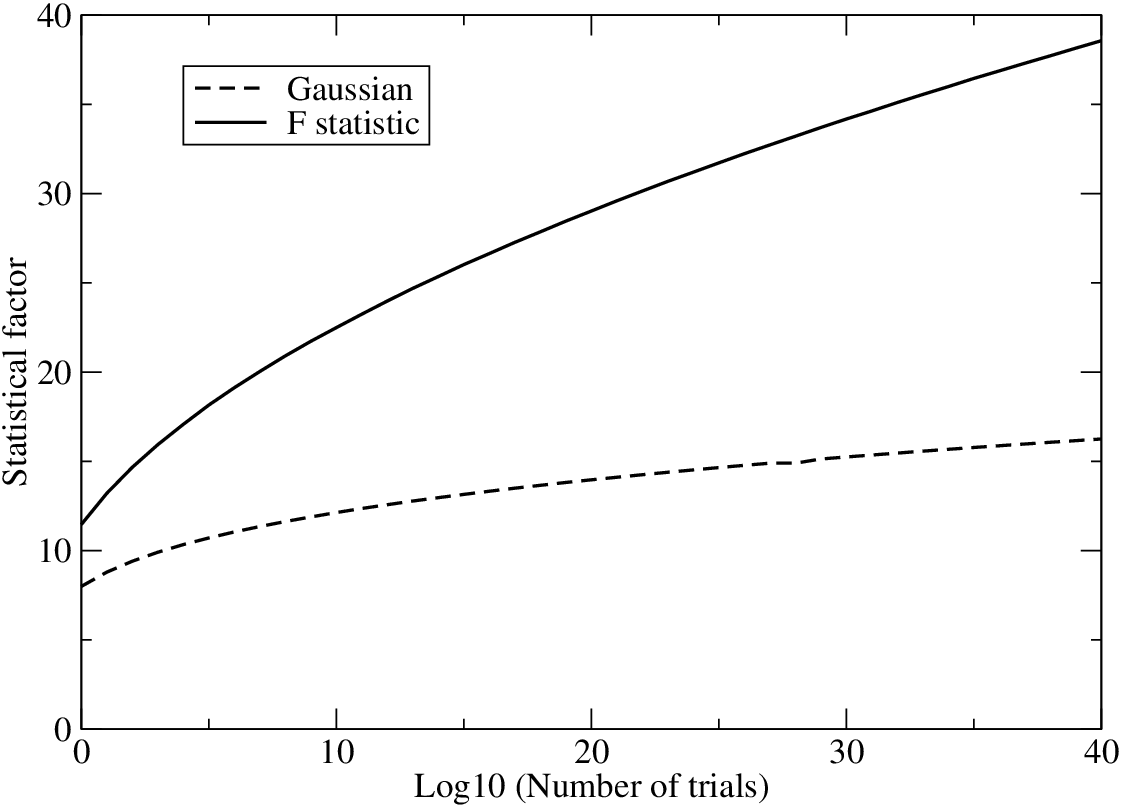
So far we have incorporated the statistical and geometrical factors in Equation (40). For template bank based searches, the sensitivity is further degraded because of the discreteness of the template grid. For a template bank created with a maximum mismatch of $m$ , assuming a cubic grid, the average degradation in the SNR is $(1-m/3)$ . This corresponds to a degradation of $\sqrt{1-m/3}$ in $h_{0}$ which is $\approx 0.95$ for $m=0.3$ .

The next question we need to address is the computational cost and whether it is necessary or worthwhile to do the semi-coherent search (ii). Clearly, for a given amount of data while we ideally want to make the coherent integration time $T_{\rm coh}$ as large as possible, and the number of segments $N_{\rm stacks}$ correspondingly small, the choice of these parameters is dictated by the computational cost. This computational burden is in fact, by far, what limits the search sensitivity (As we just saw, $F_{\rm stat}$ has a very weak dependence on the number of templates; we need to change the number of templates by orders of magnitude before it has an appreciable effect). The bigger effect of reducing the number of templates by better astrophysical modelling or observations is that it allows us to have a larger coherent integration time $T_{\rm coh}$ .

For a given source, we would first like to know if a semi-coherent search would be useful. The obvious answer is: whenever computational cost is an issue, but a more quantitative answer is also easy to get. Let us compare the sensitivities of (i) and (ii) for a given computational cost. Let us assume that the cost for the coherent analysis scales as a power of $T_{\rm obs}$ : $C_{\rm coh}=AT_{\rm obs}^{k}$ for some constants $A$ and $k$ . So if we assume a fixed value of the computational cost $C_{0}$ , then $T_{\rm obs}=(C_{0}/A)^{1/k}$ . Thus, the sensitivity is $h_{0}^{\rm coh}\propto T_{\rm obs}^{-1/2}=(C_{0}/A)^{-1/2k}$ . For a semi-coherent search on the other hand, we have $C_{0}\approx AN_{\rm stacks}T_{\rm coh}^{k}$ (this is true if the cost of combining the different stacks is negligible). In this case we get $T_{\rm coh}=(C_{0}/AN_{\rm stacks})^{1/k}$ . Using $h_{0}^{\rm semi-coh}\propto N^{-1/4}T_{\rm coh}^{-1/2}$ we get

\frac{h_{0}^{\rm semi-coh}}{h_{0}^{\rm coh}}=N_{\rm stacks}^{(2-k)/4k}\,.

(42)

This tells us that a semi-coherent search is not effective (i.e. $h_{0}^{\rm semi-coh}>h_{0}^{\rm coh}$ ) for $k\leq 2$ , and it gets more and more effective for larger $k$ (this conclusion is robust: it is not affected by the approximation of neglecting the cost of the semi-coherent step).

In our present case, recall from equations (17)–(28) that we have very different scalings in the regimes $T_{\rm obs}\gg P_{\rm orb}$ and $T_{\rm obs}\ll P_{\rm orb}$ . So, for binary systems for which the parameters have been sufficiently constrained astronomically and we can afford large integration times, we shall assume that we are better off doing a simple coherent search. For others, a semi-coherent strategy has a much larger impact.²²²² 22 Semi-coherent searches might start becoming more important as soon as we need to start including other parameters, especially frequency derivatives and $\dot{P}_{\rm orb}$ . For each potential source, our strategy is to first estimate the number of templates that are required for a coherent search. With reasonable estimates of available computational resources, and assuming $T_{\rm obs}=2$ years, this determines the maximum coherent integration time $T_{\rm coh}$ that can be analysed. If $T_{\rm coh}$ is not much smaller than $P_{\rm orb}$ , then by the previous argument we assume that the gain in using a semi-coherent search is not significant, and we restrict ourselves to a pure coherent search. On the other hand, if this $T_{\rm coh}$ does turn out to be much less than $P_{\rm orb}$ , then we consider a semi-coherent search and estimate $T_{\rm coh}$ and $N_{\rm stacks}$ (assuming here the cost of the semi-coherent step to be comparable to the coherent step). Equation ((40)) then yields an estimate of the search sensitivity $h_{0}^{\rm sens}$ for each potential source. We take the statistical factor $F_{\rm stat}$ in Equation ((40)) using just the number of templates in the coherent step. There is as yet no systematic study of the semi-coherent metric for binary systems, and this estimate should be updated as soon as these calculations are available. We expect that this approximation will not make a qualitative difference to our final results because of the weak dependence of $F_{\rm stat}$ on the number of templates, but this needs to be verified. In the previous section, we estimated the estimated GW amplitude $h_{0}^{\rm exp}$ from each source, and the ratio $h_{0}^{\rm exp}/h_{0}^{\rm sens}$ can be a useful “detectability” ranking for each source.

In the cases when $P_{\rm orb}$ is essentially unknown, the ranges of $T_{\rm asc}$ and $a_{\rm x}\sin i$ that we have chosen depend on $P_{\rm orb}$ . This means that the parameter space region is not rectangular and thus the template counting equations of Section 4.1 will over-estimate the number of templates significantly, though not by orders of magnitude.

5.3 Numbers of templates

We can now compute the effect on our searches of parameter uncertainty. We will start by considering the effect on the statistical factor $F_{\rm stat}$ , neglecting computational cost issues. In other words, we assume that it is feasible to do a coherent fold. In Tables 2, 3 and 4 we summarize the parameter ranges assumed for the pulsars, bursters and kHz QPO sources respectively. The Tables show the associated $N_{\lambda^{i}}$ for each parameter (for $T_{\rm obs}=2$ years), the resulting total number of templates that must be searched $N_{\rm temp}$ , and the effect on $F_{\rm stat}$ . Figure 9 shows the change in the statistical factor for each source.

In Figure 2, were we showed results for a single template search, each source had $F_{\rm stat}=11.4$ . This meant that we could plot a single detectability threshold curve for each detector. When each source has a different $F_{\rm stat}$ , however, the detectability threshold curves differ for each source. One way of comparing detectability for sources with different noise threshold curves is to plot the ratio of emitted to detectable amplitude: this is the approach that we took for the transients (Figure 5), and that we will adopt when we come to consider computational cost. What we can also do, however, to see the effect, is to scale the predicted amplitude $h_{0}$ by $11.4/F_{\rm stat}$ . Predicted amplitude does not really change, of course, but it is a useful way of visualising the impact of the statistical factor.

Figure 10 shows the impact on the mountain scenario: it should be compared to Figure 2. Only for the most tightly constrained pulsars is detectability largely unchanged: for the majority of sources the detectable amplitude falls by a factor of 2-3 compared to a single template search. Although this does not sound like a great deal, it is sufficient to push all sources except Sco X-1 below the detection threshold for Advanced LIGO broad band²³²³ 23 Sco5 X-1 would also be marginal for Enhanced LIGO, over a restricted frequency range.. The effect on the r-mode scenario, summarized in Tables 2-4, is slightly less severe, leaving Sco X-1, GX 5-1, GX 349+2 and 4U 1820-30 above the detection threshold for Advanced LIGO broad band. The situation is better for the narrow band configuration: although none of the burst oscillation sources remain within range (for any of the emission scenarios considered), several of the kHz QPO sources are still viable. The spins for these sources are poorly constrained. However, the anticipated narrow band configurations (see top panel of Figure 1) have a reasonably broad bandwidth, leaving ample scope for searches.

We can now take the final step and look at the impact of computational constraints on searches involving multiple templates. The available computational power sets the length of data $T_{\rm obs}$ that can feasibly be analysed within a given amount of time. In Table 5 we summarize the impact in the situation where we assume a maximum analysis time of 2 years, assuming that for Advanced LIGO we have computational power 50 times greater than that currently available within the LSC, while for the Einstein Telescope we assume 100 times more computing than at present. These assumptions are, of course, arbitrary, since the computing power that can be applied to future searches depends not just on technology (e.g. Moore’s Law) but also on improvements in data analysis techniques, and of course also on how much money is spent on computing by future projects. We have taken numbers we feel are defensible, but they may turn out to be conservative, especially for the Einstein Telescope.

For the pulsars, computing constraints have little effect on the detectability of the sources; however, these are not likely to be detectable in any case. But for the bursters and the kHz QPO sources, computational constraints lead to a major reduction in the $T_{\rm obs}$ that it is feasible to analyse. For many sources we have to resort to a semi-coherent search, as a coherent fold is no longer possible. Figures 11 and 12 show the effects on detectability for the mountain and r-mode scenarios respectively, taking into account both the change in $F_{\rm stat}$ and the reduced observation times for our assumed computing power.

The additional impact of computational limitation is substantial. For Advanced LIGO’s broad band configuration, only Sco X-1 and 4U 1820-30 (the latter in the r-mode scenario) remain above the detectability threshold. These two sources are also the only two left above the narrow band envelope threshold, although there are other sources just below the envelope that might be detectable if the narrow band configuration were able to push closer to the thermal noise floor.

Parameter uncertainty clearly poses a major problem, even for stars where we have some indication of the spin rate²⁴²⁴ 24 This problem is of course even more pronounced for the accreting neutron stars where we have no indication of spin rate.. If the parameter space volume can be reduced, however, then the statistical and computational restrictions will have less impact. In the following section we will examine this in more detail and consider how best to solve it.

6 Discussion

6.1 Current and future prospects

It is clear from Section 5 that the detection of gravitational waves from accreting neutron stars is a difficult task. The X-ray bright kHz QPO sources suffer from parameter uncertainty, forcing us to look in addition at the much weaker but better constrained burst oscillation sources. The best constrained sources, the accreting millisecond pulsars, are expected to emit at such a low level that they are unlikely to be detectable by second generation detectors. This is particularly depressing since our calculations have been carried out within the context of a fairly optimistic modelling and analysis scenario. We have not as yet considered any additional sources of spin-down, and have also neglected physically reasonable complications such as spin variability which would increase the number of templates still further. Spin variability would of course also lead to decoherence of the signal for sources where we cannot track the spin, reducing integration times to the decoherence time $T_{\rm decoh}$ , defined by

T_{\rm decoh}^{2}\dot{\nu}_{s}=1.

(43)

One can get some idea of the worst case scenario by calculating the $\dot{\nu}_{s}$ that would result if the source were spinning up at the maximal rate due to the accretion torque (Equation 1). The results are given in Table 5: for the bright kHz sources this worst case decoherence time could be $\sim$ 1 week, and this is something that will need to be considered in future studies of detectability.

In order to improve prospects for those sources that are in principle detectable, we clearly need to find ways of improving source constraints and removing computational limitations. In the sections that follow we detail the actions that would lead to the biggest improvements.

6.2 Astronomical observations

The major obstacle to detection by the current and imminent generation of detectors is clearly parameter uncertainty, with spin uncertainty having the largest impact (see Tables 2-4). Astronomical observations might help to constrain source properties.

The single most valuable thing that could be done to improve the current situation is to determine more precisely the NS spin in the bright kHz QPO and burst sources. A substantial archive of high time resolution X-ray data exists for many of these sources from RXTE and its predecessors. However the only deep search for pulsations in the literature is that carried out by Dib et al. (2005) for 4U 1820-30. Serious consideration should be given to carrying out similar analysis for all of the kHz QPO and burst sources, most particularly Sco X-1. Thorough searches for intermittent pulsations, such as those carried out by Casella et al. (2008) and Altamirano et al. (2008), would also be worthwhile.

It may also be possible to find burst oscillations in the kHz QPO sources: five of the sources that we have analysed are known to burst. If a sufficient archive of bursts can be built up from these sources burst oscillations may well be detected either in individual bursts or by stacking power spectra from multiple bursts (the technique used to find weak burst oscillations from EXO 0748-676 (Villarreal & Strohmayer, 2004). We also need to verify the burst oscillation frequencies for the seven sources with tentative or single burst detections, in particular the four that are above the detection threshold for some of the scenarios that we have examined: XB 1254-690, 4U 1916-053, MXB 1730-335 and 4U 0614+09.

Identifying the orbital period can also make a substantial difference to the number of templates searched. Consider for example the difference between the two kHz QPO sources Sco X-1 and GX 5-1. Both are expected to be strong emitters, but Sco X-1 suffers much less from parameter uncertainty than GX 5-1 because the former has a well constrained orbital period. Three of the most promising kHz QPO sources have no orbital constraints (GX 340+0, GX 5-1 and GX 17+2), while a fourth (GX 349+2) has only a relatively weak constraint. Several of the most promising burst oscillation sources also fall into this category: attention should focus on 4U 1608-522, KS 1731-260, 4U 1728-34, 4U 1702-429, and MXB 1730-335, sources that could be detectable in some scenarios. Immense progress has been made in recent years in constraining orbital parameters for LMXBs using optical/IR observations, particularly with the Bowen technique of spectroscopy. Identification of counterparts is often difficult, but there would be a substantial payoff in terms of gravitational wave detection prospects.

6.3 Astrophysical modelling issues

Both burst oscillation frequency and kHz QPO frequency are proxy measures for the stellar spin rate. The precise link to spin for each measure is not clear because in neither case do we understand the mechanism. Astrophysical modelling to pin down the cause of the two phenomena could therefore shed light on the reliability and accuracy of the spin proxy.

Several models have been suggested for burst oscillations. These include global oscillations of the surface layers of the neutron star, large-scale drifting vortices excited by the passage of the flame fronts, or hotspots linked in some way to persistent pulsations. All of the models have shortcomings, and progress towards understanding this phenomenon has to some degree stalled. The situation for the kHz QPOs is however even worse. There are several models, summarized in detail in van der Klis (2006). All involve either orbital motions of material within the disk or disk oscillations, and many also require some mechanism to select preferred radii within the disk. Developing testable predictions that would distinguish between the different models, however, is very difficult. A substantial body of data exists within the RXTE archive to test models if such predictions can be made. The identification of a robust link between kHz QPO frequency and stellar spin would have a major impact in reducing parameter uncertainty for the most promising sources for Advanced LIGO.

6.4 Data analysis and detector issues

In the absence of computational limitations, even taking into account the effect on statistics, there would be up to 8 sources potentially detectable by Advanced LIGO (Figure 10). We therefore need to improve the data analysis tools used for the searches. We need significant improvements in all relevant aspects of the data analysis pipelines: accelerating existing software through improvements to both software algorithms and computer hardware, and also developing other data analysis techniques. The software algorithms being used in the LIGO data analysis software have improved continually over the years since the first LSC publication on periodic waves in 2003; we expect these improvements to continue. It is possible that we may get an improvement of more than a order of magnitude in existing codes over the next several years. The improvements in computer hardware, even just following Moore’s law, will yield an additional factor of about 16 in the next 8 years, i.e. by the time we expect Advanced LIGO to be operating. Furthermore, computing platforms like Einstein@Home allow us to increase the total number of computers available to do the analysis. On top of this, it might also be possible to use special purpose hardware for the periodic wave searches. Most of the analysis involves a large number of relatively simple operations, and it might be quite feasible to design chips which are efficient for these particular calculations. An example of these are the GRAPE special-purpose computers which have proven to be extremely useful in astrophysical N-body simulations (Makino & Taiji, 1995) and in molecular dynamics calculations in condensed matter physics. It is hard to anticipate these developments, but an improvement of 4 or 5 orders of magnitude in effective computing power might be feasible.

Apart from these technical improvements, it is also possible to develop new analysis methods. A good example of this is the cross-correlation method used in the Sco X-1 search (Abbott et al., 2007c). This was neither a matched filter nor a standard time-frequency semi-coherent search. It was instead based on aperture synthesis, i.e. the fact that we have multiple detectors in operation, and that they all see essentially the same GW signal at any given time. This method has so far mostly been used in the stochastic background searches, and is now being adapted to the periodic wave searches (Dhurandhar et al., 2008). Apart from the computational efficiency, this method is also relatively insensitive to the uncertainty in the signal model caused, e.g. by pulsar glitches (though this leads to a correspondingly greater computational cost in any follow-ups that must be done for verifying a detection and for parameter estimation). Further searches using this method, in combination with the other methods discussed in this paper seem to be quite promising, especially given that by the time of Advanced LIGO there will be a third interferometer of comparable sensitivity in Virgo.

In the near term while these improvements are in progress, it seems reasonable to search for some of the brighter sources such as Sco X-1 not at the frequency implied by the kHz QPOs, but rather at lower frequencies corresponding to the sweet spot of the detectors. Not only are the instruments more sensitive at these frequencies, but this is computationally easier and is astrophysically well motivated if the link between the kHz QPO and the spin frequency is not validated.

We conclude this section with a brief discussion of possible Advanced LIGO configurations and some of its implications for our purposes. Figure 13 shows noise curves for three cases: an example broad band configuration with some tuning of the signal recycling cavity optimized for binary neutron star (BNS) inspirals, the envelope of possible narrow band configurations, and the zero-detuned broad band configuration. The zero-detuned curve and the narrow band envelope are the same as in Fig. 1. The BNS curve is relevant because binary neutron star inspirals will be among the key targets for Advanced LIGO and the detector might possibly be operated in this configuration for significant durations. Thus, while BNS signals are not our concern in this paper, it is important to consider the impact of this configuration for our purposes. It is obvious that the BNS curve affects us adversely above $\sim 500\,$ Hz which, as we see from Figure 2 is precisely where the kHz QPO sources are expected to lie.

These curves highlight the importance of spin measurements. For all potential sources with frequencies between, say, $150$ and $2000\,$ Hz, the narrow banding gains us no more than a factor of 2. The best case for narrow banding is then a compelling source whose frequency is very well known and is within this range and is not detectable by the broad-band curve. The other possibility is to employ the zero-detuned noise curve for detection and then use the narrow band curve as a follow up to confirm detection or to increase SNR for extracting better astrophysical information. Given the present uncertainties in the spin frequency, this latter possibility seems to be the best option for detecting periodic waves from LMXBs. This conclusion could change if there turn out to be significant improvements in the narrow band noise curves.

6.5 Conclusions

We have shown that gravitational wave observations of accreting neutron stars will be challenging. It is therefore worthwhile considering what is to be gained from such an effort: what new information gravitational wave observations will bring to the study of these sources.

The input from electromagnetic observations that is required for these searches is primarily on kinematical parameters like spin rates and orbital ephemerides. The gravitational waves that are generated carry information on the orientation and dynamics of the neutron star and its interaction with the accretion disk. The elliptical polarization of the gravitational waves, which will emerge from analysis of the detected signal, determines the orientation of the neutron-star spin axis. The degree of alignment of this with the inferred disk orientation, especially for the slower-spinning (presumably younger) systems, will constrain models of binary evolution and the formation of the NS.

In systems where observations and modelling constrain the NS spin to a relatively narrow range, the GW frequency will determine whether the r-mode or mountain scenario, or indeed some other scenario, is the appropriate one. The GW amplitude will then determine the degree of mass asymmetry (mountains) or the size of the velocity field (r-modes). In both cases this will open for the first time a wealth of opportunities for studying the physics of NS interiors.

For all detected systems, the measured GW amplitude and frequency will tell us how much angular momentum is being carried away in GWs; by measuring or limiting the rate of change of the GW frequency we can then infer the rate at which angular momentum is being accreted from the disk. This will be an important constraint on models of the disk and the NS magnetic field.

Clearly, if GW searches turn up signals in unexpected places in parameter space, this will challenge prevailing models for these systems. For example, if the GW frequency equals the X-ray pulsation frequency instead of twice or four thirds its value, then this might imply that the pulsation frequency is actually twice the true spin frequency.

Even in the worst case, where a sufficiently sensitive search fails to detect GWs at the expected amplitude, the negative result could eliminate the GW option for spin balance and demonstrate that this somehow resulted from a propeller-type torque from the NS’s magnetic field. Of course, one would have to have confidence that the GWs were not coming out at a different frequency, so the search would have to include that as a parameter.

The additional astronomical input that could make the difference between detecting or not detecting GWs could come from a variety of observations. Clearly, long-term X-ray timing is highly desirable, and here it is disappointing that the future of RXTE is limited and no X-ray mission with comparable capabilities seems to be planned for the period before Advanced LIGO comes online. Thorough exploitation of the RXTE data archive is therefore especially important. On the other hand, sensitive radio observations of X-ray systems in quiescence may provide unexpected information, and this will be easier with arrays like the Square Kilometre Array and its pathfinders.

7 Acknowledgements

We would like to thank Alan Levine for advice on ASM countrates, Jake Hartman for advice on the effects of positional uncertainty on pulsar timing, Reinhard Prix for help with the computational cost estimates, Alberto Vecchio and Chris Messenger for discussions regarding the parameter space metric, and Maria Alessandra Papa, Mike Landry and Graham Woan for useful comments on a draft of this paper. We are grateful to Rana Adhikari, Peter Fritschel, Gregg Harry, Bangalore Sathyaprakash, David Shoemaker, Kentaro Somiya and Ken Strain for pointing us to Bench and for valuable discussions related to the Advanced LIGO noise spectrum. We thank Rana Adhikari also for providing us with the Enhanced LIGO noise curve. ALW would like to thank the Kavli Institute for Theoretical Physics for hospitality during a KITP/MPA postdoctoral exchange visit, when this work was started. BK is grateful to the LSC continuous-waves data analysis group for valuable discussions. LB acknowledges support from the National Science Foundation via grants PHY 05-51164 and AST 02-05956. BK and BFS acknowledge the support of the DFG’s special research centre SFB/Transregio 7 “Gravitational Wave Astronomy”.

References

Abbott et al. (2004) Abbott B. et al., 2004, Phys. Rev. D 69, 182004
Abbott et al. (2005b) Abbott B. et al., 2005b, Phys. Rev. Lett. 94, 181103
Abbott et al. (2007b) Abbott B. et al., 2007b, Phys. Rev. D 76, 042001
Abbott et al. (2005a) Abbott B. et al., 2005a, Phys. Rev. D 72, 102004
Abbott et al. (2008) Abbott B. at al., 2008, Phys. Rev. D 77, 022001
Abbott et al. (2007a) Abbott B. et al., 2007a, Phys. Rev. D 76, 082001
Abbott et al. (2007c) Abbott B. et al., 2007c, Phys. Rev. D 76, 082003
Altamirano et al. (2005) Altamirano, D., van der Klis, M., Méndez, M., Migliari, S., Jonker, P.G., Tiengo, A., Zhang, W. 2005, ApJ, 633, 358
Altamirano et al. (2008) Altamirano D., Casella P., Patruno A., Wijnands R., van der Klis M., 2008, ApJ, 674, L45
Anderson et al. (1997) Anderson, S.F., Margon, B., Deutsch, E.W., Downes, R.A., Allen, R.G., 1997, ApJ, 482, L69
Andersson, Kokkotas & Stergioulas (1999) Andersson N., Kokkotas K.D., Stergioulas N. 1999, ApJ, 516, 307
Andersson et al. (2000) Andersson N., Jones D.I., Kokkotas K.D., Stergioulas N. 2000, ApJ, 534, L75
Andersson & Kokkotas (2001) Andersson N., Kokkotas K.D., 2001, Int. J. Mod. Phys., 10, 381
Andersson, Jones & Kokkotas (2002) Andersson N., Jones D.I., Kokkotas K.D. 2002, MNRAS, 337, 1224
Andersson et al. (2005) Andersson N., Glampedakis K., Haskell B., Watts A.L. 2005, MNRAS, 361, 1153
Arras et al. (2003) Arras P., Flanagan E.E., Morsink S.M., Schenk A.K., Teukolsky S.A., Wasserman I., 2003, ApJ, 591, 1129
Astone et al. (2005) Astone P. et al. 2005, Class. Quant. Grav., 22, S1243-S1254
Astone et al. (2002) Astone P. et al. 2002, Phys.Rev.D, 65, 042003
Augusteijn et al. (1998) Augusteijn T., van der Hooft F., de Jong J.A., van Kerkwijk M.H., van Paradijs J. 1998, A&A, 332, 561
Ballantyne & Strohmayer (2004) Ballantyne D.R., Strohmayer T.E., 2004, ApJ, 602, L105
Baraffe & Kolb (2000) Baraffe I., Kolb U, 2000, MNRAS, 318, 354
Barnes et al. (2007) Barnes A.D., Casares J., Cornelisse R., Charles P.A., Steeghs D., Hynes R.I., O’Brien K., 2007, MNRAS, 380, 1182
Barret, Olive & Miller (2005) Barret D., Olive J.-F., Miller M.C. 2005, MNRAS, 361, 855
Barret, Boutelier & Miller (2008) Barret D., Boutelier M., Miller M.C., 2008, MNRAS, 384, 1519
Barziv et al. (1997) Barziv O., Kuulkers E., Méndez M., van der Hooft F., Groot P.J., van der Klis M., Kemper C., van Paradijs J. 1997, A&A, 325, 1035
Berendsen et al. (2000) Berendsen S.G.H., Fender R., Kuulkers E., Heise K., van der Klis M. 2000, MNRAS, 318, 599
Bhattacharyya et al. (2006) Bhattacharyya S., Strohmayer T.E., Markwardt C.B., Swank J.H. 2006, ApJ, 639, L31
Bhattacharyya (2007) Bhattacharyya S. 2007, MNRAS, 377, 198
Bildsten (1998) Bildsten L., 1998, ApJ, 501, L89
Bildsten & Chakrabarty (2001) Bildsten L. & Chakrabarty, D., 2001, ApJ, 557, 292
Bodghee et al. (2005) Bodghee A., Mowlavi N., Kuulkers E., Wijnands R., Shaw S.E., Courvoisier T., Markwardt C., Oosterbroek T., Orr A., Paizis A., Ebisawa K., Kretschmar P. 2005, Atel 592
Boirin et al. (2000) Boirin L., Barret D., Olive J., Bloser P., Grindlay J., 2000, A&A, 361, 121
Bondarescu, Teukolsky & Wasserman (2007) Bondarescu R., Teukolsky S.A., Wasserman I., 2007, Phys. Rev. D 76, 64019
Boutloukos et al. (2006) Boutloukos S., van der Klis M., Altamirano D., Klein-Wolt M., Wijnands R., Jonker P.G., Fender R.P. 2006, ApJ, 653, 1435
Bradshaw, Fomalont & Geldzahler (1999) Bradshaw C.F., Fomalont E.B., Geldzahler B.J. 1999, ApJ, 512, 121
Bradt & McClintock (1983) Bradt H.V.D., McClintock J.E. 1983, Ann. Rev. Astron. Astrophys. 21, 13
Brady et al. (1998) Brady P.R., Creighton T., Cutler C., Schutz B. 1998, Phys. Rev. D. 57, 1
Brady & Creighton (2000) Brady P.R., Creighton T., 2000, Phys. Rev. D, 61, 082001
Brandt et al. (1992) Brandt S., Castro-Tirado A.J., Lund N., Dremin V., Lapshov I., Sunyaev R.A. 1992, A&A, 262, L15
Buonanno & Chen (2002) Buonanno, A & Chen, Y 2002, Phys.Rev.D, 65, 042001
Burderi et al. (2007) Burderi L., di Salvo T., Lavagetto G., Menna M.T., Papitto A., Riggio A., Iaria R., d’Antona F., Robba N.R., Stella L. 2007, ApJ, 657, 961
Callanan et al. (2002) Callanan P.J., Curran P., Filippenko A.V., Garcia A.V., Margon B., Deutsch E., Anderson S., Homer L., Fender R.P. 2002, ApJ, 574, L143
Casares, Charles & Kuulkers (1998) Casares J., Charles P., Kuulkers E. 1998, ApJ, 493, L39
Casares et al. (2002) Casares J., Dubus G., Shahbaz T., Zurita C., Charles P.A. 2002, MNRAS, 329, 29
Casares et al. (2006) Casares J., Cornelisse R., Steeghs D., Charles P.A., Hynes R.I., O’Brien K., Strohmayer T.E. 2006, MNRAS, 373, 1235
Casella et al. (2008) Casella P., Altamirano D., Patruno A., Wijnands R., van der Klis M., 2008, ApJ, 674, L41
Chabrier & Baraffe (2000) Chabrier G., Baraffe I., 2000, ARA&A, 38, 337
Chabrier et al. (2000) Chabrier G., Baraffe I., Allard F., Hauschildt P., 2000, ApJ, 542, 464
Chakrabarty et al. (2003) Chakrabarty D., Morgan E., Muno M., Galloway D., Wijnands R., van der Klis M., Markwardt C., 2003, Nature, 424, 42
Chevalier & Ilovaisky (1998) Chevalier C., Ilovaisky S.A. 1998, IAUC 6806.
Chou & Grindlay (2001) Chou, Y., Grindlay, J.E. 2001, ApJ, 563, 934
Chou, Grindlay & Bloser (2001) Chou Y., Grindlay J.E., Bloser P.F. 2001, ApJ, 549, 1144
Chou et al. (2008) Chou Y., Chung Y., Hu C.P., Yang T.C., 2008, ApJ, 678, 1316
Christian & Swank (1997) Christian D.J., Swank J.H. 1997, ApJS, 109, 177
Cook, Shapiro & Teukolsky (1994) Cook, G. B., Shapiro, S. L. & Teukolsky, S. A. 1994, ApJ, 423, L117
Cooke & Ponman (1991) Cooke B.A., Ponman T.J. 1991, A&A, 244, 358
Cominsky & Wood (1984) Cominsky L.R., Wood K.S., 1984, ApJ, 283, 765
Cornelisse et al. (2007) Cornelisse R., Casares J., Steeghs D., Barnes A.D., Charles P.A., Hynes R.I., O’Brien K., 2007, MNRAS, 375, 1463
Courvoisier et al. (1986) Courvoisier T.J.-L., Parmar A.N., Peacock A., Pakull M. 1986, ApJ, 309, 265
Cutler (2002) Cutler C. 2002, Phys. Rev. D., 66, 084025
Cutler et al. (2005) Cutler C., Gholami I., Krishnan B. 2005, Phys. Rev. D, 72, 042004
Cutler & Schutz (2005) Cutler C., Schutz B.F. 2005, Phys.Rev.D, 72, 063006
Degenaar et al. (2007) Degenaar N. et al., 2007, Atel 1106
Deloye & Bildsten (2003) Deloye C.J., Bildsten L., 2003, ApJ, 598, 1217
Deutsch et al. (1999) Deutsch E.W., Margon B., Anderson S.F., Wachter S., Goss W.M. 1999, ApJ, 524, 406
Dhurandhar & Vecchio (2001) Dhurandhar S.V., Vecchio A., 2001, Phys. Rev. D 63, 122001
Dhurandhar et al. (2008) Dhurandhar S.V., Krishnan B., Mukhopadhyay H., and Whelan J., Phys. Rev. D 77, 082001
Dib et al. (2005) Dib, R., Ransom, S.M., Ray, P.S., Kaspi, V.M., Archibald, A.M. 2005, ApJ, 626, 333.
di Salvo et al. (2001) di Salvo T., Méndez M., van der Klis M., Ford E., Robba N.R. ApJ, 546, 1107
di Salvo, Méndez & van der Klis (2003) di Salvo T., Méndez M., van der Klis M. 2003, A&A, 406, 177
Dubus et al. (1999) Dubus G., Lasota J.-P., Hameury J.-M., Charles P., 1999, MNRAS, 303, 139
Falanga et al. (2005) Falanga M., Kuiper L., Poutanen J., Bonning E.W., Hermsen W., di Salvo T., Goldoni P., Goldwurm A., Shaw S.E., Stella L. 2005, A&A, 444, 15
Fender & Hendry (2000) Fender R.P., Hendry M.A., 2000, MNRAS, 317, 1
Ford et al. (1997) Ford E., Kaaret P., Tavani M., Barret D., Bloser P., Grindlay J., Harmon B.A., Paciesas W.S., Zhang S.N. 1997, ApJ, 475, L123
Ford et al. (1998) Ford E.C., van der Klis M., van Paradijs J., Méndez M., Wijnands R., Kaaret P., 1998, ApJ, 508, L155
Ford et al. (2000) Ford E.C., van der Klis M., Méndez M., Wijnands R., Homan J., Jonker P.G., van Paradijs J., 2000, ApJ, 537, 368
Fox et al. (2001) Fox D.W., Lewin W.H.G., Rutledge R.E., Morgan E.H., Guerriero R., Bildsten L., van der Klis M., van Paradijs J., Moore C.B., Dotani T., Asai K. 2001, MNRAS, 321, 776
Fox & Kulkarni (2004) Fox D.B., Kulkarni S.R., 2004, Atel 354
Fox (2005) Fox D.B. 2005, Atel 526, 1
Freire et al. (2008) Freire, P. C. C., Ransom, S. M., Begin, S., Stairs, I. H., Hessels, J. W. T., Frey, L. H., Camilo, F. 2008, ApJ, 675, 670
Galloway et al. (2001) Galloway D., Chakrabarty D., Muno M., Savov P., 2001, ApJ, 549, L85
Galloway et al. (2002) Galloway D., Chakrabary D., Morgan E.H., Remillard R.A. 2002, ApJ, 576, L137
Galloway, Cumming & Chakrabarty (2004) Galloway D., Cumming A., Chakrabarty D., 2004, AAS/High Energy Astrophysics Division, 8,
Galloway et al. (2005) Galloway D.K., Markwardt C.B., Morgan, E.H., Chakrabarty, D., Strohmayer, T.E., 2005, ApJ, 622, L45
Galloway (2006) Galloway D.K., Accretion powered millisecond pulsar outbursts, 2006, in ‘The transient Milky Way: a perspective for MIRAX’, eds F. D’Amico, J. Braga & R. Rothschild, AIP Conf. Proc, 840, 50
Galloway & Cumming (2006) Galloway D.K., Cumming A. 2006, ApJ, 652, 559
Galloway et al. (2006) Galloway D.K., Psaltis D., Muno M.P., Chakrabarty D. 2006, ApJ, 639, 1033
Galloway et al. (2007a) Galloway D.K., Morgan E.H. Krauss M.I., Kaaret P., Chakrabarty D. 2007, ApJ, 654, L73
Galloway et al. (2008) Galloway D.K., Muno M.P., Hartman J.M., Savov P., Psaltis D., Chakrabarty D. 2008, ApJS submitted, astro-ph/0608259.
Galloway, Özel & Psaltis (2008) Galloway D.K., Özel F., Psaltis D., MNRAS, 387, 268
Garcia et al. (1999) Garcia M.R., Callanan P.J., McCarthy J., Eriksen K., Hjellming R.M. 1999, ApJ, 518, 422
Gavriil et al. (2007) Gavriil F.P., Strohmayer T.E., Swank J.H., Markwardt C.B., 2007, ApJ, 669, L29
Ghosh & Lamb (1978) Ghosh P., Lamb F. 1978, ApJ, 223, L83
Giacconi et al. (1967) Giacconi R., Gorenstein P., Gursky H., Usher P.D., Waters J.R., Sandage A., Osmer P., Peach J.V. 1967, ApJ, 148, L129
Gierliński & Done (2002) Gierliński M., Done C., 2002, MNRAS, 331, L47
Gierliński, Done & Barret (2002) Gierliński M., Done C., Barret D., 2002, MNRAS, 331, 141
Gierliński & Poutanen (2005) Gierliński M., Poutanen J., 2005, MNRAS, 343, 1301
Giles et al. (2002) Giles A., Hill K., Strohmayer T., Cummings N., 2002, ApJ, 568, 279
Giles et al. (2005) Giles A.B., Greenhill J.G., Hill K.M., Sanders E. 2005, MNRAS, 361, 1180
Gottlieb, Wright & Liller (1975) Gottlieb E.W., Wright E.L., Liller W., 1975, ApJ, 195, L33
Gottwald et al. (1991) Gottwald M., Steinle H., Pietsch W., Graswer U. 1991, Astronomy & Astrophysics Supplement Series, 89,
Greenhill, Giles & Hill (2002) Greenhill J.G., Giles A.B., Hill K.M. 2002, IAUC 7889, 1
Grindlay & Liller (1978) Grindlay, J.G., Liller, W. 1978, ApJ, 220, L127
Hartman et al. (2003) Hartman J., Chakrabarty D., Galloway D., Muno M., Savov P., Méndez M., van Straaten S., di Salvo T., 2003, AAS/High Energy Astrophysics Division, 7,
Hartman et al. (2008) Hartman J., Patruno A., Chakrabarty D., Kaplan D.L., Markwardt C.B., Morgan E.H., Ray P.S., van der Klis M., Wijnands R. 2008, ApJ, 675, 1468
Hasinger & van der Klis (1989) Hasinger, G., van der Klis M., 1989, A&A, 225, 79
Haskell, Jones & Andersson (2006) Haskell B., Jones D.I., Andersson N. 2006, MNRAS, 373, 1423
Haskell et al. (2008) Haskell B., Samuelsson L., Glampedakis K., Andersson N., 2008, MNRAS, 385, 531
Heasley et al. (2000) Heasley, J.N., Janes, K.A., Zinn, R., Demarque, P., da Costa, G.S., Christian, C.A. 2000, AJ, 120, 879
Hertz et al. (1992) Hertz P., Vaughan B., Wood K.S., Norris J.P., Mitsuda K., Michelson P.F., Dotani T. 1992, ApJ, 396, 201
Hessels et al. (2006) Hessels J.W.T., Ransom S.M., Stairs I.H., Freire P.C.C., Kaspi V.M., Camilo F. 2006, Science, 311, 1901
Hessels et al. (2007) Hessels J.W.T., Ransom S.M., Stairs I.H., Kaspi, V. M. & Freire P.C.C. 2007, ApJ, 670, 363
Heyl (2002) Heyl J. 2002, ApJ, 574, L57
Heyl (2004) Heyl J.S. 2004, ApJ, 600, 939
Homan et al. (1999) Homan J., Méndez M., Wijnands R., van der Klis M., van Paradijs J., 1999, ApJ, 513, L119
Homan et al. (2002) Homan J., van der Klis M., Jonker P., Wijnands R., Kuulkers E., Méndez M., Lewin W., 2002, ApJ, 568, 878
Homer et al. (2001) Homer L., Deutsch E.W., Anderson S.F., Margon B. 2001, AJ, 122, 2627
Horne, Wade & Szkody (1986) Horne K., Wade R.A., Szkody P., 1986, MNRAS, 219, 791
Hynes et al. (2006) Hynes R.I., Horne K., O’Brien K., Haswell C.A., Robinson E.L., King A.R., Charles P.A., Pearson K.J., 2006, ApJ, 648, 1156
Iaria et al. (2004) Iaria R., di Salvo T., Robba N.R., Burderi L., Stella L., Frontera F., van der Klis M. 2004, ApJ, 600, 358
Iaria et al. (2006) Iaria R., di Salvo T., Lavagetto G., Robba N.R., Burderi L. 2006, ApJ, 647, 1341
Iaria et al. (2007) Iaria R., di Salvo T., Lavagetto G., d’Aí A., Robba N.R. 2007, A&A, 464, 291
in’t Zand et al. (2003) in’t Zand J.J.M., Kuulkers E., Verbunt F., Heise J., Cornelisse R. 2003, A&A, 411, L487
in’t Zand, Jonker & Markwardt (2007) in’t Zand J.J.M., Jonker P.G., Markwardt C.B., 2007, A&A, 465, 953
Jaranowski, Królak & Schutz (1998) Jaranowski P., Królak A, Schutz B.F. 1998, Phys. Rev. D 58, 063001
Johnston, Fender & Wu (1999) Johnston H.M., Fender R., Wu K. 1999, MNRAS, 308, 415
Johnston et al. (2001) Johnston H.M., Wu K., Fender R., Cullen J.G. 2001, MNRAS, 328, 1193
Jongert & van der Klis (1996) Jongert H.C., van der Klis M. 1996, A&A, 310, 474
Jonker et al. (1998) Jonker P.G., Wijnands R., van der Klis M., Psaltis D., Kuulkers E., Lamb F.K. 1998, ApJ, 499, L191
Jonker et al. (2000) Jonker P., van der Klis M., Wijnands R., Homan J., van Paradijs J., Méndez M., Ford E., Kuulkers E., Lamb F., 2000, ApJ, 537, 374
Jonker et al. (2002) Jonker P., Méndez M., van der Klis M., 2002, MNRAS, 336, L1
Jonker et al. (2002) Jonker P., van der Klis M., Homan J., Méndez M., Lewin W., Wijnands R., Zhang W., 2002, MNRAS, 333, 665
Jonker, Nelemans & Bassa (2007) Jonker P.G., Nelemans G., Bassa C.G. 2007, MNRAS, 374, 999
Juett, Psaltis & Chakrabarty (2001) Juett A.M., Psaltis D., Chakrabarty D. 2001, ApJ, 560, L59
Kaaret et al. (2002) Kaaret P., in’t Zand J., Heise J., Tomsick J., 2002, ApJ, 575, 1018
Kaaret et al. (2006) Kaaret P., Morgan E.H., Vanderspek R., Tomsick J. 2006, ApJ, 638, 963
Kaaret et al. (2007) Kaaret P., Prieskorn Z., in’t Zand J.J.M., Brandt S., Lund N., Mereghetti S., Götz D., Kuulkers E., Tomsick J.A. 2007, ApJ, 657, L97
Kawai & Suzuki (2005) Kawai N., Suzuki M. 2005, Atel, 534
King, Kolb & Burderi (1996) King A.R., Kolb U., Burderi L., 1996, ApJ, 464, L127
Kinney & Mendell (2003) Kinney J.B., Mendell G. 2003, Phys. Rev. D, 67. 024032
Klein-Wolt et al. (2007a) Klein-Wolt M., Wijnands R., Swank J.H., Markwardt C.B., 2007, Atel 1065
Klein-Wolt et al. (2007b) Klein-Wolt M., Maitra D., Wijnands R., Swank J.H., Markwardt C.B., Bailyn C., 2007, Atel 1070
Klein-Wolt et al. (2007c) Klein-Wolt M., Wijnands R., Swank J.H., Markwardt C.B., 2007, Atel 1075
Kolb, King & Baraffe (2001) Kolb U., King A.R., Baraffe I., 2001, MNRAS, 321, 544
Krauss et al. (2005) Krauss M.I., Wang Z., Dullighan A., Juett A.M., Kaplan D., Chakrabarty D., van Kerkwijk M.H., Steeghs D., Jonker P.G., Markwardt C.B. 2005, ApJ, 627, 910
Krauss et al. (2006) Krauss M.I., Juett A.M., Chakrabarty D., Jonker P.G., Markwardt C.B. 2006, Atel 777
Krimm et al. (2007) Krimm H.A. et al., 2007, ApJ, 668, L147
Krishnan et al. (2004) Krishnan B. et al. 2004, Phys. Rev. D, 70, 082001
Kuulkers et al. (1995) Kuulkers E., van der Klis M., van Paradijs J. 1995, ApJ, 450, 748
Kuulkers et al. (1997) Kuulkers E., van der Klis, Oosterbroek T., van Paradijs J., Lewin W.H.G. 1997, MNRAS, 287, 495
Kuulkers et al. (2002) Kuulkers E., Homan J., van der Klis M., Lewin W.H.G., Méndez M. 2002, A&A, 382, 947
Kuulkers et al. (2003) Kuulkers E., den Hartog P.R., in’t Zand J.J.M., Verbunt F.W.M., Harris W.E., Cocchi M. 2003, A&A, 399, 663
Kuznetsov (2002) Kuznetsov S.I. 2002, Astronomy Letters, 28, 73
Lattimer & Prakash (2007) Lattimer J.M., Prakash M. 2007, Physics Reports, 442, 109
Levin (1999) Levin Y. 1999, ApJ, 517, 328
Levine et al. (1996) Levine A.M., Bradt H., Cui W., Jernigan J.G., Morgan E.H., Remillard R., Shirey R.E., Smith D.A., 1996, ApJ, 469, L33
Levine & Corbet (2006) Levine A.M., Corbet R. 2006, Atel 940
Linares et al. (2005) Linares M., van der Klis M., Altamirano D., Markwardt C.B. 2005, ApJ, 634, 1250
Lochner & Roussel-Dupre (1994) Lochner J.C., Roussel-Dupre D. 1994 ApJ, 435, 840
Makino & Taiji (1995) Makino J. and Taiji M., 1995, Proc. 1995 ACM/IEEE conference on supercomputing, 63.
Markwardt, Strohmayer & Swank (1999a) Markwardt C., Strohmayer T., Swank J., 1999, ApJ, 512, L125
Markwardt et al. (1999b) Markwardt C.B., Marshall F.E., Swank J.H., Cui W. 1999, IAUC 7300, 1
Markwardt et al. (2002) Markwardt C., Swank J., Strohmayer T., in’t Zand M., Marshall F., 2002, ApJ, 575, L21
Markwardt, Juda & Swank (2003) Markwardt C., Juda, M., Swank J., 2003, IAU Circ., 8095, 2
Markwardt & Swank (2003) Markwardt C., Swank J., 2003, IAU Circ., 8144
Markwardt et al. (2007) Markwardt C.B., Klein-Wolt M., Swank J.H., Wijnands R. 2007, Atel 1068
Martí et al. (1998) Martí J., Mirabel I.F., Rodríguez L.F., Chaty S. 1998, A&A, 332, L45
Meers (1988) Meers B.J. 1988, Phys. Rev. D, 38, 2317
Meinshausen, Bickel & Rice (2007) Meinshausen N., Bickel P. & Rice J. 2007, arXiv:0712.1663
Melatos & Payne (2005) Melatos A., Payne D.J.B. 2005, ApJ, 623, 1044
Méndez et al. (1998a) Méndez M., van der Klis M., van Paradijs J., Lewin, W.H.G., Vaughan B., Kuulkers, E., Zhang, W., Lamb, F.K., Psaltis, D. 1998, ApJ, 494, L65
Méndez et al. (1998b) Méndez M., van der Klis M., Wijnands R., Ford E., van Paradijs J., Vaughan B., 1998, ApJ, 505, L23
Méndez, van der Klis & van Paradijs (1998) Méndez M., van der Klis M., van Paradijs J. 1998, ApJ, 506, L117
Méndez & van der Klis (1999) Méndez M., van der Klis M., 1999, ApJ, 517, L51
Méndez & van der Klis (2000) Méndez M., van der Klis M., 2000, MNRAS, 318, 938
Méndez & Belloni (2007) Méndez M., Belloni T., 2007, MNRAS, 381, 790
Messenger & Woan (2007) Messenger C., Woan G., 2007, Class. Quant. Grav., 24, 469
Middleditch & Priedhorsky (1986) Middleditch J., Priedhorsky W., 1986, ApJ, 306, 230
Migliari et al. (2003) Migliari S., van der Klis M., Fender R., 2003, MNRAS, 345, L35
Migliari et al. (2004) Migliari, S., Fender, R.P., Rupen, M., Wachter, S., Jonker, P.G., Homan, J., van der Klis, M. 2004, MNRAS, 351, 186
Migliari & Fender (2006) Migliari S., Fender R.P., 2006, MNRAS, 366, 79
Migliari et al. (2006) Migliari S., Tomsick J.A., Maccarone T.J., Gallo E., Fender R.P., Nelemans G., Russell D.M. 2006, 643, L41
Mignani et al. (2002) Mignani R.P., Chaty S., Mirabel I.F., Mereghetti S., 2002, A&A, 389, L11
Moore et al. (2000) Moore C.B., Rutledge R.E., Fox D.W., Guerriero R.A., Lewin W.H.G., Fender R., van Paradijs J. 2000, ApJ, 532, 1181
Motch et al. (1987) Motch C., Pedersen H., Beuermann K., Pakull M.W., Courvoisier T.J.-L. 1987, ApJ, 313, 792.
Muno et al. (2000) Muno M.P., Fox D.W., Morgan E.H., Bildsten L. 2000, ApJ, 542, 1016
Muno et al. (2001) Muno M., Chakrabarty D., Galloway D., Savov P., 2001, ApJ, 553, L157
Muno, Özel & Chakrabarty (2002) Muno M.P., Özel F., Chakrabarty D., 2002, ApJ, 581, 550
Muno, Remillard & Chakrabarty (2002) Muno M.P., Remillard R.A., Chakrbarty D., 2002, ApJ, 568, L35
Muno, Baganoff & Arabadijs (2003) Muno M.P., Baganoff F.K., Arabadijs J.S. 2003, ApJ, 598, 474
Murdin et al. (1980) Murdin P., Jauncey D.L, Lerche I., Nicolson G.D., Kaluzienski L.J., Holt S.S., Haynes R.F. 1980, A&A, 87, 292
Natalucci et al. (1999) Natalucci L., Cornelisse R., Bazzano A., Cocchi M., Ubertini P., Heise J., in’t Zand J., Kuulkers E., 1999, ApJ, 523, L45
Nayyar & Owen (2006) Nayyar M., Owen B.J. 2006, Phys. Rev. D, 73, 084001
Nelemans et al. (2004) Nelemans G., Jonker P.G., Marsh T.R., van der Klis M. 2004, MNRAS, 348, L7
Nelemans, Jonker & Steeghs (2006) Nelemans G., Jonker P.G., Steeghs D., 2006, MNRAS, 370, 255
O’Neill et al. (2002) O’Neill P.M., Kuulkers E., Sood R.K., van der Klis M. 2002, MNRAS, 336, 217
Oosterbroek et al. (1995) Oosterbroek T., van der Klis M., Kuulkers E., van Paradijs J., Lewin W.H.G. 1995, A&A, 297, 141
Oosterbroek et al. (2001) Ooesterbroek T., Parmar A.N., Sidoli L., in’t Zand J.J.M., Heise J. 2001, A&A, 376, 532
Orosz & Kuulkers (1999) Orosz J.A., Kuulkers E. 1999, MNRAS, 305, 132
Ortolani, Barbuy & Bica (1994) Ortolani S., Barbuy B., Bica E., 1994, A&A, 108, 653
Owen (1996) Owen, B.J. 1996, Phys. Rev. D, 53, 6749
Owen et al. (1998) Owen B.J., Lindblom L., Cutler C., Schutz B.F., Vecchio A., Andersson N., 1998, Phys. Rev. D, 58, 084020
Paizis et al. (2005) Paizis A., Nowak M.A., Wilms J., Courvoisier T.J.-L., Ebisawa K., Rodriguez J., Ubertini P. 2005, A&A, 444, 357
Papaloizou & Pringle (1978) Papaloizou J., Pringle J.E. 1978, MNRAS, 184, 501
Papitto et al. (2007) Papitto A., di Salvo T., Burderi L., Menna M.T., Lavagetto G., Riggio A. 2007, MNRAS, 375, 971
Papitto et al. (2008) Papitto A., Menna M.T., Burderi L., di Salvo T., Riggio, A., 2008, MNRAS, 383, 411
Parmar et al. (1986) Parmar A.N., White N.E., Giommi P., Gottwald M. 1986, ApJ, 308, 199
Patruno et al. (2008) Patruno A., Altamirano D., Hessels J.W.T., Casella P., Wijnands R., van der Klis M., 2008, arXiv:0801.1031
Payne & Melatos (2006) Payne D.J.B., Melatos A. 2006, ApJ, 641, 471
Penninx (1989) Penninx W., 1989, in: The 23rd ESLAB Symposium on Two Topics in X-ray Astronomy. Volume 1: X-ray Binaries, p. 185-196, ESA.
Penninx et al. (1993) Penninx W., Zwarthoed G.A.A., van Paradijs J., van der Klis M., Lewin W.H.G., Dotani T. 1993, A&A, 267, 92
Piro & Bildsten (2005) Piro A.L., Bildsten L. 2005, ApJ, 629, 438
Pooley et al. (2002) Pooley D., Lewin W.H.G., Verbunt F., Homer L., Margon B., Gaensler B.M., Kaspi V.M., Miller J.M., Fox D.W., van der Klis M. 2002, ApJ, 573, 184.
Podsiadlowski, Rappaport & Pfahl (2002) Podsiadlowski P., Rappaport S., Pfahl E.D. 2002, ApJ, 565, 1107.
Prix & Itoh (2005) Prix R., Itoh Y. 2005, Class. Quant. Grav., 22, S1003
Prix (2007) Prix R., 2007, Class. Quant. Grav., 24, S481
Prix (2007b) Prix R., 2007, Phys. Rev. D 75, 023004
Rappaport & Joss (1984) Rappaport S., Joss P.C., 1984, ApJ, 283, 232
Rappaport et al. (1987) Rappaport S., Ma C.P., Joss P.C., Nelson L.A. 1987, ApJ, 322, 842
Ransom et al. (2003) Ransom S.M., Cordes J.M., Eikenberry S.S., 2003, ApJ, 589, 911
Ransom et al. (2005) Ransom S.M., Hessels, J. W. T., Stairs, I. H., Friere, P. C. C., Camilo, F., Kaspi, V. M., Kaplan, D. L. 2005, Science, 307, 892
Remillard (2004) Remillard R. 2004, Atel 357.
Retter et al. (2002) Retter A., Chou Y., Bedding T.R., Naylor T. 2002, MNRAS, 330, L37
Revnivtsev & Sunyaev (2002) Revnivtsev M.G., Sunyaev R. 2002, Astronomy Letters, 28, 19
Riggio et al. (2007) Riggio A., di Salvo T., Burderi L., Iaria R., Papitto A., Menna M.T., Lavagetto G., 2007, MNRAS, 382, 1751
Riggio et al. (2008) Riggio A., di Salvo T., Burderi L., Menna M.T., Papitto A., Iaria R., Lavagetto G., 2008, ApJ, 678, 1273
Rupen, Dhawan & Mioduszewski (2003) Rupen M.P., Dhawan V., Mioduszewski A.J., 2003, ATel 210
Rupen, Dhawan & Mioduszewski (2004) Rupen M. P., Dhawan V., Mioduszewski A.J., 2004, ATel 364
Rupen, Mioduszewski & Dhawan (2004) Rupen M. P., Mioduszewski A.J., Dhawan V. 2004, ATel 286
Sathyaprakash & Dhurandhar (1991) Sathyaprakash B.S., Dhurandhar S.V., Phys. Rev. D, 44, 3819
Sathyaprakash & Dhurandhar (1994) Sathyaprakash B.S., Dhurandhar S.V., Phys. Rev. D, 49, 1707
Shahbaz et al. (2003) Shabaz T., Zurita C., Casares J., Dubus G., Charles P.A., Wagner R.M., Ryan E. 2003, ApJ, 585, 443
Smale et al. (1988) Smale A., Mason K., White N., Gottwald M., 1988, MNRAS, 232, 647
Smale et al. (1992) Smale A.P., Mukai K., Rees Williams O., Jones M.H., Corbet R.H.D., 1992, ApJ, 400, 330
Smale, Zhang & White (1997) Smale A.P., Zhang W., White N.E. 1997, ApJ, 483, L119
Smale (1998) Smale A.P., 1998, ApJ, 498, L141
Smale & Wachter (1999) Smale A.P. & Wachter S. 1999, ApJ, 527, 341
Smith, Morgan & Bradt (1997) Smith D., Morgan E., Bradt H., 1997, ApJ, 479, L137
Sosin & King (1995) Sosin C., King, I.R. 1995, AJ, 109, 639
Southwell, Casares & Charles (1996) Southwell K.A., Casares J., Charles P.A. 1996, in: Cataclysmic Variables and related objects, IAU Coll. 158, A.Evans and J.H. Wood (eds), Kluwer Academic Publishers P. 365.
Steeghs & Casares (2002) Steeghs D., Casares J. 2002, ApJ, 568, 273
Strohmayer et al. (1996) Strohmayer T., Zhang W., Swank J., Smale A., Titarchuk L., Day C., Lee U., 1996, ApJ, 469, L9
Strohmayer et al. (1997) Strohmayer T., Jahoda K., Giles A., Lee U., 1997, ApJ, 486, 355
Strohmayer et al. (1998a) Strohmayer T., Zhang W., Swank J.H., White N.E., Lapidus I. 1998, ApJ, 498, L135
Strohmayer et al. (1998b) Strohmayer T.E., Zhang W., Swank J.H., Lapidus I. 1998, ApJ, 503, L147
Strohmayer & Markwardt (2002) Strohmayer T.E., Markwardt C.B. 2002, ApJ, 577, 345
Strohmayer et al. (2003) Strohmayer T.E., Markwardt C., Swank J., in’t Zand J., 2003, ApJ, 596, L67
Strohmayer & Bildsten (2006) Strohmayer T.E. & Bildsten L. 2006, in Compact stellar X-ray sources, eds Lewin & van der Klis,Cambridge Astrophysics Series No. 39 (Cambridge University Press), p.113-156
Strohmayer, Markwardt & Kuulkers (2008) Strohmayer T.E., Markwardt C.B., Kuulkers E., 2008, ApJ, 672, L37
Taylor & Weisberg (1989) Taylor J.H., Weisberg J.M. 1989, ApJ, 345, 434
Tomsick et al. (1999) Tomsick J., Halpern J., Kemp J., Kaaret P., 1999, ApJ, 521, 341
Tomsick et al. (2001) Tomsick J.A., Heindl W.A., Chakrabarty D., Halpern J.P., Kaaret P. 2001, ApJ, 559, L123
Tomsick et al. (2002) Tomsick J.A., Heindl W.A., Chakrabarty D., Kaaret P. 2002, ApJ, 581, 570
Tomsick et al. (2004) Tomsick J.A., Gelino D.M., Halpern J.P., Kaaret P. 2004, ApJ, 610, 933
Torres et al. (2004) Torres M.A.P., McClinktock J.E., Garcia M.R., Murray S.S. 2004, Atel 238
Torres et al. (2006) Torres M.A.P., Steeghs D., Garcia M.R., McClintock J.E., Jonker P.G., Kaplan D., Casares J., Greimel R., Augusteijn T. 2006, Atel 784.
Torres et al. (2008) Torres M.A.P., Jonker P.G., Steeghs D., Roelofs G.H.A., Bloom J.S., Casares J., Falco E.E., Garcia M.R., Marsh T.R., Méndez M., Miller J.M., Nelemans G., Rodríguez-Gil P. 2008, ApJ, 672, 1079
Tout et al. (1996) Tout C.A., Pols O.R., Eggleton P.P., Han Z., 1996, MNRAS, 281, 257
Ushomirsky, Cutler & Bildsten (2000) Ushomirsky G., Cutler C., Bildsten L. 2000, MNRAS, 319, 902
Vacca, Lewin & van Paradijs (1986) Vacca, W.D., Lewin, W.H.G., van Paradijs, J. 1986, MNRAS, 220, 339
van der Klis et al. (1996) van der Klis M., Swank J.H., Zhang W., Jahoda K., Morgan E.H., Lewin W.H.G., Vaughan B., van Paradijs J. 1996, ApJ, 469, L1
van der Klis et al. (1997) van der Klis M., Wijnands R.A.D., Horne K., Chen W. 1997, ApJ, 481, L97
van der Klis (2006) van der Klis M., 2006, in Compact stellar X-ray sources, eds Lewin & van der Klis,Cambridge Astrophysics Series No. 39 (Cambridge University Press), p. 39 - 112
Vanderlinde, Levine & Rappaport (2003) Vanderlinde K.W., Levine A.M., Rappaport S.A. 2003, PASP, 115, 739.
van Paradijs (1995) van Paradijs J., 1995, in X-ray binaries, eds W.H.G. Lewin, J. van Paradijs & E.P.J. van den Heuvel (London, Cambridge Univ. Press), 536
van Straaten et al. (2000) van Straaten S., Ford E.C., van der Klis M., Méndez M., Kaaret P. 2000, ApJ, 540, 1049
van Straaten et al. (2002) van Straaten S., van der Klis M., di Salvo T., Belloni, T. ApJ, 568, 912
van Straaten, van der Klis & Méndez (2003) van Straaten S., van der Klis M., Méndez M., 2003, ApJ, 596, 1155
van Straaten, van der Klis & Wijnands (2005) van Straaten S., van der Klis M., Wijnands R., 2005, ApJ, 619, 455
Vaughan et al. (1994) Vaughan B.A., van der Klis M., Wood K.S., Norris J.P., Hertz P., Michelson P.F., van Paradijs J., Lewin W.H.G., Mitsuda K., Penninx W. 1994, ApJ, 435, 362.
Verbunt et al. (2000) Verbunt F., van Kerkwijk M.H., in’t Zand J.J.M., Heise J. 2000, A&A, 359, 960
Villarreal & Strohmayer (2004) Villarreal A. & Strohmayer T.E. 2004, ApJ, 614, L121
Wachter & Margon (1996) Wachter S., Margon B. 1996, AJ, 112, 2684
Wachter (1997) Wachter S. 1997, ApJ, 490, 401
Wachter & Smale (1998) Wachter S., Smale A.P. 1998, ApJ, 496, L21
Wachter, Smale & Bailyn (2000) Wachter S., Smale A.P., Bailyn C. 2000, ApJ, 534, 367
Wachter et al. (2002) Wachter S., Hoard D.W., Bailyn C.D., Corbel S., Kaaret P. 2002, ApJ, 568, 901
Wachter et al. (2005) Wachter S., Wellhouse J.W., Patel S.K., Smale A.P., Alves J.F., Bouchet P. 2005, ApJ, 621, 393
Wade et al. (1985) Wade R.A., Quintana H., Horne K., Marsh T.R. 1985, PASP, 97, 1092
Wagoner (1984) Wagoner R.V., 1984, ApJ, 278, 345
Wagoner (2002) Wagoner R.V., 2002, ApJ, 578, L63
Watts & Strohmayer (2006) Watts A.L., Strohmayer T.E. 2006, MNRAS, 373, 769
Welsh, Robinson & Young (2000) Welsh W.F., Robinson E.L., Young P. 2000, AJ, 120, 943
Wen et al. (2006) Wen L., Levine A.M., Corbet R.H.D., Bradt H.V. 2006 ApJs, 163, 372
White & Swank (1982) White N.E., Swank J.H., 1982, ApJ, 253, L61
White & Zhang (1997) White N., Zhang W. 1997, ApJ, 490, L87
Wijnands & van der Klis (1997) Wijnands R., van der Klis M., 1997, ApJ, 482, L65
Wijnands et al. (1997a) Wijnands R., van der Klis M., van Paradijs J., Lewin W.H.G., Lamb F.K., Vaughan B., Kuulkers E. 1997, ApJ, 479, L141
Wijnands et al. (1997b) Wijnands R., Homan J., van der Klis M., Méndez M., Kuulkers E., van Paradijs J., Lewin W.H.G., Lamb F.K., Psaltis D.., Vaughan B. 1997, ApJ, 490, L157
Wijnands & van der Klis (1998) Wijnands R., van der Klis M., 1998, Nature, 394, 344
Wijnands et al. (1998a) Wijnands R., Homan J., van der Klis M., Kuulkers E., van Paradijs J., Lewin W., Lamb F., Psaltis D., Vaughan B., 1998, ApJ, 493, L87
Wijnands et al. (1998b) Wijnands R., Méndez M., van der Klis M., Psaltis D., Kuulkers E. Lamb F.K. 1998, ApJ, 504, L35
Wijnands, Strohmayer & Franco (2001) Wijnands R., Strohmayer T., Franco L., 2001, ApJ, 549, L71
Wijnands et al. (2001) Wijnands R., Groot P.J., Miller J.J., Markwardt C., Lewin W.H.G., van der Klis M. 2001, Atel 72
Wijnands et al. (2003a) Wijnands R., van der Klis M., Homan J., Chakrabarty D., Markwardt C., Morgan E., 2003, Nature, 424, 44
Wijnands et al. (2003b) Wijnands R., Nowak M., Miller J., Homan J., Wachter S., Lewin W., 2003, ApJ, 594, 952
Wijnands et al. (2006) Wijnands R., in’t Zand J.J.M., Rupen M., Maccarone T., Homan J., Cornelisse R., Fender R., Grindlay J., van der Klis M., Kuulkers E., Markwardt C.B., Miller-Jones J.C.A., Wang Q.D. A&A, 449, 1117
Wolff et al. (2002) Wolff M.T., Hertz P., Wood K.S., Ray P.S., Bandyopadhyay R.M. 2002, ApJ, 575, 384
Wood et al. (1991) Wood K.S., Norris J.P., Hertz P., Vaughan B.A., Michelson P.F., Mitsuda K., Lewin W.H.G., van Paradijs J., Penninx W., van der Klis M. 1991, ApJ, 379, 295
Yin et al. (2007) Yin H.X., Zhang C.M., Zhao Y.H., Lei Y.J., Qu J.L., Song L.M., Zhang F., 2007, A&A, 471, 381
Zdziarski, Wen & Gierliński (2007) Zdziarski A.A., Wen L., Gierliński M. 2007, MNRAS, 377, 1006
Zhang et al. (1998) Zhang W., Smale P., Strohmayer T., Swank J., 1998, ApJ, 500, L171
Zhang, Strohmayer & Swank (1998) Zhang W., Strohmayer T., Swank J., 1998, ApJ, 500, L167
Zurita et al. (2000) Zurita C., Casares J., Shabaz T., Charles P.A., Hynes R.I., Shugarov S., Goransky V., Pavlenko E.P., Kuznetsova Y. 2000, MNRAS, 316, 137

Table 1: Fluxes, distances and outburst properties for transients

Source	$\nu_{s}$	Distance	Long-term flux $F_{\rm av}$	Outburst duration	Outburst flux $F_{\rm ob}$
	(Hz)	(kpc)	( $\times 10^{-8}$ ergs cm^-2 s^-1)	(days)	( $\times 10^{-8}$ ergs cm^-2 s^-1)
Accreting millisecond pulsars
IGR J00291+5934	598.892 $\pm$ 2e-08	5 $\pm$ 1	1.8e-03	13	1.6e-01
Aql X-1	550.274 $\pm$ 9e-04	4.55 $\pm$ 1.35	1.2e-01	45	1.3
SAX J1748.9-2021	442.361 $\pm$ 5e-08	8.1 $\pm$ 1.3	9.2e-03	61	4.0e-01
XTE J1751-305	435.318 $\pm$ 4e-08	9 $\pm$ 3^a^aDistance poorly constrained: upper and/or lower limit set arbitrarily.	2.0e-03	10	2.9e-01
SAX J1808.4-3658	400.975 $\pm$ 6e-09	3.5 $\pm$ 0.1	8.6e-03	20	3.5e-01
HETE J1900.1-2455	377.296 $\pm$ 5e-09	4.7 $\pm$ 0.6	1.8e-02	730	9.0e-02
XTE J1814-338	314.357 $\pm$ 1e-09	6.7 $\pm$ 2.9	1.3e-03	50	6.9e-02
XTE J1807-294	190.624 $\pm$ 8e-08	8.35 $\pm$ 3.65^a^aDistance poorly constrained: upper and/or lower limit set arbitrarily.	1.4e-03	50	7.2e-02
XTE J0929-314	185.105 $\pm$ 9e-09	7.8 $\pm$ 4.2^a^aDistance poorly constrained: upper and/or lower limit set arbitrarily.	2.7e-03	60	1.0e-01
SWIFT J1756.9-2508	182.066 $\pm$ 7e-08	8 $\pm$ 4^a^aDistance poorly constrained: upper and/or lower limit set arbitrarily.	1.4e-04	13	4.0e-02
Burst oscillation sources
XTE J1739-285	1122^b^bBurst oscillation frequency requires confirmation: tentative detection, or only seen in one burst from this source.	7.3 $\pm$ 3.3^a^aDistance poorly constrained: upper and/or lower limit set arbitrarily.	5.9e-03	196	8.2e-02
4U 1608-522	620	4.1 $\pm$ 0.4	2.5e-01	100	2.0
SAX J1750.8-2900	601	6.79 $\pm$ 0.14	3.5e-03	108	0.12
GRS 1741.9-2853	589	7.2 $\pm$ 2.8	1e-02^c^cNo reliable measurement of flux possible for this Galactic Centre source due to field crowding. The values given here are indicative estimates only.	30^c^cNo reliable measurement of flux possible for this Galactic Centre source due to field crowding. The values given here are indicative estimates only.	1e-01^c^cNo reliable measurement of flux possible for this Galactic Centre source due to field crowding. The values given here are indicative estimates only.
4U 1636-536	581	6 $\pm$ 0.5	0.47
X 1658-298	567	12 $\pm$ 3	8.0e-02	872	0.77
A 1744-361	530^b^bBurst oscillation frequency requires confirmation: tentative detection, or only seen in one burst from this source.	6 $\pm$ 3^a^aDistance poorly constrained: upper and/or lower limit set arbitrarily.	5.3e-03	97	0.2
KS 1731-260	524	7.2 $\pm$ 1.0	2.2e-01	1886	0.49
4U 0614+09	415^b^bBurst oscillation frequency requires confirmation: tentative detection, or only seen in one burst from this source.	2.5 $\pm$ 0.5^a^aDistance poorly constrained: upper and/or lower limit set arbitrarily.	1.2e-01
4U 1728-34	363	5.2 $\pm$ 0.5	0.23
4U 1702-429	329	5.5 $\pm$ 0.2	0.13
MXB 1730-335	306^b^bBurst oscillation frequency requires confirmation: tentative detection, or only seen in one burst from this source.	9.25 $\pm$ 2.85	6.4e-02	24	0.59
IGR J17191-2821	294^b^bBurst oscillation frequency requires confirmation: tentative detection, or only seen in one burst from this source.	7.5 $\pm$ 3.5^a^aDistance poorly constrained: upper and/or lower limit set arbitrarily.	6.6e-04	11	0.26
4U 1916-053	270^b^bBurst oscillation frequency requires confirmation: tentative detection, or only seen in one burst from this source.	8.0 $\pm$ 2.2	6.9e-02
XB 1254-690	95^b^bBurst oscillation frequency requires confirmation: tentative detection, or only seen in one burst from this source.	13 $\pm$ 3	9.0e-02
EXO 0748-676	45	7.4 $\pm$ 0.9	4.6e-02
kHz QPO sources
Cyg X-2	351 $\pm$ 34	10.55 $\pm$ 4.45	1.1
GX 340+0	343 $\pm$ 92	9.15 $\pm$ 5.15^a^aDistance poorly constrained: upper and/or lower limit set arbitrarily.	2.8
4U 1735-44	316 $\pm$ 32	8.5 $\pm$ 1.3	8.4e-01
GX 5-1	288 $\pm$ 69	7.85 $\pm$ 3.85^a^aDistance poorly constrained: upper and/or lower limit set arbitrarily.	5.3
4U 1820-30	285 $\pm$ 65	7.4 $\pm$ 0.6	1.4
Sco X-1	272 $\pm$ 40	2.8 $\pm$ 0.3	39
GX 17+2	272 $\pm$ 50	11.4 $\pm$ 2	1.8
XTE J2123-058	272 $\pm$ 50	9.6 $\pm$ 1.3	1.1e-03	53	8.7e-02
GX 349+2	266 $\pm$ 13	4 $\pm$ 0.4	2.2

Table 2: Parameter space and template requirements for the accreting millisecond pulsars.

Source	$\nu_{s}\pm\Delta\nu_{s}$	$N_{\nu}$	$P_{\rm orb}\pm\Delta P_{\rm orb}$	$N_{P_{\rm orb}}$	$a_{\rm x}\sin i\pm\Delta a_{\rm x}\sin i$	$N_{a_{p}}$	$\Delta T_{\rm asc}$	$N_{T_{\rm asc}}$	$\log_{10}(N_{\rm temp})$	$F_{\rm stat}$
	(Hz)		(hours)		(lt-s)		(days)
IGR J00291+5934	598.89213053	18	2.4566922	23	6.4993e-02	1	4e-07	1	2.6	15.9
	$\pm$ 2e-08	(12)	$\pm$ 1.7e-06	(15)	$\pm$ 2e-06	(1)		(1)	(2.2)	(14.7)
Aql X-1	550.2745	7.6e+05	18.9479	1557	2.5	9692	3e-03	1049	15.6	26.6
	$\pm$ 9e-04	(5.1e+05)	$\pm$ 2.0e-04	(1038)	$\pm$ 0.5	(6462)		(700)	(14.9)	(26.0)
SAX J1748.9-2021	442.36108118	43	8.76525	139	0.38760	1	4e-06	1	3.8	17.1
	$\pm$ 5e-08	(29)	$\pm$ 3e-05	(93)	$\pm$ 4e-05	(1)		(1)	(3.4)	(15.9)
XTE J1751-305	435.31799357	34	0.7070394	11	1.0125e-02	1	4e-7	1	2.5	15.9
	$\pm$ 4e-08	(23)	$\pm$ 6e-07	(7)	$\pm$ 5e-06	(1)		(1)	(2.2)	(14.7)
SAX J1808.4-3658	400.975210221	6	2.013654711	1	6.028132e-02	1	1.0e-06	1	0.8	13.2
	$\pm$ 6e-09	(4)	$\pm$ 4e-09	(1)	$\pm$ 2.4e-07	(1)		(1)	(0.6)	(13.2)
HETE J1900.1-2455	377.296171971	5	1.3875717	11	1.841e-02	1	7e-06	1	1.7	14.7
	$\pm$ 5e-09	(4)	$\pm$ 1.4e-06	(7)	$\pm$ 1e-05	(1)		(1)	(1.4)	(13.2)
XTE J1814-338	314.35610879	9	4.274645250	1	0.390633	1	9e-07	1	1.0	13.2
	$\pm$ 1e-08	(7)	$\pm$ 5.6e-08	(1)	$\pm$ 9e-06	(1)		(1)	(0.8)	(13.2)
XTE J1807-294	190.62350694	68	0.6678935	1	4.819e-03	1	6e-06	1	1.8	14.7
	$\pm$ 8e-08	(46)	$\pm$ 1e-07	(1)	$\pm$ 4e-06	(1)		(1)	(1.7)	(14.7)
XTE J0929-314	185.105254297	9	0.7263183	4	6.290e-03	1	1e-05	1	1.5	14.7
	$\pm$ 9e-09	(6)	$\pm$ 8e-07	(3)	$\pm$ 9e-06	(1)		(1)	(1.2)	(13.2)
SWIFT J1756.9-2508	182.065804253	61	0.911696	62	5.942e-03	1	6e-05	1	3.6	17.1
	$\pm$ 7.2e-08	(41)	$\pm$ 2.3e-05	(42)	$\pm$ 2.7e-05	(1)		(1)	(3.2)	(15.9)

Note. — Parameter ranges searched for the pulsars, and number of templates resulting for the mountain (r-mode) scenario assuming a coherent fold with $T_{\rm obs}=2$ years. For all parameters apart from $T_{\rm asc}$ we give the absolute value as well as the range searched since both quantities affect the number of templates. Note that $\Delta T_{\rm asc}$ is the uncertainty on the measurement, so the searched range is twice this value.

Table 3: Parameter space and template requirements for the burst oscillation sources (details as for Table 2).

Source	$\nu_{s}\pm\Delta\nu_{s}$	$N_{\nu}$	$P_{\rm orb}\pm\Delta P_{\rm orb}$	$N_{P_{\rm orb}}$	$a_{\rm x}\sin i\pm\Delta a_{\rm x}\sin i$	$N_{a_{p}}$	$\Delta T_{\rm asc}$	$N_{T_{\rm asc}}$	$\log_{10}(N_{\rm temp})$	$F_{\rm stat}$
	(Hz)		(hours)		(lt-s)		(days)
XTE J1739-285	1122	4.2e+09	120.1	2.2e+08	11.3	4.1e+05	2.5	1.3e+06	34.4	36.0
	$\pm$ 5	(2.8e+09)	$\pm$ 119.9	(1.5e+08)	$\pm$ 11.3	(2.8e+05)		(8.7e+05)	(33.7)	(36.0)
4U 1608-522	620	4.2e+09	67.5	1.0e+08	6.17	1.3e+05	1.4	3.9e+05	29.1	33.7
	$\pm$ 5	(2.8e+09)	$\pm$ 57.5	(6.7e+07)	$\pm$ 6.17	(8.3e+04)		(2.6+05)	(28.4)	(33.2)
SAX J1750.8-2900	601	4.2e+09	120.1	1.2e+08	11.3	2.2e+05	2.5	7.0e+05	33.6	36.0
	$\pm$ 5	(2.8e+09)	$\pm$ 119.9	(7.8e+07)	$\pm$ 11.3	(1.5e+05)		(4.7e+05)	(32.9)	(35.5)
GRS 1741.9-2853	589	4.2e+09	120.1	1.2e+08	11.3	2.2e+05	2.5	6.8e+05	33.6	36.0
	$\pm$ 5	(2.8e+09)	$\pm$ 119.9	(7.7e+07)	$\pm$ 11.3	(1.5e+05)		(4.6e+05)	(32.9)	(35.5)
4U 1636-536	581	4.2e+09	3.7931263	238	0.735	1585	2e-3	1112	17.8	27.9
	$\pm$ 5	(2.8e+09)	$\pm$ 3.8e-06	(159)	$\pm$ 8.3e-02	(1057)		(742 )	(17.1)	(27.3)
X 1658-298	567	4.2e+09	7.11610979	3	1.1	1.7e+04	9.3e-05	41	15.4	26.0
	$\pm$ 5	(2.8e+09)	$\pm$ 8e-08	(2)	$\pm$ 0.9	(1.1e+04)		(27)	(14.7)	(26.0)
A 1744-361	530	4.2e+09	1.62	1.9e+07	0.125	1302	3.4e-02	6817	23.5	30.7
	$\pm$ 5	(2.8e+09)	$\pm$ 0.37	(1.3e+07)	$\pm$ 0.075	(868)		(4545)	(22.8)	(30.7 )
KS 1731-260	524	4.2e+09	121	1.0e+08	11.3	1.9e+05	2.5	6.1e+05	31.3	34.6
	$\pm$ 5	(2.8e+09)	$\pm$ 119	(6.7e+07)	$\pm$ 11.3	(1.3e+05)		(4.1e+05)	(30.6)	(34.6)
4U 0614+09	415	4.2e+09	0.29	3.0e+06	7e-03	96	6.1e-03	300	20.2	29.0
	$\pm$ 5	(2.8e+09)	$\pm$ 0.04	(2.0e+06)	$\pm$ 7e-03	(64)		(200)	(19.5)	(28.4)
4U 1728-34	363	4.2e+09	5.1	1.5e+07	0.1	1200	0.1	3770	25.5	31.7
	$\pm$ 5	(2.8e+09)	$\pm$ 4.9	(9.7e+06)	$\pm$ 0.1	(800)		(2513)	(24.8)	(31.7)
4U 1702-429	329	4.2e+09	120.1	6.5e+07	11.3	1.2e+05	2.5	3.8e+05	32.9	35.5
	$\pm$ 5	(2.8e+09)	$\pm$ 119.9	(4.3e+07)	$\pm$ 11.3	(8.2e+04)		(2.6e+05)	(32.2)	(35.1)
MXB 1730-335	306	4.2e+09	120.1	6.0e+07	11.3	1.1e+05	2.5	3.6e+05	32.8	35.5
	$\pm$ 5	(2.8e+09)	$\pm$ 119.9	(4.0e+07)	$\pm$ 11.3	(7.6e+04)		(2.4e+05)	(32.1)	(35.1)
IGR J17191-2821	294	4.2e+09	120.1	5.8e+07	11.3	1.1e+05	2.5	3.4e+05	32.7	35.5
	$\pm$ 5	(2.8e+09)	$\pm$ 119.9	(3.9e+07)	$\pm$ 11.3	(7.3e+04)		(2.3e+05)	(32.0)	(35.1)
4U 1916-053	270	4.2e+09	0.83351411	3	1.45e-02	94	1.4e-04	4	12.2	24.0
	$\pm$ 5	(2.8e+09)	$\pm$ 2.5e-07	(2)	$\pm$ 1.05e-02	(63)		(3)	(11.5)	(23.2)
XB 1254-690	95	4.2e+09	3.9334	2606	0.98	390	3e-03	365	17.7	27.9
	$\pm$ 5	(2.8e+09)	$\pm$ 2e-04	(1737)	$\pm$ 0.12	(260)		(243)	(17.0)	(27.3)
EXO 0748-676	45	4.2e+09	3.8241072	9	0.475	593	1.3e-03	40	14.5	25.3
	$\pm$ 5	(2.8e+09)	$\pm$ 2.4e-06	(6)	$\pm$ 0.365	(395)		(27)	(13.8)	(25.3)

Table 4: Parameter space and template requirements for the kHz QPO sources (details as for Table 2).

Source	$\nu_{s}\pm\Delta\nu_{s}$	$N_{\nu}$	$P_{\rm orb}\pm\Delta P_{\rm orb}$	$N_{P_{\rm orb}}$	$a_{\rm x}\sin i\pm\Delta a_{\rm x}\sin i$	$N_{a_{p}}$	$\Delta T_{\rm asc}$	$N_{T_{\rm asc}}$	$\log_{10}(N_{\rm temp})$	$F_{\rm stat}$
	(Hz)		(hours)		(lt-s)		(days)
Cyg X-2	351	2.8e+10	236.26560000	1	13.5	2.0e+04	3.0e-02	3228	18.0	27.9
	$\pm$ 34	(1.9e+10)	$\pm$ 8.3e-08	(1)	$\pm$ 1.6	(1.4e+04)		(2152)	(17.4)	(27.3)
GX 340+0	343	7.6e+10	120.1	8.4e+07	11.3	1.6e+05	2.5	5.0e+05	34.5	36.0
	$\pm$ 92	(5.1e+10)	$\pm$ 119.9	(5.6e+07)	$\pm$ 11.3	(1.1e+05)		(3.3e+05)	(33.8)	(36.0)
4U 1735-44	316	2.7e+10	4.6520042	177	0.693	7825	3.0e-3	761	19.1	28.4
	$\pm$ 32	(1.8e+10)	$\pm$ 7.7e-06	(118)	$\pm$ 0.693	(5217)		(508)	(18.4)	(27.9)
GX 5-1	288	5.7e+10	120.1	6.9e+07	11.3	1.3e+05	2.5	4.1e+05	34.1	36.0
	$\pm$ 69	(3.8e+10)	$\pm$ 119.9	(4.6e+07)	$\pm$ 11.3	(8.7e+04)		(2.7e+05)	(33.4)	(35.5)
4U 1820-30	285	5.4e+10	0.182781083	9	1.35e-02	74	2.2e-04	28	14.5	26.0
	$\pm$ 65	(3.6e+10)	$\pm$ 2.8e-08	(6)	$\pm$ 6.5e-03	(50)		(19)	(13.8)	(25.3)
Sco X-1	272	3.3e+10	18.89551	58	1.44	1827	3.0e-03	350	17.6	27.9
	$\pm$ 40	(2.2e+10)	$\pm$ 2e-05	(39)	$\pm$ 0.18	(1218)		(234)	(16.9)	(27.3)
GX 17+2	272	4.2e+10	120.1	6.2e+07	11.3	1.2e+05	2.5	3.7e+05	33.8	36.0
	$\pm$ 50	(2.8e+10)	$\pm$ 119.9	(4.2e+07)	$\pm$ 11.3	(7.9e+04)		(2.5e+05)	(33.1)	(35.5)
XTE J2123-058	272	4.2e+10	5.956833	1657	1.6	3210	1.0e-03	422	19.5	28.4
	$\pm$ 50	(2.8e+10)	$\pm$ 5.6e-05	(1105)	$\pm$ 0.3	(2140)		(281)	(18.8)	(28.4)
GX 349+2	266	1.1e+10	22.5	4.0e+05	3.5	3.2e+04	0.47	1.0e+05	24.8	31.7
	$\pm$ 13	(7.2e+09)	$\pm$ 0.1	(2.7e+05)	$\pm$ 3.5	(2.1e+04)		(6.6e+04)	(24.1)	(31.2)

Table 5: Computational cost effects for future performance scenarios.

Source	$\nu$	$\times$ 50 improvement		$\times$ 100 improvement		$T_{\rm decoh}$
	(Hz)	$N_{\rm stacks}$	$T_{\rm obs}$ (days)	$N_{\rm stacks}$	$T_{\rm obs}$ (days)	(years)
Accreting millisecond pulsars
IGR J00291+5934	599	1 (1)	730 (730)	1 (1)	730 (730)	1.26
Aql X-1	550	1 (1)	512 (730)	1 (1)	645 (730)	0.17
SAX J1748.9-2021	442	1 (1)	730 (730)	1 (1)	730 (730)	0.35
XTE J1751-305	435	1 (1)	730 (730)	1 (1)	730 (730)	0.67
SAX J1808.4-3658	401	1 (1)	730 (730)	1 (1)	730 (730)	0.82
HETE J1900.1-2455	377	1 (1)	730 (730)	1 (1)	730 (730)	0.43
XTE J1814-338	314	1 (1)	730 (730)	1 (1)	730 (730)	1.12
XTE J1807-294	191	1 (1)	730 (730)	1 (1)	730 (730)	0.86
XTE J0929-314	185	1 (1)	730 (730)	1 (1)	730 (730)	0.66
SWIFT J1756.9-2508	182	1 (1)	730 (730)	1 (1)	730 (730)	2.81
Burst oscillation sources
XTE J1739-285	1122	1.5e+05 (1.5e+05)	0.1 (0.1)	1.5e+05 (1.5e+05)	0.1 (0.1)	0.48
4U 1608-522	620	8372 (7209)	3.1 (3.6)	7865 (6655)	3.3 (3.9)	0.13
SAX J1750.8-2900	601	1.5e+05 (1.5e+05)	0.1 (0.1)	1.5e+05 (7.3e+04)	0.1 (0.2)	0.67
GRS 1741.9-2853	589	1.5e+05 (1.5e+05)	0.1 (0.1)	1.5e+05 (7.3e+04)	0.1 (0.2)	0.37
4U 1636-536	581	1 (1)	98 (167)	1 (1)	123 (211)	0.07
X 1658-298	567	1 (1)	611 (730)	1 (1)	730 (730)	0.08
A 1744-361	530	1 (1)	1.2 (2.1)	1 (1)	1.5 (2.6)	0.61
KS 1731-260	524	2.4e+04 (2.1e+04)	0.6 (0.7)	2.4e+04 (2.1e+04)	0.6 (0.7)	0.08
4U 0614+09	415	1 (1)	14.9 (25.6)	1 (1)	18.8 (32.3)	0.31
4U 1728-34	363	9.6e+04 (8.2e+04)	3.6 (4.2)	9.1e+04 (7.7e+04)	3.8 (4.5)	0.11
4U 1702-429	329	1.5e+05 (7.3e+04)	0.1 (0.2)	7.3e+04 (7.3e+04)	0.2 (0.2)	0.14
MXB 1730-335	306	7.3e+04 (7.3e+04)	0.2 (0.2)	7.3e+04 (7.3e+04)	0.2 (0.2)	0.11
IGR J17191-2821	294	7.3e+04 (7.3e+04)	0.2 (0.2)	7.3e+04 (7.3e+04)	0.2 (0.2)	1.39
4U 1916-053	270	1 (1)	730 (730)	1 (1)	730 (730)	0.13
XB 1254-690	95	1 (1)	102 (175)	1 (1)	128 (220)	0.07
EXO 0748-676	45	1 (1)	730 (730)	1 (1)	730 (730)	0.17
kHz QPO sources
Cyg X-2	351	123 (1)	60 (51)	1 (1)	40 (73)	0.02
GX 340+0	343	1.5e+05 (7.3e+04)	0.1 (0.2)	1.5e+05 (7.3e+04)	0.1 (0.2)	0.02
4U 1735-44	316	1 (1)	35 (61)	1 (1)	44 (76)	0.03
GX 5-1	288	1.5e+05 (7.3e+04)	0.1 (0.2)	1.5e+05 (7.3e+04)	0.1 (0.2)	0.01
4U 1820-30	285	1 (1)	730 (730)	1 (1)	730 (730)	0.03
Sco X-1	272	1 (1)	110 (188)	1 (1)	138 (237)	0.02
GX 17+2	272	7.3e+04 (7.3e+04)	0.2 (0.2)	7.3e+04 (7.3e+04)	0.2 (0.2)	0.02
XTE J2123-058	272	1 (1)	26 (44)	1 (1)	33 (56)	0.85
GX 349+2	266	1908 (1625)	41 (48)	1781 (1514)	44 (51)	0.05

Note. — Computational cost effects on data analysis, assuming a 50 or 100 times improvement in computational power over current capabilities, for the mountain (r-mode) scenario. Where $N_{\rm stacks}=1$ , the fold is coherent and $T_{\rm obs}$ is the maximum feasible quantity of data that can be folded. Where $N_{\rm stacks}>1$ , the fold is semi-coherent and $T_{\rm obs}$ is the length of each individual data segment. The assumed spin frequency is given for each source to assist in cross-referencing this Table with the Figures. We also give the decoherence time $T_{\rm decoh}$ , as defined in Section 6.

Detecting gravitational wave emission from the known accreting neutron stars

Abstract

Keywords:

1 Introduction

2 Overview and Best Case Estimates

2.1 Spin Frequencies of Accreting NSs

2.2 Optimal Gravitational Wave Detection

3 Accreting Neutron Star Properties

3.1 Constraining Fluxes and Accretion Rates

3.2 Orbital Uncertainties

3.3 Accreting millisecond pulsars

3.3.1 IGR J00291+5934 (νs\nu_{s} = 599 Hz)

3.3.2 Aql X-1 (1908+005) (νs\nu_{s} = 550 Hz)

3.3.3 SAX J1748.9-2021 (νs\nu_{s} = 442 Hz)

3.3.4 XTE J1751-305 (νs\nu_{s} = 435 Hz)

3.3.5 SAX J1808.4-3658 (νs\nu_{s} = 401 Hz)

3.3.6 HETE J1900.1-2455 (νs\nu_{s} = 377 Hz)

3.3.7 XTE J1814-338 (νs\nu_{s} = 314 Hz)

3.3.8 XTE J1807-294 (νs\nu_{s} = 191 Hz)

3.3.9 XTE J0929-314 (νs\nu_{s} = 185 Hz)

3.3.10 SWIFT J1756.9-2508 (νs\nu_{s} = 182 Hz)