Stationary Rotating Strings as Relativistic Particle Mechanics

Preprint: OCU-PHYS 295Preprint: AP-GR 57

Kouji Ogawa, Hideki Ishihara, Hiroshi Kozaki¹ Hiroyuki Nakano², and Shinya Saito Note: Present address: Observations Division, Fukuoka District Meteorological Observatory, Fukuoka Note: E-mail:ishihara@sci.osaka-cu.ac.jp Note: Present address: Observations Division, Meteorological Instruments Center, Ibaraki Affiliation: Department of Mathematics and Physics, Graduate School of Science, Osaka City University, Osaka 558-8585, Japan
¹Department of Applied Chemistry and Biotechnology, Niigata Institute of Technology, Kashiwazaki, Niigata 945–1195 Japan
²Center for Computational Relativity and Gravitation, School of Mathematical Sciences, Rochester Institute of Technology, Rochester, New York 14623, USA

August 24, 2026

Abstract

Stationary rotating strings can be viewed as geodesic motions in appropriate metrics on a two-dimensional space. We obtain all solutions describing stationary rotating strings in flat spacetime as an application. These rotating strings have infinite length with various wiggly shapes. Averaged value of the string energy, the angular momentum and the linear momentum along the string are discussed.

I Introduction

Cosmic strings are topological defects produced by U(1) symmetry breaking in the unified field theories, which is believed to occur in the early stage of the universe[1]. (See also [2] for a review.) Verification of the existence of cosmic strings is a strong evidence of the occurrence of vacuum phase transition in the universe. For detection of the cosmic strings, clarification of the string motion is an important task.

For the cosmic strings in the framework of gauge theories, the reconnection probability is essentially one[3]. When strings cross, they reconnect and reduce their total length. The closed loops are produced by self-intersections of long strings, and loops decay through gravitational radiation. It is known that the strings evolve in a scale-invariant manner [4, 5, 6]. There are renewed interest of cosmic strings, recently, in relation to the spacetime geometry of the compact extra dimensions of fundamental string theories including branes[7, 8, 9]. A detailed investigation[10] suggests that the reconnection probability of this type of strings is considerably suppressed. In this case, the strings in the universe are practically stable. Then, it is a natural question that what is the final state of cosmic strings?

It is well known that the final state of black holes is the Kerr spacetime, which is a stationary state. We guess analogously that the final state of cosmic strings would be a stationary string. The stationary string is defined as the world surface which is tangent to a time-like Killing vector field if one neglects the thickness and the gravitational effects of a string. There are many works on stationary strings in various stationary target spacetimes[11, 12, 13, 14].

We consider infinitely long and stationary rotating strings in the Minkowski spacetime whose dynamics is governed by the Nambu-Goto action in this paper. Though this subject is already studied by Burden and Tassie[11] in a different motivation, and also investigated in the literatures[12, 13, 14], it is worth clarifying physical properties of stationary rotating strings completely because the stationary rotating strings have a rich variety of configuration even in Minkowski spacetime.

A stationary string is an example of cohomogeneity-one string. The world surface of cohomogeneity-one string is tangent to a Killing vector field of a target space, equivalently, the world surface is foliated by the orbits of one-parameter group of isometry. All possible cohomogeneity-one strings in Minkowski spacetime are classified into seven families[15]. Stationary rotating strings in Minkowski spacetime belong to one family of them. Solving equations of motion for cohomogeneity-one string is reduced to finding geodesic curves in a three-dimensional space with the metric which is determined by the Killing vector[13, 15].

We would find an analogy between the system of cohomogeneity-one string and the system of Bianchi cosmologies. In the Bianchi cosmologies, universe is foliated by homogeneous time slices, i.e., spacetime is cohomogeneity-one. The dynamics of Bianchi cosmologies is regarded as the one of a relativistic particle. Similarly, the dynamics of each family of cohomogeneity-one string can be identified by the one of a particle moving in a curved space specified by the geometrical symmetry of the string[15]. We perform this procedure of identification for stationary rotating strings as the first step, in this paper. As a result, we show that the system of stationary rotating strings can be formulated as the dynamical system of particles moving along geodesics in two-dimensional curved spaces. It is important to clarify the geometrical structure of the two-dimensional space to understand the stationary rotating strings. This viewpoint is another motivation of this paper.

This paper is organized as follows. In Section 2 we formulate the system of stationary rotating strings in Minkowski spacetime as dynamical systems of particles. In Section 3 general solutions for the system are presented. In Section 4 we examine physical properties of the stationary rotating strings. Finally, Section 5 is devoted to discussions.

II Stationary Rotating Strings in Minkowski Spacetime

II.1 Equations of Motion for Cohomogeneity-One Strings

A string is a two-dimensional world surface $\Sigma$ in a target spacetime $\cal M$ . The embedding of $\Sigma$ in $\cal M$ is described by

x^{\mu}=x^{\mu}(\zeta^{a}),

where $x^{\mu}$ are coordinates of $\cal M$ and $\zeta^{a}~(\zeta^{0}=\tau,\zeta^{1}=\sigma)$ are two parameters on $\Sigma$ . We assume that the dynamics of string is governed by the Nambu-Goto action

\displaystyle S=-\mu\int_{\Sigma}d^{2}\zeta\ \sqrt{-\gamma},

(1)

where $\mu$ is the string tension and $\gamma$ is the determinant of the induced metric on $\Sigma$ given by

\displaystyle\gamma_{ab}=g_{\mu\nu}{\partial_{a}}x^{\mu}{\partial_{b}}x^{\nu},

(2)

where $g_{\mu\nu}$ is the metric of $\cal M$ .

Let us consider that the metric $g_{\mu\nu}$ of $\cal M$ possesses isometries generated by Killing vector fields. If $\Sigma$ is tangent to one of the Killing vector fields of $\cal M$ , say $\xi$ , we call the world surface $\Sigma$ a cohomogeneity-one string associated with the Killing vector $\xi$ . The stationary string is one of the example of the cohomogeneity-one string, where the Killing vector is timelike.

The group action of isometry generated by $\xi$ on $\cal M$ defines the orbit of $\xi$ . The metric on the orbit space is naturally introduced by the projection tensor with respect to $\xi$ ,

\displaystyle h_{\mu\nu}:=g_{\mu\nu}-\xi_{\mu}\xi_{\nu}/f,

(3)

where $f:=\xi^{\mu}\xi_{\mu}$ . The action for the cohomogeneity-one string associated with a Killing vector $\xi$ is reduced to the action for a curve $\cal C$ in the form[13, 15]

\displaystyle S=\int_{\cal C}\sqrt{-fh_{\mu\nu}dx^{\mu}dx^{\nu}}.

(4)

The metric $h_{\mu\nu}$ has Euclidean signature in the case of timelike Killing vector, $f<0$ , and Lorentzian signature in the case of spacelike Killing vector, $f>0$ .

The action (4) gives the length of $\cal C$ with respect to the metric $-fh_{\mu\nu}$ on the orbit space of $\xi$ . Therefore, the problem for finding solutions of cohomogeneity-one string associated with $\xi$ reduces to the problem for solving three-dimensional geodesic equations with respect to the metric $-fh_{\mu\nu}$ .

II.2 Equations of Motion for Stationary Rotating Strings

We consider stationary rotating strings in Minkowski spacetime with the metric in the cylindrical coordinate for an inertial reference frame,

\displaystyle ds^{2}=-d\bar{t}^{2}+d\bar{\rho}^{2}+\bar{\rho}^{2}d\bar{\varphi}^{2}+d\bar{z}^{2}.

(5)

The world surface is tangent to the Killing vector field

\displaystyle\xi=\partial_{\bar{t}}+\Omega\partial_{\bar{\varphi}},

(6)

where $\Omega$ is a constant denoting the angular velocity. We introduce a new coordinate

\displaystyle x^{\mu}=({t},{\rho},{\varphi},{z})=(\bar{t},\bar{\rho},\bar{\varphi}-\Omega\bar{t},\bar{z})

(7)

such that

\displaystyle\xi=\partial_{{t}}.

(8)

The coordinate system ${x}^{\mu}$ gives the rigidly rotating reference frame with the angular velocity $\Omega$ . In this coordinate system, we rewrite the metric of Minkowski spacetime as

	$\displaystyle ds^{2}$	$\displaystyle={g}_{\mu\nu}d{x}^{\mu}d{x}^{\nu}$		(9)
		$\displaystyle=-(1-\Omega^{2}{\rho}^{2})\left(d{t}-\frac{\Omega{\rho}^{2}}{1-\Omega^{2}{\rho}^{2}}d{\varphi}\right)^{2}+d{\rho}^{2}+\frac{{\rho}^{2}}{1-\Omega^{2}\rho^{2}}d{\varphi}^{2}+d{z}^{2}.$		(10)

The norm of the Killing vector is given by $f=\xi_{\mu}\xi^{\mu}=-(1-\Omega^{2}\rho^{2})$ , and the metric of orbit space defined by (3) is

\displaystyle ds_{(3)}^{2}=h_{ij}dx^{i}dx^{j}=d\rho^{2}+\frac{\rho^{2}}{1-\Omega^{2}\rho^{2}}d\varphi^{2}+dz^{2},\quad(i,j=1,2,3).

(11)

The singular point $\rho=1/|\Omega|$ of the three-dimensional metric (11) is the light cylinder where the rotation velocity becomes the light velocity. For a stationary rotating string the Killing vector $\xi$ is timelike on $\Sigma$ , then the string should stay in the region $\rho<1/|\Omega|$ . The Nambu-Goto equation for the stationary rotating string whose world surface is tangent to $\xi$ in Minkowski spacetime is reduced to the three-dimensional geodesic equation in the metric

\displaystyle d{\tilde{s}}_{(3)}^{2}=\tilde{h}_{ij}d{x}^{i}d{x}^{j}=-fh_{ij}d{x}^{i}d{x}^{j}=(1-\Omega^{2}{\rho}^{2})d{\rho}^{2}+{\rho}^{2}d{\varphi}^{2}+(1-\Omega^{2}{\rho}^{2})d{z}^{2}.

(12)

The world surface of the string is spanned by the geodesic curve, say ${x}^{k}(\sigma)$ , and the Killing vector $\xi$ . Then, by using a parameter choice

\displaystyle\tau=t,

(13)

we can give the embedding of $\Sigma$ , ${x}^{\mu}(\tau,\sigma)$ , in the form

\displaystyle{x}^{\mu}(\tau,\sigma)=\left\{\begin{array}[]{l}{t}(\tau)=\tau\\ {x}^{k}(\sigma)=(\rho(\sigma),\varphi(\sigma),{z}(\sigma)).\end{array}\right.

II.3 Reduced system

We should obtain the geodesics in the three-dimensional orbit space. The action (4) for the geodesics with respect to the metric (12) is equivalent to the action

	$\displaystyle S$	$\displaystyle=\frac{1}{2}\int\left[\frac{1}{N}\tilde{h}_{ij}x^{\prime i}x^{\prime j}+N\right]d\sigma$		(16)
		$\displaystyle=\frac{1}{2}\int\left[\frac{1}{N}\left\{(1-\Omega^{2}{\rho}^{2}){\rho}^{\prime 2}+{\rho}^{2}{\varphi}^{\prime 2}+(1-\Omega^{2}{\rho}^{2}){z}^{\prime 2}\right\}+N\right]d\sigma,$		(17)

where the prime denotes the derivative with respect to $\sigma$ , and $N$ is an arbitrary function of $\sigma$ which is related to the reparametrization invariance of the curve.

In the action (17), $z$ and $\varphi$ are cyclic (ignorable) coordinates. Here, using the fact that the momentum conjugate to $z$ is conserved we pay attention to curves which is projected on $\rho-\varphi$ plane. We can interpret the projected curves in two ways; One is geodesics in a two-dimensional curved space, and the other is spatial orbits of a particle moving in a potential in two-dimensional flat space. We proceed along the first viewpoint, and also give brief discussion with the second view in Appendix A.

Action (16) is written in the Hamilton form

\displaystyle S=\int\left[p_{i}{x}^{\prime i}-N{\cal H}\right]d\sigma,

(18)

where the canonical conjugate momentum $p_{i}$ with respect to $x^{i}$ is

\displaystyle p_{i}=\frac{1}{N}\tilde{h}_{ij}x^{\prime j}.

(19)

Variation of (18) by $N$ leads that the Hamiltonian $N{\cal H}$ is vanishing, i.e.,

\displaystyle{\cal H}=\frac{1}{2}\left(\tilde{h}^{ij}p_{i}p_{j}-1\right)=0.

(20)

Since the momentum $p_{z}$ , which is conjugate to the cyclic coordinate $z$ , takes a constant value, say $q$ . The action (18) reduces to

\displaystyle S=S_{0}+qz-\int N{\cal H}d\sigma,

(21)

where

\displaystyle S_{0}=\int p_{A}x^{\prime A}d\sigma,\qquad(x^{A}=\rho,\varphi).

(22)

When we concentrate on the curves that satisfy $p_{z}=q$ and ${\cal H}=0$ , according to Maupertuis’ principle, the projected curve is the curve that extremizes the abbreviated action, $S_{0}$ .

With the help of (19) the Hamiltonian constraint is written in the form

	$\displaystyle 0={\cal H}$	$\displaystyle=\frac{1}{2}\left(\tilde{h}^{AB}p_{A}p_{B}+\tilde{h}^{zz}q^{2}-1\right)$		(23)
		$\displaystyle=\frac{1}{2}\left(\frac{1}{N^{2}}\tilde{h}_{AB}x^{\prime A}x^{\prime B}+\tilde{h}^{zz}q^{2}-1\right).$		(24)

Then, we have

\displaystyle\tilde{h}_{AB}dx^{A}dx^{B}+(\tilde{h}^{zz}q^{2}-1)N^{2}d\sigma^{2}=0.

(25)

Inserting (19) and (25) into (22), we obtain Jacobi’s form of the abbreviated action,

	$\displaystyle S_{0}$	$\displaystyle=\int\frac{1}{N}\tilde{h}_{AB}x^{\prime A}x^{\prime B}d\sigma$		(26)
		$\displaystyle=\int\sqrt{(1-\tilde{h}^{zz}q^{2})\tilde{h}_{AB}dx^{A}dx^{B}}.$		(27)

Therefore, the action (17) reduces to the geodesic action

\displaystyle S_{0}=\int\sqrt{h^{red}_{AB}dx^{A}dx^{B}},

(28)

where the metric of reduced two-dimensional space is given as

\displaystyle h^{red}_{AB}=(1-\tilde{h}^{zz}q^{2})\tilde{h}_{AB}.

(29)

By variation of $S$ by $q$ , we have

\displaystyle z=-\frac{\partial S_{0}}{\partial q}.

(30)

The geodesic curves extremizing (28) together with (30) determine the full three-dimensional geodesics in the orbit space.

For the stationary rotating strings, the metric of two-dimensional curved space on which we seek geodesics is expressed explicitly in the form

	$\displaystyle ds_{red}^{2}$	$\displaystyle=h^{red}_{AB}dx^{A}dx^{B}=(1-\tilde{h}^{zz}q^{2})\tilde{h}_{AB}dx^{A}dx^{B}$		(31)
		$\displaystyle=(1-q^{2}-\Omega^{2}\rho^{2})\left(d\rho^{2}+\frac{\rho^{2}}{1-\Omega^{2}\rho^{2}}d\varphi^{2}\right).$		(32)

The action for geodesics (28) is equivalent to

\displaystyle S_{0}

\displaystyle=\frac{1}{2}\int\left[\frac{1}{N_{(2)}}(1-q^{2}-\Omega^{2}\rho^{2})\left(\rho^{\prime 2}+\frac{\rho^{2}}{1-\Omega^{2}\rho^{2}}\varphi^{\prime 2}\right)+N_{(2)}\right]d\sigma,

(33)

where $N_{(2)}$ is an arbitrary function of $\sigma$ which is related with the freedom of parametrization on a curve.

By variation of the action (33) by $N_{(2)}$ and $\varphi$ we have

		$\displaystyle(1-q^{2}-\Omega^{2}\rho^{2})\left(\rho^{\prime 2}+\frac{\rho^{2}}{1-\Omega^{2}\rho^{2}}\varphi^{\prime 2}\right)=N_{(2)}^{2},$		(34)
		$\displaystyle\frac{(1-q^{2}-\Omega^{2}\rho^{2})\rho^{2}}{1-\Omega^{2}\rho^{2}}\varphi^{\prime}=N_{(2)}\frac{\ell}{\|\Omega\|},$		(35)

where $\ell$ is a constant.

Eliminating $\varphi^{\prime}$ from (34) and (35) we have

\displaystyle{\rho}^{\prime 2}=\frac{N_{(2)}^{2}}{1-q^{2}-\Omega^{2}\rho^{2}}\left[1-\frac{\ell^{2}(1-\Omega^{2}\rho^{2})}{(1-q^{2}-\Omega^{2}\rho^{2})\Omega^{2}{\rho}^{2}}\right].

(36)

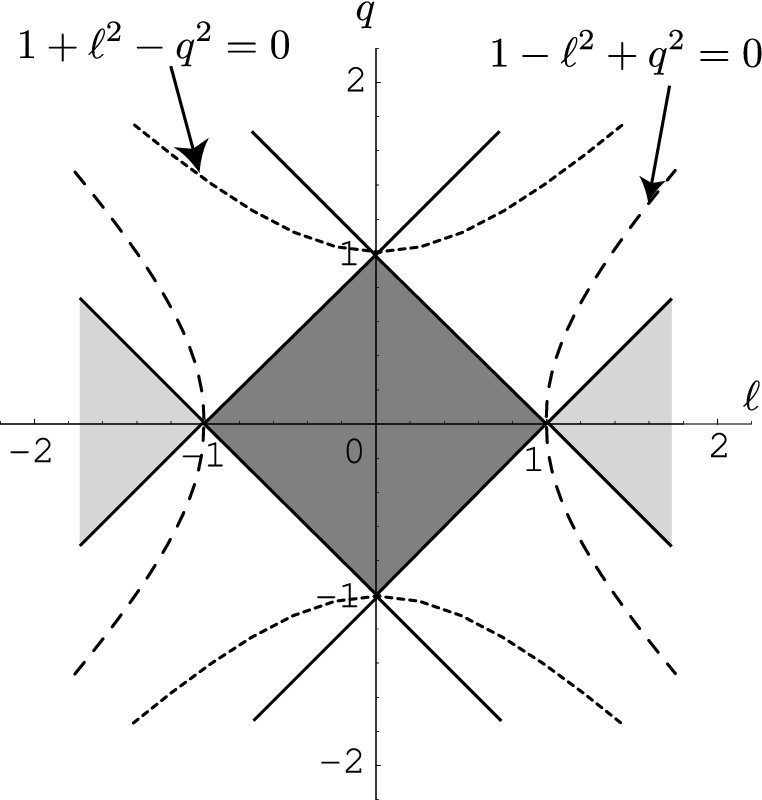
We see that $\rho$ is bounded as $\rho_{min}\leq\rho\leq\rho_{max}$ because the right hand side of (36) should be positive, where

		$\displaystyle\rho_{min}^{2}=\frac{1}{2\Omega^{2}}\left(1+\ell^{2}-q^{2}-\sqrt{(1+\ell+q)(1+\ell-q)(1-\ell+q)(1-\ell-q)}\right),$		(37)
		$\displaystyle\rho_{max}^{2}=\frac{1}{2\Omega^{2}}\left(1+\ell^{2}-q^{2}+\sqrt{(1+\ell+q)(1+\ell-q)(1-\ell+q)(1-\ell-q)}\right),$		(37)

with

		$\displaystyle 1+\ell^{2}-q^{2}\geq 0,$		(38)
		$\displaystyle(1+\ell+q)(1+\ell-q)(1-\ell+q)(1-\ell-q)\geq 0.$		(38)

Allowed region of the parameters are shown in Fig.1.

If $q\neq 0$ , it is easy to show that

\displaystyle(1-\Omega^{2}\rho_{min}^{2})(1-\Omega^{2}\rho_{max}^{2})>0.

(39)

It means that there are two cases:

	$\displaystyle\mbox{(i)}$	$\displaystyle(1-\Omega^{2}\rho_{min}^{2})>0\quad\mbox{and}\quad(1-\Omega^{2}\rho_{max}^{2})>0\quad$	$\displaystyle\mbox{for}$	$\displaystyle 1-\ell^{2}+q^{2}>0,$		(40)
	$\displaystyle\mbox{(ii)}$	$\displaystyle(1-\Omega^{2}\rho_{min}^{2})<0\quad\mbox{and}\quad(1-\Omega^{2}\rho_{max}^{2})<0\quad$	$\displaystyle\mbox{for}$	$\displaystyle 1-\ell^{2}+q^{2}<0.$		(40)

In the first case, the Killing vector field $\xi$ is timelike everywhere on the world surface $\Sigma$ , while $\xi$ is spacelike everywhere on $\Sigma$ in the second case. In the both cases (i) and (ii), the strings are rigidly rotating[13]. The solutions in the case (i) give the stationary rotating strings.

Refer to caption — Figure 1: Parameter regions. The shaded areas are the parameter regions for the rigidly rotating strings, the cases (i) and (ii). The dark shaded area is the parameter region for the stationary rotating strings, the case (i).

There are three singularities of $h^{red}_{AB}$ given by (32), $\rho=0$ , $\rho=\rho_{q}:=\sqrt{1-q^{2}}/|\Omega|$ and $\rho=1/|\Omega|$ . For the stationary string, $0\leq\rho\leq\rho_{max}\leq\rho_{q}$ . The point $\rho=0$ is a fixed point of the rotational isometry generated by the Killing vector $\partial/\partial\varphi$ . When $q\neq 0$ the point $\rho=\rho_{q}$ is also a fixed point of the rotation, that is, there are two centers in this space. When $q=0$ the point $\rho=\rho_{q}$ becomes a circle.

The scalar curvature of the metric (32) is calculated as

\displaystyle R=\frac{-6q^{4}+2\left(\Omega^{2}\rho^{2}+4\right)\left(1-\Omega^{2}\rho^{2}\right)q^{2}-2\left(1-\Omega^{2}\rho^{2}\right)^{3}}{\left(1-\Omega^{2}\rho^{2}\right)^{2}\left(1-q^{2}-\Omega^{2}\rho^{2}\right)^{3}}.

(41)

One of the centers $\rho=\rho_{q}$ is the curvature singularity, while the other center $\rho=0$ is regular point. The scalar curvature vanishes at $\rho=0$ when $q^{2}=1/3$ . When $q^{2}>1/3$ , the scalar curvature is positive everywhere, while the curvature becomes negative near $\rho=0$ when $q^{2}<1/3$ . When $q$ is small enough, the scalar curvature has the minimum point near $\rho=\rho_{q}$ . Fig.2 shows the scalar curvature as the function of $|\Omega|\rho$ .

III Solutions for Stationary Rotating Strings

If we choose the function $N_{(2)}$ as

\displaystyle N_{(2)}=1-q^{2}-\Omega^{2}\rho^{2},

(42)

two first order differential equations (35) and (36) become

		$\displaystyle\varphi^{\prime}=\frac{\ell}{\|\Omega\|}\frac{1-\Omega^{2}\rho^{2}}{\rho^{2}},$		(43)
		$\displaystyle{\rho}^{\prime 2}=(1-q^{2}-\Omega^{2}\rho^{2})-\frac{\ell^{2}(1-\Omega^{2}\rho^{2})}{\Omega^{2}{\rho}^{2}}.$		(44)

We also see that (30) with (33) simply gives

\displaystyle z=q\sigma.

(45)

The change of signature of parameters:

\displaystyle\ell\to-\ell,\quad q\to-q,\quad\mbox{and}\quad\Omega\to-\Omega,

(46)

can be absorbed by the inversion of coordinates:

\displaystyle\varphi\to-\varphi,\quad z\to-z,\quad\mbox{and}\quad t\to-t,

(47)

respectively. Then we restrict ourselves in the case $\ell\geq 0,q\geq 0$ and $\Omega\geq 0$ .

III.1 Limiting cases

Before we obtain general solutions for the stationary rotating strings, we see that two limiting cases of parameters $\ell,q$ , (1) $\ell+q=1$ and (2) $\ell=0$ (see Figs.3 and 4).

III.1.1 Helical strings

In the case of $\ell+q=1$ , we find from (37) that $\rho$ should take a constant value $\rho_{0}$ , where

\displaystyle\rho_{0}=\rho_{max}=\rho_{min}=\frac{\sqrt{\ell}}{\Omega}.

(48)

When $q\neq 0$ , using (43) and (45) we see that solutions are described by

\displaystyle\rho=\rho_{0},\quad

\displaystyle\varphi=\Omega z.

(49)

We call these solutions a helical strings. The shapes of helical strings are shown in Fig.3. In the limit $\ell=0$ i.e., $q=1$ , the solutions reduce to the straight string solution.

We can calculate the proper length of snapshot of the string with respect to the metric (12) as

\displaystyle\int ds=\int\sqrt{(1-\Omega^{2}\rho^{2})d\rho^{2}+\rho^{2}d\varphi^{2}+(1-\Omega^{2}\rho^{2})dz^{2}}.

(50)

For the helical strings (49), the proper length for $z$ -interval $z\sim z+\Delta z$ is given by

\displaystyle\int\sqrt{\rho_{0}^{2}d\varphi^{2}+(1-\Omega^{2}\rho_{0}^{2})dz^{2}}=\int_{z}^{z+\Delta z}dz=\Delta z.

(51)

It shows that all helical strings have the same proper length as the straight string with the same $z$ -interval.

In the inertial reference frame (5), the helical strings are described by

		$\displaystyle\bar{\rho}=\rho_{0},$		(52)
		$\displaystyle\bar{\varphi}=\Omega(\bar{z}+\bar{t}).$		(52)

The solutions consist of a down-moving wave of the angular frequency $\Omega$ and the amplitude $\rho_{0}$ given by (48) with the circular polarization. The pitch of helix, equivalently the wave length, is given by $2\pi\Omega^{-1}$ . The two-dimensional world surface of helical string has another Killing vector $\partial_{\bar{z}}+\Omega\partial_{\bar{\varphi}}$ which is tangent to it in addition to $\partial_{\bar{t}}+\Omega\partial_{\bar{\varphi}}$ . It means the world surface of helical string is a homogeneous space.

III.1.2 Planar strings

In the case of $\ell=0$ , it is convenient to use the rigidly rotating Cartesian coordinate

\displaystyle x=\rho\cos\varphi,\quad y=\rho\sin\varphi.

(53)

From (43) we can set $\varphi=0$ ( $y=0$ ) without loss of generality. Then, from (44) and (36) we have

\displaystyle q^{2}\left(\frac{dx}{dz}\right)^{2}=1-q^{2}-\Omega^{2}x^{2}.

(54)

The strings are confined in $x-z$ plane, so we call these planer strings. The solutions for (54) are

\displaystyle x=\rho_{max}\sin\left(\frac{\Omega z}{q}\right),

(55)

where the amplitude of the waving string $\rho_{max}$ is given by the parameters $\Omega$ and $q$ as

\rho_{max}=\frac{\sqrt{1-q^{2}}}{\Omega}.

The shape of planer strings is depicted in Fig.4.

In the inertial Cartesian coordinate, the planar strings are described by

	$\displaystyle\bar{x}=\rho_{max}\sin\left(\frac{\Omega\bar{z}}{q}\right)\cos\Omega\bar{t},$		(56)
	$\displaystyle\bar{y}=\rho_{max}\sin\left(\frac{\Omega\bar{z}}{q}\right)\sin\Omega\bar{t}.$		(56)

These strings consist of a standing wave which is superposition of an up-moving wave and a down-moving wave in the equal amplitude. In the limit $q=1$ the solution becomes the straight string solution.

III.1.3 General cases

In general, when $\ell\neq 0$ , two first order differential equations (43) and (44) are integrated in the form

		$\displaystyle{\rho}^{2}=\frac{1}{2}\left\{(\rho_{max}^{2}+\rho_{min}^{2})-(\rho_{max}^{2}-\rho_{min}^{2})\cos\left(2\Omega\sigma\right)\right\},$		(57)
		$\displaystyle\frac{2\ell}{\Omega^{2}}\tan\left({\varphi}-\varphi_{0}+\ell\Omega\sigma\right)=(\rho_{max}^{2}+\rho_{min}^{2})\tan\left(\Omega\sigma+\frac{\pi}{4}\right)-(\rho_{max}^{2}-\rho_{min}^{2}),$		(58)

where $\varphi_{0}$ is a constant. (see also ref[11].)

In the case of $q=0$ , (45) leads that strings are confined in a $z=const.$ plane ( $x-y$ plane). In this case, the stationarity of the strings breaks down at the light cylinder $\rho=\rho_{max}=1/\Omega$ . Since the point $\rho=1/\Omega$ is curvature singularity, the geodesics have end points there. This case is a special case of Burden’s solution[16] and discussed in detail by Frolov et al[13]. The shape of strings in $x-y$ plane is shown in Fig.5.

Both of the functions $\rho(\sigma)$ and $\varphi(\sigma)$ in the solution (57) and (58) are periodic with respect to $\sigma$ , but the periods are different. It is clear that

\displaystyle\rho(\sigma+\sigma_{p})=\rho(\sigma),

(59)

where $\sigma_{p}=\pi/\Omega$ . In this period of $\sigma$ , $\varphi$ varies as

\displaystyle{\varphi}(\sigma+\sigma_{p})={\varphi}(\sigma)+\pi(1-\ell).

(60)

Suppose that $\ell$ is a rational number which can be expressed as $\ell=a/b$ , where $a$ and $b$ are relatively prime. During $\sigma$ increases by $n$ times $\sigma_{p}$ , $\varphi$ varies as

	$\displaystyle{\varphi}(\sigma+n\sigma_{p})$	$\displaystyle={\varphi}(\sigma)+n\pi(1-\ell)$		(61)
		$\displaystyle={\varphi}(\sigma)+n\frac{b-a}{b}\pi.$		(62)

If the second term in the right hand side holds

\displaystyle n\frac{b-a}{b}\pi=2\pi m,\quad(n,m:\mbox{natural numbers})

(63)

$\rho$ and $\varphi$ have a common period. The least value of $n$ , say $n_{\ell}$ , is determined by

\displaystyle n_{\ell}

\displaystyle=\frac{2b}{\mathrm{GCD}\bigr[2b,(b-a)\bigr]},

(64)

where $\mathrm{GCD}\left[x,y\right]$ is the greatest common divisor of $x,y$ . The projected curve in the reduced two-dimensional space is closed if $\ell$ is rational. The closed curve consists of $n_{\ell}$ elements; each element starts off $\rho_{max}$ , evolves through $\rho_{min}$ , and ends at $\rho_{max}$ . Till the curve returns to its starting point, $\varphi$ laps $2\pi m_{\ell}$ , i.e., the curve wraps around the rotation axis $m_{\ell}$ times, where $m_{\ell}$ is given by

\displaystyle\ m_{\ell}=\frac{1-\ell}{2}n_{\ell}.

(65)

Suppose a closed geodesic in the reduced two-dimensional space which consists $n$ elements and which wraps around the rotation axis $m$ times. The parameter $\ell$ for this string is given by

\displaystyle\ell=1-\frac{2m}{n}.

(66)

When $\ell$ is irrational number, the two-dimensional geodesic is not closed.

The strings with rational $\ell$ have periodic structure in $z$ with the period $Z_{p}=n_{\ell}q\sigma_{p}=\pi n_{\ell}q/\Omega$ . On the other hand, the strings with irrational $\ell$ have no periodicity. We show the shapes of strings in Figs. 6 for $\ell=1/5$ , $1/3$ , and $1/2$ .

IV Energy, Momentum and Angular Momentum

By varying the action (1) by $g_{\mu\nu}$ we see that the string energy-momentum tensor $T^{\mu\nu}$ is given by

	$\displaystyle\sqrt{-g}T^{\mu\nu}(x^{\lambda})$	$\displaystyle=-\mu\int d^{2}\zeta\Theta^{\mu\nu}(\zeta^{c})\delta^{(4)}\left(x^{\lambda}-x^{\lambda}(\zeta^{c})\right),$		(67)
		$\displaystyle\Theta^{\mu\nu}=\sqrt{-\gamma}\gamma^{ab}\partial_{a}x^{\mu}\partial_{b}x^{\nu},$		(68)

where $x^{\lambda}(\zeta^{c})$ is the solution of $\Sigma$ .

In the inertial reference system (5), we can rewrite the energy-momentum tenser for the stationary rotating strings as

\displaystyle\sqrt{-g}T^{\bar{\mu}\bar{\nu}}(\bar{t},\bar{\rho},\bar{\varphi},\bar{z})=-\mu\int d\tau d\sigma\ \Theta^{\bar{\mu}\bar{\nu}}(\sigma)\ \delta\left(\bar{t}-\tau\right)\delta\left(\bar{\rho}-\bar{\rho}(\sigma)\right)\delta\left(\bar{\varphi}-\bar{\varphi}(\tau,\sigma)\right)\delta\left(\bar{z}-\bar{z}(\sigma)\right).

(69)

From (43), (45) and (36), we obtain $\Theta^{\bar{\mu}\bar{\nu}}$ explicitly. (See Appendix B.)

Now, we define the string energy, $E$ , the angular momentum, $J$ , and the momentum along the rotating axis, $P$ . We consider infinitely long strings with periodic structure, i.e., $\ell$ is assumed to be a rational number, then we define $E,J$ and $P$ for one period, $\bar{z}\sim\bar{z}+Z_{p}$ as

$\displaystyle E$	$\displaystyle:=\int_{\rho_{min}}^{\rho_{max}}d\bar{\rho}\int_{0}^{2\pi}d\bar{\varphi}\int_{0}^{Z_{p}}d\bar{z}\sqrt{-g}~T^{\bar{t}}_{\ \bar{\nu}}(-\partial_{\bar{t}})^{\bar{\nu}}=\mu\int_{0}^{n_{l}\sigma_{p}}d\sigma\ \Theta^{\bar{t}}_{~{\bar{t}}}(\sigma),$	(70)
$\displaystyle J$	$\displaystyle:=\int_{\rho_{min}}^{\rho_{max}}d\bar{\rho}\int_{0}^{2\pi}d\bar{\varphi}\int_{0}^{Z_{p}}d\bar{z}\sqrt{-g}~T^{\bar{t}}_{\ \bar{\nu}}(\partial_{\bar{\varphi}})^{\bar{\nu}}=-\mu\int_{0}^{n_{l}\sigma_{p}}d\sigma\ \Theta^{\bar{t}}_{~{\bar{\varphi}}}(\sigma),$	(71)
$\displaystyle P$	$\displaystyle:=\int_{\rho_{min}}^{\rho_{max}}d\bar{\rho}\int_{0}^{2\pi}d\bar{\varphi}\int_{0}^{Z_{p}}d\bar{z}\sqrt{-g}~T^{\bar{t}}_{\ \bar{\nu}}(\partial_{\bar{z}})^{\bar{\nu}}=-\mu\int_{0}^{n_{l}\sigma_{p}}d\sigma\ \Theta^{\bar{t}}_{~\bar{z}}(\sigma).$	(72)

It is easy to calculate these quantities as

$\displaystyle E$	$\displaystyle=\frac{\pi\mu}{\|\Omega\|}n_{\ell}(1-\ell^{2}),$	(73)
$\displaystyle J$	$\displaystyle=\frac{\pi\mu}{2\Omega\|\Omega\|}n_{\ell}(1-\ell^{2}-q^{2}),$	(74)
$\displaystyle P$	$\displaystyle=-\frac{\pi\mu}{\Omega}n_{\ell}\ell q.$	(75)

We can also define the averaged values of theses quantities per unit length of $z$ as

$\displaystyle\mathinner{\langle{E}\rangle}$	$\displaystyle:=E/Z_{p}=\mu\frac{1-\ell^{2}}{\|q\|},$	(76)
$\displaystyle\mathinner{\langle{J}\rangle}$	$\displaystyle:=J/Z_{p}=\frac{\mu}{\Omega}\frac{1-\ell^{2}-q^{2}}{2\|q\|},$	(77)
$\displaystyle\mathinner{\langle{P}\rangle}$	$\displaystyle:=P/Z_{p}=-\mu\ell\mathrm{sign}(\Omega q).$	(78)

These quantities are applicable for the strings with irrational $\ell$ .

When $\ell\neq 0$ and $q\neq 0$ , we see $P\neq 0$ , that is, the strings move along the rotating axis. Although the rotating velocity of a string segment is perpendicular to the rotation axis, the physical velocity of the Nambu-Goto string is orthogonal to the segment. Since the strings with $\ell\neq 0$ and $q\neq 0$ have inclination to the rotation axis, then the physical velocity of string segments have the component along the rotation axis. This is the reason for non-vanishing $P$ . In the planar string case, $\ell=0$ , the rotating velocity is physical, that is, the velocity is orthogonal to the string because the planar string is confined in $x-z$ plane. Then the planar string does not move along the rotation axis. It is consistent with the fact that the planar string consists of a standing wave as mentioned before.

In order to see the effective equation of state[2] for the stationary rotating strings, we transform the reference system such that the averaged value of momentum $\mathinner{\langle{P}\rangle}$ vanishes. Using the fact that

\displaystyle\mathinner{\langle{T^{\bar{t}\bar{t}}-T^{\bar{z}\bar{z}}}\rangle}~\mbox{and}~\mathinner{\langle{T^{\bar{t}\bar{t}}T^{\bar{z}\bar{z}}-(T^{\bar{t}\bar{z}})^{2}}\rangle}

(79)

are invariant under the Lorentz transformation along the $\bar{z}$ -axis, we obtain effective line density, $\tilde{\mu}$ , and effective tension, $\tilde{\cal T}$ , as

		$\displaystyle\tilde{\mu}=\frac{\mu}{2\|q\|}\left[{1-\ell^{2}+q^{2}}+\sqrt{(1-q-\ell)(1-q+\ell)(1+q-\ell)(1+q+\ell)}\right],$		(80)
		$\displaystyle\tilde{\cal T}=\frac{\mu}{2\|q\|}\left[{1-\ell^{2}+q^{2}}-\sqrt{(1-q-\ell)(1-q+\ell)(1+q-\ell)(1+q+\ell)}\right].$		(80)

In general, it holds that $\tilde{\mu}\tilde{\cal T}=\mu^{2}$ and $\tilde{\mu}\geq\tilde{\cal T}$ . In the case of helical strings, there exists no inertial reference system such that $\mathinner{\langle{P}\rangle}$ vanishes because a single wave moves with the velocity of light along the rotating axis.

V Conclusion

We study stationary rotating Nambu-Goto strings in Minkowski spacetime. It has been shown that the stationary rotating strings with an angular velocity $\Omega$ are described by geodesics in two-dimensional curved spaces with positive definite metrics with a parameter, $q$ in this paper. The metrics admit a Killing vector which generates rotation symmetry, then the geodesics in the two-dimensional spaces have a constant of motion, $\ell$ in this paper. Therefore, the stationary rotating strings in Minkowski spacetime are characterized by three parameters $(\Omega,q,\ell)$ .

One of the typical stationary rotating strings are the ‘helical strings’, $|q|+|\ell|=1$ , where a snapshot looks a helix. The world surface of the helical string is the two-dimensional homogeneous space embedded in Minkowski spacetime. For general $(\Omega,q,\ell)$ , stationary rotating strings have quasi-periodic structure along the rotation axis. Only in the case of rational $\ell$ , the strings have exact periodicity. The strings display much variation in the shape which depends on $q$ and $\ell$ .

We have obtained the following averaged values per unit length along the rotation axis: energy, angular momentum and linear momentum along the axis. It should be noted that the rotation of the strings around the axis induces the linear momentum along the axis because of the inclination of string segments.

By the advantage of the analytic solutions of the string motion, we can calculate the energy-momentum tensor easily. Then, we can study the gravitational field yielded by the stationary rotating strings, especially gravitational wave emission. It is important to clarify the property of the gravitational waves from the stationary rotating strings for verification of their existence in the universe. We will report this issue in near future[17].

It is also interesting problem to construct all cohomogeneity-one string in Minkowski[15, 18], de Sitter, and anti-de Sitter[19] spacetimes. Furthermore, it would be challenging work to find the general solutions of stationary rotating strings in the black hole spacetimes as an extended work of ref.[13].

Acknowledgments

We would like to thank K. Nakao and C.-M. Yoo for useful discussions. HN is supported by a JSPS Research Fellowship for Young Scientists, No. 5919. He is also supported by JSPS for Research Abroad and in part by the NSF through grants PHY-0722315, PHY-0701566, PHY-0714388, and PHY-0722703, and from grant NASA 07-ATFP07-0158.

Appendix A Potential in Two-dimensions

We consider a particle in the two-dimensional flat space driven by a potential force. In general, every metric of two-dimensional space is written in conformal flat form. The metric (32) is written in the form

	$\displaystyle ds_{red}^{2}$	$\displaystyle=(1-q^{2}-\Omega^{2}\rho^{2})\left(d\rho^{2}+\frac{\rho^{2}}{1-\Omega^{2}\rho^{2}}d\tilde{\varphi}^{2}\right)$		(81)
		$\displaystyle=F(x^{A})\left(dr^{2}+r^{2}d\varphi^{2}\right),$		(81)

where

		$\displaystyle F=\frac{1-q^{2}-\Omega^{2}\rho^{2}}{1-\Omega^{2}\rho^{2}}(1+\sqrt{1-\Omega^{2}\rho^{2}})^{2}e^{-2\sqrt{1-\Omega^{2}\rho^{2}}},$		(82)
		$\displaystyle r=\frac{\rho}{1+\sqrt{1-\Omega^{2}\rho^{2}}}e^{\sqrt{1-\Omega^{2}\rho^{2}}}.$		(82)

Using the argument from (22) to (29) inversely, we see that geodesics in the metric (81) is equivalent to the orbits of the particle whose dynamics is governed by the action

\displaystyle S=\int\left[p_{A}{x}^{\prime A}-N_{(2)}{\cal H}\right]d\sigma

(83)

References

- [1] T. W. B. Kibble, J. Phys. A9, 1387 (1976).
- [2] A. Vilenkin and E. P. S. Shellard, Cosmic Strings and Other Topological Defects (Cambridge University Press, 1994).
- [3] E. P. S. Shellard, Nucl. Phys. B 283, 624 (1987).
- [4] A. Albrecht and N. Turok, Phys. Rev. D 40, 973 (1989).
- [5] D. P. Bennett and F. R. Bouchet, Phys. Rev. D 41, 2408 (1990).
- [6] B. Allen and E. P. S. Shellard, Phys. Rev. Lett. 64, 119 (1990).
- [7] S. Sarangi and S. H. H. Tye, Phys. Lett. B 536, 185 (2002).
- [8] G. Dvali and A. Vilenkin, JCAP 0403, 010 (2004)
- [9] E. J. Copeland, R. C. Myers and J. Polchinski, JHEP 0406, 013 (2004).
- [10] M. G. Jackson, N. T. Jones and J. Polchinski, JHEP 0510, 013 (2005).
- [11]
C. J. Burden and L. J. Tassie, Aust. J. Phys., 35 (1982), 223;
C. J. Burden and L. J. Tassie, Aust. J. Phys. 37 (1984), 1. - [12]
H.J. de Vega, A.L. Larsen, and N. Sanchez, Nucl. Phys.B427, 643 (1994);
A.L. Larsen and N. Sanchez, Phys. Rev. D50, 7493 (1994);
A.L. Larsen and N. Sanchez, Phys. Rev. D51, 6929 (1995);
H.J. de Vega and I.L. Egusquiza, Rev. D54, 7513 (1996). - [13]
V. P. Frolov, V. Skarzhinsky, A. Zelnikov and O. Heinrich,
Phys. Lett. B 224, 255 (1989);
V. P. Frolov, S. Hendy and J. P. De Villiers, Class. Quant. Grav. 14, 1099 (1997). - [14] M. R. Anderson, ”The Mathematical Theory of Cosmic Strings”, Institute of Physics Publishing (2003),
- [15] H. Ishihara and H. Kozaki, Phys. Rev. D 72, 061701 (2005).
- [16] C. J. Burden, Phys. Lett. 164B, 277 (1985).
- [17] K. Ogawa, H. Ishihara, H. Kozaki, and H. Nakano in preparation.
- [18] H. Kozaki, T.Koike, and H. Ishihara, in preparation.
- [19] T.Koike, H. Kozaki, and H. Ishihara, Phys. Rev. D 77, 125003 (2008).