Learning Sequences

The fringe of any state $S$ in a learning space is defined to be the set of concepts that, when added to or removed from $S$, lead to another state in the learning space. Fringes are important to ALEKS because they describe the concepts that the assessed student is most ready to learn, or has the most shaky learning of. We may distinguish the outer fringe of concepts a student is ready to learn, those concepts $x$ such that $S\cup\{x\}$ is also a state in the learning space, from the inner fringe of concepts that a student may have most recently learned, those concepts $x$ such that $S\setminus\{x\}$ is also a state. The fringe is the union of the outer and inner fringes. In a learning space (or more generally, in any medium) each state may be uniquely identified by the pair of its outer and inner fringes.

In a quasi-ordinal space, the inner fringe of $S$ consists of the maximal concepts in $S$, and the outer fringe consists of the minimal concepts not in $S$. The fringe of $S$ may be calculated easily in a single pass through the edges $x\rightarrow y$ of the Hasse diagram: if $x\rightarrow y$ and $x\notin S$, then $y$ cannot be in the fringe, and if $x\rightarrow y$ and $y$ in $S$, then $x$ cannot be in the fringe. We initialize a set $F$ to consist of the whole domain, and remove $x$ or $y$ from $F$ whenever we discover a covering relation that prevents it from belonging to the fringe; the remaining set at the end of this scan is the fringe.

To determine the likelihood that a student knows each concept in a learning space, from a given set of results on asked questions, ALEKS uses an algorithm based on listing all states in the learning space. The algorithm used by ALEKS can be explained most easily in terms of reverse search (Avis and Fukuda, 1996), a general technique for developing generation algorithms for many types of combinatorial structures.

Suppose we have chosen a topological ordering (also known as a linear extension) of the concepts in a partial order; that is, a sequence of the concepts such that, if $x<y$ in the order, then $x$ must appear prior to $y$ in the sequence. For instance, one may sort the concepts by the length of the longest path leading to each concept in the Hasse diagram, with ties broken arbitrarily among concepts having paths of the same length; the resulting sorted sequence is a topological ordering. Then, given any state $S$ in the knowledge space, one may find another state $S\setminus\{x\}$ where $x$ is chosen to be the concept belonging to $S$ that has the latest position in the topological ordering. We call $S\setminus\{x\}$ the predecessor of $S$. In this way, we disambiguate the accessibility property of learning spaces and make a concrete choice of which concept to remove to form the predecessor of any state. If we repeat this removal process, starting from any state, we will eventually reach the empty set, so the graph formed by connecting each state to its predecessor is a tree, rooted at the empty set. Reverse search, applied to this predecessor relationship, amounts to performing a depth first traversal of this tree.

To be more specific, we perform a recursive traversal of the tree defined above, maintaining as we do for each state $S$ a set ${\rm children}(S)$ of the concepts that may be added to $S$ to form another state that is a child of $S$ in the predecessor tree. Then, when the recursion steps from $S$ to $S\cup\{x\}$, we calculate ${\rm children}(S\cup\{x\})$ from ${\rm children}(S)$ by removing from ${\rm children}(S)$ any $y$ occurring prior to $x$ in the topological order, and adding to ${\rm children}(S)$ any concept $y$ reachable from $x$ by a Hasse diagram edge $x\rightarrow y$ such that all other prererequisites of $y$ already belong to $S$. Once we have calculated ${\rm children}(S\cup\{x\})$, we may output $S\cup\{x\}$ as one of our states and continue recursively to each state $S\cup\{x,y\}$ for each $y$ in ${\rm children}(S\cup\{x\})$, and so on.

Very little is needed in the way of data structures beyond the Hasse diagram itself to implement this recursive traversal efficiently. Primarily, we need a way of quickly determining whether all prerequisites of some concept $y$ belong to the set $S$ we are traversing. This may be done efficiently by maintaining, for each $y$, a count of the prerequisites of $y$ that do not yet belong to $S$, decrementing that count for each successor of $x$ whenever we step from $S$ to $S\cup\{x\}$, and incrementing the count again when our recursive traversal returns from $S\cup\{x\}$ to $S$. In this way we may test prerequisites in constant time, and use time proportional to the number of Hasse diagram edges out of $x$ to update counts whenever we step from state to state. Alternatively, the method used within the 2006 implementation of ALEKS is to store a bitmap representation of $S$, and mask it against a bitmap representing the predecessors of $y$ whenever such tests are needed; theoretically this method requires time proportional to the number of items in the learning space per test, but in practice it is fast because typical modern computer architectures allow for the testing of prerequisite relations for 32 concepts simultaneously in a single machine instruction.

The total time spent copying lists of children in this procedure can be charged using amortized time analysis against the time to generate each child state. Therefore, the bottleneck for time analysis of the procedure is the part of the time spent testing successors of $x$ and testing whether to add those successors to ${\rm children}(S\cup\{x\})$. As described above, each such test can be implemented in linear time, so the total time for the algorithm is proportional to the sum, over all states in the learning space, of the number of Hasse diagram edges that are outgoing from the last concept in each state. In typical examples the Hasse diagrams are relatively sparse and the time per state may approach a constant, but even in the worst case (Figure 2) the time is no more than $O(n)$ per state in a learning space with $n$ concepts. It is this level of state generation efficiency that we hope to approach or meet with our more general learning space representation.

While a student is being assessed, he or she will have answered some of the assessment questions correctly and some incorrectly. We desire to infer from these results likelihoods that the student understands each of the concepts in the knowledge space, even those concepts not explicitly tested in the assessment.

The inference method used by ALEKS (Falmagne and Doignon, 1988; Falmagne et al., 1990) applies more generally to any system of sets, and can be interpreted using Bayesian probability methods. We begin with a prior probability distribution on the feasible states of the learning space. In the most simple case, we can assume an uninformative uniform prior in which each state is equally likely, but the method allows us to incorporate prior probabilities based on any easily computable function of the state, such as the number of concepts in the set represented by the state. These prior probilities may incorporate knowledge about the student’s age or grades, or results from assessments in previous sessions that the student may have had with ALEKS; for instance, if a previous session assessed the student as being in a certain state, we could use an a priori probability distribution based on distance from that state in our next assessment. However, in the 2006 implementation of ALEKS only uniform prior probabilities are used.

We also assume a conditional probability that the student, in a given state, will answer a question correctly or incorrectly: if the question tests a concept within the set represented by the state, we assume a high probability of a correct answer, while if a question tests a concept not within the set represented by the state, we assume a low probability of a correct answers. Answers opposite to what the given state predicts can be ascribed to careless mistakes or lucky guesses, and we assume that incidences of such answers are independent of each other. ALEKS’ test questions are designed so that lucky guesses are very rare; therefore, the necessity for accurate assessment in the presence of careless mistakes is of much greater significance to the design of the assessment procedure, but this also means that it is necessary to ascribe different rates to these two types of events. With these assumptions, we may use Bayes’ rule to calculate posterior probabilities of each state. To do so, we calculate for each state a likelihood, the product of its prior probability with a set of terms, one term per already-asked assessment question. The value of each term depends on whether the student answered the question correctly and whether the concept tested by the question belongs to the given state. Once we have calculated these likelihoods for all states, they may be converted to probabilities by dividing them all by a common constant of proportionality, the sum of the likelihoods of all states.

From these posterior probabilities of states we wish to calculate posterior probabilities of individual concepts. To do so, we sum the probabilities of all states containing a given concept. ALEKS’s assessment procedure calculates the probabilities of all concepts in this way, and then chooses to test the student on the most informative concept: the one with probability closest to 50% of being known. Eventually, all concepts will have probabilities bounded well away from 50%, at which point the evaluation procedure terminates.

Although described above as a separate sum for each concept, ALEKS implements this probability calculation via a single pass through the states of the learning space. When the state generation procedure steps from a state $S$ to a child state $S\cup\{x\}$, it calculates the likelihood (product of terms for each answered question) from the new state by multiplying the old likelihood by a single term for the questions based on concept $x$. It totals the likelihood of all states descending from $S\cup\{x\}$ in the recursive search, and adds this total likelihood to that of concept $x$. Then, when returning from $S\cup\{x\}$ to $S$, it adds the total likelihood calculated for $S\cup\{x\}$ into that for $S$. In this way, the likelihood for each concept is calculated in constant time per state, and the constant of proportionality needed to turn these likelihoods into probabilities is calculated as the total likelihood at the root of the recursion.

If $x<y$ in the partial order defining the system’s learning space, $x$ will be assessed as having higher probability than $y$ of being known; therefore, the set of concepts returned by this assessment algorithm is guaranteed to be a feasible knowledge state for the given quasi-ordinal space.

Although the assessment procedure described above works well for partial orders of 50 to 100 concepts, it becomes too slow for larger learning spaces due to the need for the algorithm to list all states in the space and the combinatorial explosion in the number of states generated for those spaces. Therefore, the ALEKS system resorts to a sampling scheme that allows its assessment procedure to run at interactive speeds for much larger learning spaces. This sampling scheme is based on three concepts, all depending on the details of the definition of the learning space in terms of partial orders: distance between concepts, definition of smaller learning spaces from sampled concepts, and bounding concept likelihoods from their prerequisites and postrequisites.

To generate smaller samples of the set of concepts used to define a learning space, ALEKS uses a notion of distance between two concepts in a partial order. To define the distance between $x$ and $y$, define $\Delta_{x,y}$ to be the set of items whose comparison to $x$ is different from its comparison to $y$. That is,

Then the distance $d(x,y)$ between $x$ and $y$ is defined to be $|\Delta_{x,y}|-1$. This distance satisfies the mathematical axioms defining a metric space: $d(x,x)=0$, $d(x,y)=d(y,x)$. For any $x$, $y$, and $z$, $\Delta_{x,z}\subset\Delta_{x,y}\cup\Delta_{y,z}$, and the union is not disjoint as $y$ belongs to both sides, so $d(x,z)\leq d(x,y)+d(y,z)$.

ALEKS then chooses a suitable distance threshhold $\delta$, and a sample $S$ of the concepts of the learning space such that every concept is within distance $\delta$ of a member of $S$. Although there is no mathematical proof of such a fact, the intent of this sampling technique is that assessment on a nearby sample concept is likely to be informative about the assessment of each unsampled concept.

Once a sample of concepts has been chosen, ALEKS must form a learning space describing the knowledge states possible for that sample, so that it can apply its assessment procedure to the sample. For quasi-ordinal learning spaces, this process of forming a learning space on the sample is very simple: one need merely restrict the given partial order defining the space to the sampled concepts, and build a learning space from the restricted order (Figure 3).

Finally, the assessment of likelihoods on the sampled concepts is used to bound the likelihoods of the remaining unsampled concepts, to determine which ones the student is likely to know or not to know. If $x<y$, $y$ belongs to the sample, and the student knows $y$ with probability $p$, then the student is taken to know the easier concept $x$ with probability at least $p$. Similarly, if $x<y$, $x$ belongs to the sample, and the student knows $x$ with probability $p$, then the student is taken to know the harder concept $y$ with probability at most $p$. However, there is something of a mismatch between these likelihood bounds and the distance-based sampling procedure: it is possible for the nearby samples to an unsampled concept $x$ to all be incomparable to $x$, in which case we cannot find any useful bounds for the likelihood of $x$.

This sampling process, sample learning space construction, and likelihood bound, are used together repeatedly to refine the portion of the learning space that is relevant for the student. Initially, all states are considered relevant, and a sample with a high distance threshhold is chosen. After several steps of refinement, a larger number of concepts have likelihoods that can be bounded away to one side or another of 50%, and a sample is chosen with a smaller distance threshhold among only those remaining informative concepts. Eventually, this refinement process converges with all concepts having likelihoods bounded away from 50%, which we may use to construct a most likely knowledge state for the student.

For learning spaces not defined from partial orders, we may have to replace these constructions with alternative techniques. However, it will still be necessary to have some way of sampling the concepts of the learning space, building a smaller learning space from the sample, and using assessments on the sample to bound likelihoods of unsampled concepts, because this sampling procedure is crucial to limiting the number of states generated in the assessment procedure and thereby keeping the assessment calculation’s times fast enough for human interaction.

Given any learning space, there may be many orderings through which a student, starting from no knowledge, could learn all the concepts in the space. We call such an ordering a learning sequence; in the combinatorics literature these are also known as basic words. Formally, a learning sequence $\sigma$ can be defined as a one-to-one map from the integers $\{0,1,2,\ldots n-1\}$ to the $n$ concepts forming the domain of a learning space, with the property that each prefix $P_{i}(\sigma)=\sigma(\{0,1,2,\ldots i-1\})$ is a valid knowledge state in the learning space. The sequence of prefixes $P_{0}(\sigma),P_{1}(\sigma),\ldots P_{n-1}(\sigma)$ forms a shortest path in the learning space from the empty set to the whole domain, and for any such path the sequence of items by which one state in the path differs from the next forms a learning sequence.

For instance, in the learning space depicted in Figure 1, the leftmost path from the bottom state (the empty set) to the top set (the whole domain) passes through the sequence of states $\emptyset$, $\{A\}$, $\{A,C\}$, $\{A,C,E\}$, $\{A,B,C,E\}$, $\{A,B,C,D,E\}$, $\{A,B,C,D,E,F\}$, $\{A,B,C,D,E,F,G\}$, and $\{A,B,C,D,E,F$, $G,H\}$. The learning sequence corresponding to this path is $A,C,E$, $B,D,F,G,H$. Similarly, the learning sequence corresponding to the rightmost path in the figure is $B,A,D,F,H,C,E,G$. Altogether, the learning space in Figure 1 can be shown to have 41 distinct learning sequences.

For a quasi-ordinal learning space, such as the one in Figure 1, a learning sequence is essentially just a topological ordering of the partial order on concepts defining the quasi-ordinal space. However, we have defined learning sequences in a way that can be applied to any learning space. For instance, the learning space in Figure 4, which does not come from a partial order, has four learning sequences: (1) $A,B,C$, (2) $A,C,B$, (3) $C,A,B$, and (4) $C,B,A$.

If we are given a set $\Sigma$ of learning sequences, we can immediately infer that all prefixes of $\Sigma$ are states in the associated learning space. But we can also infer the existence of other states using the union-closure property of learning spaces: any set formed from a union of prefixes of $S$ must be a state in the associated learning space.

For instance, suppose we have the two sequences $A,B,C$ and $C,B,A$ from the learning space in Figure 4. The prefixes of these sequences are the six sets $\emptyset$, $\{A\}$, $\{A,B\}$, $\{A,B,C\}$, $\{C\}$, and $\{B,C\}$. However, by forming unions of prefixes we may also form the seventh set $\{A\}\cup\{C\}=\{A,C\}$. All seven states of the learning space can be recovered in this way from unions of the prefixes of these two sequences.

In general, for any set of sequences $\Sigma$ over a domain of concepts, define the learning space ${\cal L}_{\Sigma}$ as the family of unions of prefixes of $\Sigma$. If $\Sigma$ consists of learning sequences from a learning space $\cal L$, then ${\cal L}_{\Sigma}\subset\cal L$. We will discuss, in a later section of this chapter, methods of selecting a small set $\Sigma$ such that ${\cal L}_{\Sigma}=\cal L$. For now, we take $\Sigma$ as given and describe the learning space ${\cal L}_{\Sigma}$ it generates.

It is possible to name states in ${\cal L}_{\Sigma}$ by vectors in $\Bbb Z^{|\Sigma|}$, in such a way that each state has a unique name and the concepts in each state can be reconstructed easily from the state’s name. Such a naming scheme will be useful in several of our later algorithms.

Given a state $S$ in a learning space, and a set

of $k$ learning sequences within the space, define ${\rm mex}_{i}(S)$ to be the minimum index in $\sigma_{i}$ of a concept excluded from $S$; that is,

If $S$ is the whole domain, we define for completeness ${\rm mex}_{i}(S)=n$. Equivalently, therefore, ${\rm mex}_{i}(S)$ is the size of the largest prefix of $\sigma_{i}$ that is a subset of $S$. Define ${\rm mex}(S)$ to be the vector

That is, mex can be viewed as a function mapping states in the learning space to vectors in $\Bbb Z^{k}$.

Conversely, we can define a function ${\rm up}(v)$, mapping vectors in $\Bbb Z^{k}$ to states in the learning space, by

That is, we interpret the coordinates of $v$ as lengths of prefixes of each of the sequences in $\Sigma$, and form the union of these prefixes. For any set $S$, ${\rm up}({\rm mex}(S))\subset S$, with ${\rm up}({\rm mex}(S))=S$ if and only if $S$ is a state in the learning space ${\cal L}_{\Sigma}$.

If ${\rm mex}(S)$ is known, ${\rm mex}(S\setminus\{x\})$ may easily be calculated, by taking the coordinatewise minimum of ${\rm mex}(S)$ and the positions of $x$. However, calculating ${\rm mex}(S\cup\{x\})$ from ${\rm mex}(S)$ appears to be more complicated. As part of our state generation procedure, described in a later section, we include a bitmap-based data structure that allows us to maintain a set subject to both insertions and deletions and calculate its ${\rm mex}$ indices, more quickly than recalculating these indices from scratch each time they are needed.

The indices ${\rm mex}(S)$ for an example of a learning space ${\cal L}_{\Sigma}$ are depicted in Figure 5. The learning space shown in the figure cannot be derived from a partial order, as it has states $\{B,D,F\}$ and $\{B,C,E,F\}$ but not their intersection $\{B,F\}$.

As we now argue, the space ${\cal L}_{\Sigma}$ defined from a set $\Sigma$ of learning sequences automatically satisfies the union-closure and accessibility properties that we require of our learning spaces.

Union-closure follows from the indexing scheme we have defined above: if $S$ and $T$ are states in ${\cal L}_{\Sigma}$, then

where in this formula $\max$ should be interpreted as the pointwise maximum of two vectors. Thus, $S\cup T$ is also a state in ${\cal L}_{\Sigma}$.

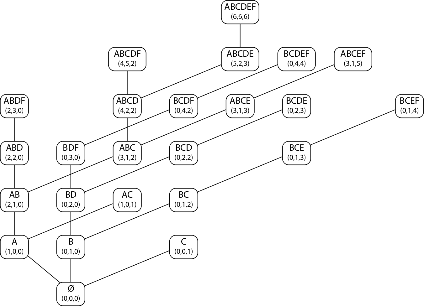
Accessibility also follows from the indexing scheme. For any nonzero vector $v\in\Bbb Z^{k}$, let ${\rm decrement}(v)$ be the vector formed by decreasing the last nonzero coordinate of $v$ by one, and let ${\rm decrement}^{i}(v)$ be the result of iterating the decrement operation $i$ times. Let

and, for any nonempty state $S$ in ${\cal L}_{S}$ let

Figure 6 shows a link from $S$ to ${\rm pred}(S)$ for each state $S$ in the learning space depicted in Figure 5. Then, each iteration of ${\rm decrement}$ causes the image of the vector under the ${\rm up}$ operation either to stay unchanged or to change by the removal of a single item. Since ${\rm pred}(S)$ is defined to be the image after the first iteration that causes a change, it differs from $S$ by the removal of a single item, so the requirement of accessibility is achieved.

Conversely, any learning space satisfying union closure and accessibility can be defined as ${\cal L}_{\Sigma}$ for an appropriate set $\Sigma$ of learning sequences. In a later section we describe how to choose $\Sigma$ to be as small as possible, as the size of $\Sigma$ will be directly related to the efficiency of the algorithms we use to assess learning in ${\cal L}_{\Sigma}$.

As with learning spaces derived from partial orders, we will need to calculate fringes of states. The outer fringe of $S$, the items that may be added to state $S$ to form a new state, is particularly easy to describe: Each state $S\cup\{x\}$ may be formed as the union of the prefixes defining $S$ itself, together with one more prefix $P_{{\rm mex}_{i}(S)}(\sigma_{i})$, so the outer fringe of $S$ is

The inner fringe of $S$, those items in $S$ that may be removed to form another state, is a little more complicated, but still easily expressible using our indexing scheme: it is

The formula ${\rm up}({\rm mex}(S\setminus\{x\}))=S\setminus\{x\}$ is true if and only if $S\setminus\{x\}$ is a state of the learning space, so we may construct the lower fringe by testing whether this formula is true for each member $x$ of $S$.

As with partial orders, we can list all states of a sequence-based learning space by an algorithm based on exploring the tree generated by the predecessor operation we defined earlier; refer back to Figure 6 for a depiction of this tree on an example learning space. Recall that the predecessor of a state is generated by repeatedly reducing the last nonzero coordinate of its ${\rm mex}$ vector until the ${\rm up}$ function maps the reduced vector to a set different from the state itself. In order to reverse this, and find the successors of a state $S$ (that is, the states having $S$ as its predecessor), we need merely perform the following steps:

1. 1.

   Set $p$ to the smallest value of $i$ such that $S$ is the union of prefixes from the first $i$ sequences.

2. 2.

   For each $i\geq p$, such that $\sigma_{i}({\rm mex}_{i}(S))\neq\sigma_{j}({\rm mex}_{j}(S))$ for all $j<i$ (that is, such that the first excluded concept in $\sigma_{i}$ differs from the first excluded concept in all earlier sequences):

   1. (a)

      Let $v$ be formed from ${\rm mex}(S)$ by adding one to its $i$th coordinate.

   2. (b)

      Let $T={\rm up}(v)$ and output $T$.

   3. (c)

      Recursively generate states starting from $T$.

To generate all states in the learning space, we perform a depth first traversal of the states of the space, by applying this procedure recursively starting with the empty set. If $T$ is a successor of $S$, the value of $p$ in the search for the successors of $T$ equals the value of $i$ used when we generated $T$ from its parent $S$; therefore, we may pass these $p$ values through the recursive traversal and avoid calculating them at each step. However, the ${\rm mex}$ values of $S$ and $T$ may differ not just in the $i$th coordinate but also in other coordinates greater than $i$, and must be recalculated. If the learning space is generated by $k$ learning sequences, the time per state is $O(k)$, except for the time to calculate the ${\rm mex}$ value of each new state.

In order to implement our state generation procedure efficiently, we need to be able to calculate the ${\rm mex}$ of each newly generated state. When we defined the ${\rm mex}$ operation we showed that removing an element from a state allows the new ${\rm mex}$ to be calculated easily, but, unfortunately, in the case of the state generation procedure, each new state is generated not by removing an element but by adding one.

To speed up this part of the state generation, we maintain as part of the recursive traversal a collection of long integers, one per learning sequence defining the learning space. In each integer $B_{i}$ we store the number $\sum\{2^{j}\mid\sigma_{j}(i)\in S\}$ representing the set of positions of learning sequence $\sigma_{j}$ that are present in the current state $S$. Each of these integers may be updated in constant time for each step forwards and backwards in the state traversal, and each ${\rm mex}$ calculation may be performed by finding the first zero bit in the binary representation of each integer, which may be performed efficiently using a combination of arithmetic and bitwise boolean operations on the integer. Specifically, the bitwise exclusive or of $B_{i}$ and $B_{i}+1$ is an integer of the form $2^{j}-1$, where $j-1$ is the position of the first zero in $B_{i}$ and should be used as the value of ${\rm mex}_{i}(S)$.

In a programming language without built-in support for integers of arbitrarily large precision, it may be appropriate to replace each value $B_{i}$ in this structure by an array of 32-bit machine integers, each one representing the intersection of $S$ with some 32-member subset of the concepts.

Given the state generation procedure, we can assess the likelihoods of a student knowing each concept using the same Bayesian procedure described for quasi-ordinal spaces.

Specifically, we calculate a likelihood for each state of the space as a product of the prior probability of the state with a set of terms, one term per question asked of the student. As we generate all states, we can calculate each such likelihood as the product of the likelihood of a previously generated state by a single term. The likelihood of a concept is the sum of the likelihoods of the states containing it, and the probability of knowing a concept is this sum normalized by dividing by the sum of likelihoods of all states.

As for the assessment procedure in quasi-ordinal spaces, our state generation procedure operates recursively by adding single concepts to previously generated states. Therefore, if we maintain the sum of likelihoods in each subtree of the recursion, and add each such sums to the total likelihood of the most recently added item, we may compute the sums of likelihoods for all concepts with a single pass over all states of the learning space, in constant additional time per step.

If $\cal F$ is any family of sets, and $P$ is any subset of $\cup\cal F$, we may define the projection

by intersecting each state in ${\cal F}$ with $P$. If $\cal F$ is a learning space, then so is any projection of it. The projection inherits the union closure property of learning spaces from $\cal F$, as $(S_{1}\cap P)\cup(S_{2}\cap P)=(S_{1}\cup S_{2})\cap P$. To prove the accessibility property of learning spaces for a set $S\cap P$, $S\in\cal F$, repeatedly use accessibility in $\cal F$ to remove concepts from $S$ until a concept in $P$ is removed, and let the predecessor of $S\cap P$ be formed by removing the same concept from $S\cap P$.

If $\cal L$ is a quasi-ordinal space, the projection ${\cal L}_{P}$ is also quasi-ordinal order, formed from the restriction of the partial order defining $\cal L$ to the items in $P$. This concept of a learning space derived from a restricted partial order (without the more general notion of projection) is used by ALEKS, as described earlier, to speed up its assessment procedures. Similarly, if $\cal L$ is a learning space derived from a collection of learning sequences, the projection ${\cal L}_{P}$ can be derived from the subsequences formed by listing the items of $P$ in the order they appear in each sequence defining $\cal L$, as shown in Figure 7. Therefore, we may efficiently construct a learning sequence based representation of a projection of a learning space defined by learning sequences. This projected space may not necessarily use the minimum possible number of sequences in its representation, but it uses a number of sequences no more than that of the larger space it was projected from.

The choice of how many concepts to use in modeling knowledge as a learning space is somewhat arbitrary: we may model some areas of knowledge coarsely, as a relatively small set of concepts, and others more finely using many concepts. We do not expect our assessment of the likelihood that a student knows a given concept to vary significantly based on the choice of how coarsely the space is modeled. Therefore, though there is little mathematical justification for this simplification, we may greatly speed up our knowledge assessment routines by projecting to a space consisting only of the relevant concepts for the assessment: those we wish to assess, and those for which we have answers.

To be specific, suppose that $Q$ is a set of concepts on which we have tested a student’s knowledge, in a learning space $\cal L$, and $x$ is a concept for which we wish to infer a likelihood of the student’s knowledge. Rather than applying the state-generation based assessment algorithm to the whole learning space $\cal L$, we may apply it to the projected space ${\cal L}_{Q\cup\{x\}}$.

Mathematically, in order to get assessment results in the projection equal to the results in the original space $\cal L$, we would need to use a prior probability in each projected state $S$ equal to the sum of the prior probabilities of the states in $\cal L$ that project to $S$. For instance, if we are using the uninformative prior for $\cal L$, in which we assume that each state is equally likely to occur, then in the projection we should use a prior in which the probability for each state $S$ is proportional to the number of states in $\cal L$ that project to $S$. However, even for the uninformative prior, this problem of quickly calculating numbers of states seems quite difficult. Instead, we propose performing the evaluation in the projected space ${\cal L}_{Q\cup\{x\}}$ as if it were the whole space. The results of the likelihood calculation in this projection may differ from those of the calculation in the whole space $\cal L$, but there seems little reason in principal to view one of the results as more reliable than the other, and if $Q$ is small then the projected assessment may be much more efficient than the assessment in the original space. If $Q$ is so small that ${\cal L}_{Q}$ does not provide adequate coverage of the learning space, however, the assessment may be less informative than that in $\cal L$; for instance, concepts occurring in very few states of the learning space would have very low likelihood when assessed in $\cal L$ with $Q=\emptyset$ but $50\%$ likelihood when assessed in ${\cal L}_{\{x\}}$. This problem of a too-small sample losing information about the number of states containing concept $x$ may be ameliorated by adding a small random sample $R$ of the learning space concepts to $Q$; that is, if we perform the assessment in ${\cal L}_{Q\cup R\cup\{x\}}$ in place of ${\cal L}_{Q\cup\{x\}}$, we can gain an accurate estimate of the number of states containing $x$ even when $Q$ is empty or near-empty.

One unfortunate feature of computing assessments in ${\cal L}_{Q\cup\{x\}}$ rather than $\cal L$ is that it requires a separate run of the state generation procedure for each separate concept $x$, while the assessment procedure in ${\cal L}$ involves only a single run of the state generation procedure. It seems likely that, if we wish to compute likelihoods for all concepts in the knowledge space, a faster procedure would be to partition the concepts into small collections $C_{i}$, and to use the state generation based assessment procedure on ${\cal L}_{Q\cup C_{i}}$ to compute likelihoods for each concept in $C_{i}$. If $C_{i}$ is chosen to be too small, this would involve many runs of the procedure, while if $C_{i}$ is chosen to be too large, then the procedure will list too many states, so there is likely some optimal intermediate value (perhaps depending on the size of $Q$) to use for the size of the collections $C_{i}$ in order to make this projection based assessment procedure run at optimal speed. The tradeoffs of runtime versus collection size would need to be found by experimental analysis beyond the scope of this chapter. However, if the collections $C_{i}$ are chosen randomly rather than as distance based clusters, they would also perform the same function as the set $R$ above of making the states of the projected space more representative of the numbers of states in the original space. Thus, it may be desirable for the accuracy of the assessment to chose $C_{i}$ larger than an analysis based only on algorithmic efficiency would suggest.

We are hopeful that the speedup provided by this projection based assessment method, relative to the more naive state generation based assessment used by the current version of ALEKS, would allow student assessment to proceed in a single pass involving all concepts in the learning space, rather than the multipass clustering based approach used in the current version of ALEKS. In outline, the procedure would proceed as follows:

1. 1.

   Initialize $Q$ to $\emptyset$.

2. 2.

   Repeat:

   1. (a)

      Partition the concepts of the learning space randomly into collections $C_{i}$.

   2. (b)

      For each $C_{i}$, generate the states of ${\cal L}_{Q\cup C_{i}}$ and apply the assessment algorithm to compute likelihoods for each concept in $C_{i}$.

   3. (c)

      If all concepts have likelihoods bounded away from $50\%$, terminate the assessment procedure.

   4. (d)

      Choose a concept $x$ with likelihood as close as possible to $50\%$, assess the student’s knowledge of $x$, and add $x$ to $Q$.

As discussed above, the choice of how large to make the collections $C_{i}$ is left undetermined by this algorithm, and involves a tradeoff between algorithmic efficiency and assessment accuracy.

We considered also an alternative assessment procedure to the one described in the previous section, in which we maintain sets of concepts $K$ and $U$ which we believe the student to know or not know respectively, and restrict the state space search used in the assessment algorithm to only those states consistent with $K$ and $U$. That is, rather than totalling likelihoods for all states in ${\cal L}$, we only total those likelihoods in the states of ${\cal L}$ that project to $K$ in ${\cal L}_{K\cup U}$; all other states are assumed to have a priori probability zero of being the actual state of knowledge of the student. As $K$ and $U$ grow through the course of the assessment, this could lead to a significant reduction in the number of states that need to be listed. However, some form of sampling and assessment based on the projection of $\cal L$ onto the sample would still be needed in order to achieve adequate performance in the earlier stages of the algorithm when $K$ and $U$ are small. One possible structure for such an algorithm is shown below.

1. 1.

   Initialize $K$ and $U$ to empty.

2. 2.

   Repeat:

   1. (a)

      Choose a sample $S$ of the concepts in $\cup{\cal L}\setminus(K\cup U)$.

   2. (b)

      Repeat:

      1. i.

         Use the likelihood calculation algorithm on ${\cal L}_{S\cup K\cup U}$, restricted to only those states that project to $K$ in ${\cal L}_{K\cup U}$, to compute likelihoods for $S$.

      2. ii.

         If no concept in $S$ has likelihood near $50\%$, terminate the inner loop.

      3. iii.

         Choose a concept with likelihood as close to $50\%$ as possible and test the student’s knowledge of that concept.

   3. (c)

      Add the concepts of $S$ with likelihoods significantly larger than $50\%$ to $K$, and add the concepts of $S$ with likelihoods significantly smaller than $50\%$ to $U$.

   4. (d)

      If all concepts of ${\cal L}$ are in $K$ or $U$, terminate the algorithm.

This algorithm appears to improve on the previous section’s algorithm by requiring only a single pass through the states of a projected learning space per question asked of the student. However we see several significant potential problems with this approach that stopped us from investigating it in greater detail. First, the assignment of states to $K$ and $U$ is made with certainty, making a Bayesian interpretation of this algorithm problematic. Second, while it is possible to generate the states consistent with $K$ and $U$ in relatively small time per state, we have not been able to find an algorithm for this task that is as efficient as the one for listing all states in a learning space. And third and most troubling, if the algorithm ever reaches a situation where the projection ${\cal L}_{K\cup U}$ does not contain $K$ as a state, the algorithm will fail by dividing by zero in the calculation of the concept likelihoods, so it is not robust against inaccuracies in the learning space model or the assessment algorithm.

Nevertheless if we wish to implement such an algorithm we must find the set of states in $\cal L$ project to $K$ in ${\cal L}_{S\cup K\cup U}$, in order to perform the likelihood calculations of the algorithm. We may impose a tree structure on this set of states by choosing a learning sequence $\sigma$ of $\cal L$ that contains as a prefix the union of the states that project to $K$, and defining the parent of any state $S$ to be the state formed by adding to $S$ the first missing concept in $\sigma$. A reverse search algorithm that reverses this parent relation and traverses this tree can list all states that project to $K$, in a small number of steps per listed state, but we have not found a way to make this algorithm as efficient as the one we gave earlier for listing all states in a learning space. We omit the details.

We have provided above a method based on projection that does not involve the distance-based clustering currently used in ALEKS. However, it may still be of interest to define a distance function on the concepts of the learning space. For instance, as we have discussed above, clustering based on distance may be useful for the partition into collections $C_{i}$ in our projection based assessment algorithm. In addition, the distance from some previously assessed state may be an important ingredient in the prior probability distribution on learning space states used by the knowledge assessment algorithm.

The learning sequences we use to define our learning spaces provide a natural family of distances: if we interpret each concept’s position in each sequence as a coordinate, all such positions form a vector corresponding to the concept in $\Bbb Z^{k}$, and we may use any $L_{p}$ metric on this collection of vectors. We did not investigate more carefully the choice of metric to determine the value of $p$ that would work best for knowledge assessment applications.

A chain in a partial order is a set of items that are all comparable to each other; any chain can be ordered into a sequence $x_{0},x_{1},\ldots$ such that $x_{i}<x_{j}$ if and only if $i<j$. A chain cover is a set of chains that together include all items in the order. Similarly, an antichain in a partial order is a set of items no two of which are comparable to each other, so that the partial order places no restrictions on their ordering. The width of a partial order is the maximum cardinality of any of its antichains. It is well known (Dilworth’s Theorem) that, for any partial order, the width is also equal to the minimum number of chains in a chain cover.

For instance, the partial order depicted on the left of Figure 1 can be covered by two chains, $\{A,C,E,G\}$ and $\{B,D,F,H\}$. It also has many antichains of two concepts, for instance $\{A,B\}$. Therefore, its width is exactly two. There cannot be any antichain of three or more concepts, nor is there a single chain that covers all its concepts.

An optimal chain decomposition of a given partial order may be found by a technique based on bipartite graph matching (Figure 8). The far left of the figure shows the same partial order as the one in Figure 1, and the center left shows a bipartite graph derived from this order. In the bipartite graph, we have two vertices for each item in the partial order, one on the left and one on the right. We draw an edge from the vertex labeled $x$ on the left to the vertex labeled $y$ on the right whenever $x<y$. In general this graph may be disconnected, and have vertices incident to no edges; these complications cause no difficulty for our algorithms. A matching in a graph is a set of edges, at most one edge incident on any vertex, and a maximum matching is a matching maximizing the total number of edges in the set. A maximum matching of the graph in the figure is shown in center right. From any matching in this graph, we may derive a chain cover, by including in the same chain any two items in the partial order that form the two endpoints of a matched edge; such a cover, for the matching in the figure, is shown on the far right. In a partial order with $n$ items, matchings with $k$ matched edges correspond to chain covers with $n-k$ chains, so the minimum chain cover can be found from the maximum matching.

Hopcroft and Karp (1973) showed how to find a maximum matching in a bipartite graph with $n$ vertices and $m$ edges in time $O(mn^{1/2})$; for partial orders with $n$ items this translates to an $O(n^{5/2})$ time bound for finding an optimal chain decomposition and therefore finding the width. A maximum antichain may also be found in the same amount of time; we omit the details as they are not necessary for our learning space application.

Recall that a chain is a totally ordered collection of objects in a partial order. Therefore, a chain of states of a learning space consists of a nested family of sets. We show here, for $\cal C$ any chain of states in learning space $\cal L$, how to find a learning sequence $\sigma$ in $\cal L$ such that each state of $\cal C$ is a prefix of $\sigma$. We may assume without loss of generality that $C$ contains $\emptyset$ and $\cup\cal L$.

To find $\sigma$, sort the sets in $\cal C$ by size:

We will build up $\sigma$ in stages; after the $i$th stage, we will have chosen values for $\sigma_{0},\sigma_{1},\ldots\sigma_{|S_{i}|-1}$ such that all sets $S_{j}$, $j\leq i$, are prefixes of the chosen sequence of values and such that all prefixes of the sequence are states in $\cal L$. Initially, the empty sequence satisfies this requirement for $i=0$.

In stage $i$, we will have already generated a sequence for the elements of $S_{i-1}$. By the accessibility property of learning spaces, we can also generate a sequence $\tau_{0},\tau_{1},\ldots\tau_{|S_{i}|-1}$ of the elements of $S_{i}$, such that each prefix of this sequence is a state in $\cal L$. We then form our new longer sequence of $\sigma_{j}$ values by concatenating the subsequence of the $\tau_{j}$’s not already chosen as $\sigma_{j}$’s onto the end of the previously chosen $\sigma_{i}$’s. This concatenation preserves the property that the sets $S_{j}$, $j<i$, are all prefixes of the new sequence, and now $S_{i}$ itself is the prefix consisting of the whole concatenation. In addition, each prefix of the new sequence is the union of a prefix of the old sequence of $\sigma_{j}$’s and of a prefix of the sequence of $\tau_{j}$’s, and therefore by the union closure property of learning spaces is a state of $\cal L$.

Once we have completed the final stage of this process, for $S_{k}=\cup\cal L$, the ordering on $\sigma$ provides the desired learning sequence. We refer to the existence of this learning sequence $\sigma$ as the chain property of learning spaces.

In general, the algorithm described here involves a number of predecessor calculations equal to the sum of the cardinalities of the sets in the chain. For learning spaces derived from partial orders on $n$ concepts, described by Hasse diagrams with $m$ edges, a faster algorithm is possible, based on a standard method for performing topological ordering via depth first search: we sort the elements in descending order by the size of the smallest chain set they belong to, and perform a depth first traversal of the Hasse diagram, initiating the traversal at the elements in the sorted order. The desired learning sequence is the reverse of a postorder numbering for this traversal. Thus, after ordering the elements by the smallest containing chain sets, the remaining algorithm takes time $O(m+n)$.

The base of a union-closed family of sets is a minimal subfamily such that any member of the family can be reconstructed as a union of members of the subfamily. For antimatroids (union-closed accessible families) there is a particularly easy construction of a base.

Define a predecessor of set $S$ in antimatroid $\cal A$ to be any set $T=S\setminus\{x\}$ that also belongs to $\cal A$. If $S$ has zero predecessors, and $\cal A$ is accessible, then $S$ must be empty and can be reconstructed as an empty union of sets no matter what base is chosen. And, if $S$ has two or more predecessors, each of which can be reconstructed as a union of sets in the base, then $S$ itself can be reconstructed as the union of any two of its predecessors. Thus in either of these two cases $S$ cannot belong to a base. However, if $S$ has only a single predecessor $T$, then any proper subset of $S$ is also a subset of $T$: by the chain property, there must be a learning sequence containing the proper subset and $S$ itself as prefixes, and the predecessor of $S$ on that sequence must be $T$. Therefore, in this case, any union of subsets of $S$ forms a subset of $T$ and cannot equal $S$, so $S$ must belong to every base. From these considerations we see that any antimatroid $\cal A$ has a unique base ${\cal B}({\cal A})$ consisting of the sets that have a single predecessor. We view ${\cal B}({\cal A})$ as forming a partial order by set inclusion: if $S$ and $T$ are both sets in the base, then $S<T$ in the partial order if and only if $S\subset T$.

In a learning space $\cal L$ derived from a partial order, the base sets have the form $S_{x}=\{y\mid y<x\}\cup\{x\}$. For, the only predecessor of $S_{x}$ is $S_{x}\setminus\{x\}$, but any set not of this form is either empty or has two or more independent maximal elements, each of which can be removed to form a predecessor. Also, $S_{x}\subset S_{y}$ if and only if $x<y$. Thus the base sets correspond one-for-one with the concepts of $\cal L$ and the partial order on ${\cal B}({\cal L})$ is isomorphic to the partial order on concepts. However, for learning spaces not derived from partial orders, ${\cal B}({\cal L})$ may contain many more sets than there are concepts in the learning space. Figure 9 depicts the partial order formed by the base of the learning space depicted in Figure 5; this base has seven sets although it describes a learning space on only six concepts.

It will also be of interest to find the base of a learning space ${\cal L}_{\Sigma}$ defined from a set $\Sigma$ of learning sequences. For learning spaces of this type, the only states that could be in a base are the prefixes of $\Sigma$: any state that is not a prefix can be formed as a union of smaller sets, and therefore cannot be in the base. If state $S$ is a prefix of one of our defining sequences $\sigma_{i}$, with $x$ as the latest concept in that prefix, then $S$ is a base if and only if the position of $x$ in each other $\sigma_{j}$ is either the same as its position in $\sigma_{i}$ or later than the minimum excluded element of $S$ in $\sigma_{j}$. For, if this is so, no other symbol can be removed from $S$ leaving a valid state, while if it is not true then there exists a symbol $y$ such that ${\rm mex}(S\setminus\{y\})$ is not dominated by ${\rm mex}(S\setminus\{x\})$, and the $y$ for which ${\rm mex}(S\setminus\{y\})$ is maximal among other such vectors may be removed to form another valid state. Thus, we may test whether $S$ is a base state, once its ${\rm mex}$ has been calculated, in time proportional to the number of defining sequences. We may find the base by listing the prefixes of each defining sequence, in order from longer prefixes to smaller ones so that we may more efficiently update the ${\rm mex}$ values, and applying this test to each prefix. In a space with $n$ concepts, defined by $k$ sequences, this base generation algorithm takes time $O(nk^{2})$ and generates at most $kn$ base sets.

If $\Sigma$ is a collection of learning sequences for a learning space $\cal L$, then ${\cal L}_{\Sigma}\subset{\cal L}$. When does the learning space ${\cal L}_{\Sigma}$ derived from $\Sigma$ equal ${\cal L}$?

If every base set for $\cal L$ is a prefix of $\Sigma$, then all states in $\cal L$ can be formed as unions of those base members, and ${\cal L}_{\Sigma}={\cal L}$. Conversely, if some set $B\in{\cal B}({\cal L})$ is not a prefix of $\Sigma$, then $B$ can not be reconstructed as a union of any other sets in $\cal L$, let alone of the prefixes of $\Sigma$, and ${\cal L}_{\Sigma}\neq{\cal L}$.

The prefixes of a single learning sequence form a chain in the set inclusion ordering, and the base elements within that family form a chain in ${\cal B}({\cal L})$. Conversely, if we have any chain in ${\cal B}({\cal L})$, we may use the chain property to form from it a learning sequence containing as prefixes all chain members. Thus, a set $\Sigma$ of learning sequences determines the learning space ${\cal L}_{\Sigma}={\cal L}$ if and only the base prefixes for each chain form a chain cover of ${\cal B}({\cal L})$. The minimum number of learning sequences needed to determine the learning space is the minimum number of chains in a chain cover of ${\cal B}({\cal L})$, that is, its width.

We are now ready to describe an algorithm that, given a learning space $\cal L$, calculates its convex dimension and finds a minimum family $\Sigma$ of learning sequences such that ${\cal L}_{\Sigma}=\cal L$. The algorithm simply performs the following steps:

1. 1.

   Find the base ${\cal B}({\cal L})$.

2. 2.

   Use bipartite matching to find a minimum chain cover of ${\cal B}({\cal L})$.

3. 3.

   Use the chain property to extend each chain in the cover to a learning sequence for $\cal L$.

4. 4.

   Let $\Sigma$ be the set of learning sequences so constructed. The convex dimension is the number of learning sequences in $\Sigma$.

If only the convex dimension and not the learning sequences themselves is desired, step 3 can be omitted. Assuming a suitably algorithmic implementation of the underlying learning space $\cal L$, all of these steps may be performed in time polynomial in $|{\cal B}|$ and in the number of concepts in $\cal L$, both of which we expect to be far smaller than the total number of states in $\cal L$.

For learning spaces derived from partial orders on $n$ concepts, described by Hasse diagrams with $m$ edges, the first step is trivial, and the second step takes time $O(n^{5/2})$. There $k\leq n$ chains in the cover, and any single chain may be extended to a learning sequence in time $O(m)$. Thus, the third step can be implemented in time $O(mk)$, and the overall algorithm takes time $O(n^{5/2}+mk)$. indexworst case time complexity

Once a minimum family $\Sigma$ of learning sequences for $\cal L$ has been generated, we may redefine $\cal L$ as ${\cal L}_{\Sigma}$, and use our computational representation based on learning sequences for any future calculations in $\cal L$.

State $S$ may be removed from learning space $\cal L$ if, and only if, it satisfies all of the following requirements:

1. 1.

   $S$ is in the base of $\cal L$.

2. 2.

   $S\neq\cup\cal L$.

3. 3.

   No set $S\cup\{x\}$, $x\notin S$, is in the base of $\cal L$.

If $S$ were not in the base, it could be formed as the union of other sets in $\cal L$, and removing it would violate union closure. Similarly, if some set $S\cup\{x\}$ were in the base, removing $S$ would violate accessibility for that set. On the other hand, if the requirements above are all satisfied, then the space formed by removing $S$ from $\cal L$ satisfies union closure and accessibility, and therefore forms a valid learning space. The base of this new space consists of the remaining base members of $\cal L$, together with certain sets of the form $S\cup\{x\}$, from which we may use our concise representation algorithm to construct a representation of ${\cal L}\setminus\{S\}$ in terms of a small number of learning sequences. All removable sets may be found efficiently, for spaces constructed from learning sequences, by listing all base sets and testing the above conditions.

The generation of sets that may be added to a learning space $\cal L$ to form an augmented learning space is somewhat more problematic, as it cannot be done efficiently by generating and modifying the base of $\cal L$. If $S$ is any state of $\cal L$, the sets $S\cup\{x\}$ that can be added to $\cal L$ are exactly those for which $x$ belongs to the intersection of the outer fringes of states of the form $S\cup\{y\}$. For, such an $x$ cannot belong to a state $S\cup\{x\}$ already, as the outer fringe of that state would not contain $x$; adding $S\cup\{x\}$ as a state preserves accessibility through $S$; and membership in the intersection ensures the union closure property of the augmented space. On the other hand, if $x$ does not belong to the outer fringe of some $S\cup\{y\}$, then $S\cup\{x\}$ cannot be added to $\cal L$, as the resulting space would not contain the union of $S\cup\{x\}$ and $S\cup\{y\}$.

Thus, to generate all sets that may be added to $\cal L$, we need merely list all states of $\cal L$, list for each state $S$ the states $S\cup\{y\}$ by computing the outer fringe of $S$, and intersect the outer fringes of the states $S\cup\{y\}$. Each such set is listed only once by this procedure, as the set $S$ for which it is listed must be unique or it would already belong to $\cal L$ by union closure. If we add a set $S\cup\{x\}$ as a new state to a learning space $\cal L$, the base of the new learning space consists of the newly added set, together with all base members of $\cal L$ that are not of the form $S\cup\{x,y\}$.

We discussed briefly earlier the possibility of forming reduced state spaces by inverting projections: if we believe that a student knows the concepts in a set $K$, and that the student doesn’t know the concepts in a set $U$, what structure can we see in the subset of learning space states ${\cal L}(K,U)$ consistent with those beliefs? The states in ${\cal L}(K,U)$ are exactly those that project to $K$ in ${\cal L}_{K\cup U}$. Therefore, we can view ${\cal L}(K,U)$ as a fiber of the projection, the inverse image of $K$. What combinatorial properties does such a fiber have?

We observe that, more generally, if $\cal F$ is any family of sets, and ${\cal F}(K,U)$ denotes the subfamily of sets in $\cal F$ that are supersets of $K$ and disjoint from $U$, then closure under unions or intersections of $\cal F$ leads to the same property of ${\cal F}(K,U)$. For, taking the union or intersection of two sets in ${\cal F}(K,U)$ cannot form a set that is not a superset of $K$ or not disjoint from $U$. Similarly, if $\cal F$ is well-graded, then ${\cal F}(K,U)$ inherits the same property. Learning spaces derived from partial orders can be characterized as well-graded set families that are closed under unions and intersections, so if $\cal L$ is a learning space formed in this way, so is ${\cal L}(K,U)$.

For general learning spaces, however, a fiber need not itself form a learning space. For instance, for the learning space $\cal L$ of Figure 4, the projection ${\cal L}_{\{B\}}$ has two states, $\emptyset$ and $\{B\}$, but the inverse image ${\cal L}({B},\emptyset)$ of $\{B\}$ is the family of three states $\{\{A,B\},\{A,B,C\},\{B,C\}\}$, which does not form a learning space as it fails the accessibility property. However, the fiber of a learning space projection is well-graded and closed under unions, and therefore forms a closed medium (Falmagne and Ovchinnikov, 2002).

If $\cal L$ is a learning space, we define an upper subfamily ${\cal L}^{+}$ of $\cal L$ to be a subset of the states of $L$, such that if $S\subset T$ are two states of $\cal L$ with $S\in{\cal L}^{+}$ then $T\in{\cal L}^{+}$.

Figure 10 shows a well-graded union-closed set family $\cal F$ that cannot be an upper subfamily ${\cal L}^{+}$ of a learning space ${\cal L}$. For $\cal L$ would have to contain a singleton as one of its states; by symmetry we can assume without loss of generality that this singleton is $\{a\}$. Then $\cal L$ would contain $\{a\}\cup\{d,e\}=\{a,d,e\}$. But $\{a,d,e\}$ is not in $\cal F$ while its subset $\{d,e\}$ is. Therefore, the family of fibers of projections of learning spaces is a proper subclass of the family of closed media.

This result gives us hope that there exists a simple combinatorial description of the set families that form upper subfamilies of learning spaces. However, finding the smallest learning space for which $\cal F$ is an upper subfamily is considerably more difficult.

If ${\cal L}_{1}$ and ${\cal L}_{2}$ are two learning spaces on the same set of concepts, we may define a join operation combining the two into a single larger learning space:

This operation is commutative, associative, and idempotent (that is, ${\cal L}\sqcup{\cal L}={\cal L}$ for any learning space $\cal L$); therefore it forms a semilattice though not, in general, a medium.

The problem of computing the convex dimension of a learning space ${\cal L}$, and of representing ${\cal L}$ via a minimum number of learning sequences, can be viewed in this way as expressing $\cal L$ as the join of a small number of simpler learning spaces: if we define a totally ordered learning space to be a learning space formed from a single learning sequence, then ${\cal L}$ has convex dimension at most $K$, and can be represented via $K$ learning sequences, if and only if it is the join of at most $K$ totally ordered learning spaces. The totally ordered learning spaces form the smallest subclass of learning spaces such that all learning spaces can be represented as joins of learning spaces in the subclass, for a learning space is irreducible for the join operation if and only if it is totally ordered.

The algorithmic success of our learning sequence representation motivates us to seek more powerful forms of decompositions of learning spaces as joins of broader classes of learning spaces. For, if $\cal L$ can be represented as a join of a small number of learning spaces ${\cal L}_{i}$, each of which in turn has an efficient algorithmic representation, then it seems likely that we may also perform various algorithms efficiently for $\cal L$ itself, with an efficiency depending in part on the number $K$ of learning spaces used to represent $\cal L$. For instance, with such a representation, a base for $\cal L$ may be found as a subfamily of the union of bases of ${\cal L}_{i}$. But to use representions based on joins of special classes of learning spaces, we need to be able to find such representations efficiently. We have already shown that, if $\cal F$ is the family of totally ordered learning spaces, then a representation of any learning space as the join of a minimum number of members of $\cal F$ can be found efficiently. For which other families $\cal F$ is such efficient decomposition possible?

The same proof shows that the problem remains hard when $K$ is fixed to any constant greater than two. A similar reduction (omitting the concepts $\ell_{e}$) shows that it is NP-complete to represent a learning space as a join of three or more hierarchies, where a hierarchy is defined as a quasi-ordinal learning space for an order the Hasse diagram of which has at most one outgoing edge per concept. A hierarchy can be characterized as a learning space each two base sets of which are either disjoint or nested, so one can test whether a learning space $\cal L$ is a join of two hierarchies by forming a graph in which we connect two base sets of $\cal L$ by an edge whenever they do not satisfy this condition and testing whether this graph is bipartite; we omit the details. We have not yet determined whether it is possible to test efficiently whether a given learning space is the join of two quasi-ordinal spaces.

We have described learning spaces (or antimatroids) here as union-closed accessible families of sets, and they are also commonly formalized as prefix-closed formal languages satisfying a certain exchange axiom (Korte et al., 1991). Media theory (Falmagne and Ovchinnikov, 2002; Eppstein et al., 2007) leads to alternative formalizations involving geometric graphs and finite automata, and previous work on drawing antimatroids (Eppstein, 2006) leads to a characterization in terms of arrangements of translated orthants. But it turns out that antimatroids also have a fairly natural algebraic characterization. That is, we view antimatroids in terms of the algebraic properties of their union operation rather than as systems of explicit sets and elements. Perhaps this is not surprising, as the first work on antimatroids (Dilworth, 1940) characterized them algebraically in terms of lattices, but we use semilattices instead.

The model for this is an algebraic description of semilattices and quasi-ordinal spaces (equivalently, finite distributive lattices or finite lattices of sets). A monoid consists of an associative binary operation (such as multiplication or string concatenation or function composition) on a set of objects, together with an identity object for the operation (such as, respectively, 1 or the empty string or the identity function); here we write the monoid operation as multiplication. A semilattice is a monoid that is commutative ($xy=yx$ for all $x,y$) and idempotent ($x^{2}=x$ for all $x$). The divisibility relation on a semilattice ($x|y$ if, for some $z$, $xz=y$) forms a partial order, and the semilattice operation can be interpreted as a join or least upper bound operation for that partial order. By analogy with ring theory we can define an irreducible object in a semilattice to be an $x$ such that if $x=yz$ then $x=y$ or $x=z$, and we can define a prime object in a semilattice to be an $x$ such that if $x|yz$ then $x|y$ or $x|z$. Lattices are normally defined in terms of two compatible semilattices, one for joins and one for meets, but as we see below the concepts of irreducibility and primality allow us to define finite lattices of sets in terms of the join operation only.

Antimatroids lie between semilattices and quasi-ordinal spaces in generality, so it seems natural to axiomatize them similarly. However, it doesn’t appear to work to use primes and irreducibles as with lattices: that axiomatization corresponds set elements with the minimum lattice object containing that element, but in antimatroids there may be no unique minimum object. Instead it works better to turn things upside down, and correspond elements with the maximum object not containing the element.

By analogy, in any semilattice, we define $s$ to be singular iff it has a single successor $t$, such that $s|t$ and, for any $x$, if $s|x$ then $s=x$ or $t|x$. We identify any object $x$ in the semilattice with the set $N(x)$ of singular objects that $x$ does not divide.

References

- Avis and Fukuda (1996) D. Avis and K. Fukuda. Reverse search for enumeration. Discrete Applied Mathematics, 65:21–46, 1996.
- Birkhoff (1937) G. Birkhoff. Rings of sets. Duke Mathematical Journal, 3:443–454, 1937.
- Boyd and Faigle (1990) E.A. Boyd and U. Faigle. An algorithmic characterization of antimatroids. Discrete Applied Mathematics, 28:197–205, 1990.
- Dilworth (1940) R.P. Dilworth. Lattices with unique irreducible decompositions. Annals of Mathematics, 41:771–777, 1940.
- Doble et al. (2001) C.W. Doble, J.-P. Doignon, J.-Cl. Falmagne, and P.C. Fishburn. Almost connected orders. Order, 18(4):295–311, 2001.
- Doignon and Falmagne (1999) J.-P. Doignon and J.-Cl. Falmagne. Knowledge Spaces. Springer-Verlag, Berlin, Heidelberg, and New York, 1999.
- Dowling (1993) C.E. Dowling. Applying the basis of a knowledge space for controlling the questioning of an expert. Journal of Mathematical Psychology, 37:21–48, 1993.
- Eppstein (2005a) D. Eppstein. Algorithms for drawing media. In Graph Drawing: 12th International Symposium, GD 2004, New York, NY, USA, September 29–October 2, 2004, volume 3383 of Lecture Notes in Computer Science, pages 173–183, Berlin, Heidelberg, and New York, 2005a. Springer-Verlag.
- Eppstein (2005b) D. Eppstein. The lattice dimension of a graph. European Journal of Combinatorics, 26(6):585–592, 2005b.
- Eppstein (2006) D. Eppstein. Upright-quad drawing of -planar learning spaces. In Graph Drawing: 14th International Symposium, GD 2006, Karlsruhe, Germany, September 18–20, 2006, Lecture Notes in Computer Science, Berlin, Heidelberg, and New York, 2006. Springer-Verlag.
- Eppstein et al. (2007) D. Eppstein, J.-Cl. Falmagne, and Ovchinnikov S. Media Theory. Springer-Verlag, Berlin, Heidelberg, and New York, 2007.
- Falmagne and Doignon (1988) J.-Cl. Falmagne and J-P. Doignon. A class of stochastic procedures for the assessment of knowledge. British Journal of Mathematical and Statistical Psychology, 41:1–23, 1988.
- Falmagne and Ovchinnikov (2002) J.-Cl. Falmagne and S. Ovchinnikov. Media theory. Discrete Applied Mathematics, 121:83–101, 2002.
- Falmagne et al. (1990) J.-Cl. Falmagne, M. Koppen, M. Villano, J.-P. Doignon, and L.. Johanessen. Introduction to knowledge spaces: how to build, test and search them. Psychological Review, 97:204–224, 1990.
- Fredman and Khachiyan (1996) Michael L. Fredman and Leonid Khachiyan. On the complexity of dualization of monotone disjunctive normal forms. Journal of Algorithms, 21(3):618–628, 1996.
- Hopcroft and Karp (1973) J.E. Hopcroft and R.M. Karp. An algorithm for maximum matchings in bipartite graphs. SIAM J. on Computing, 2(4):225–231, 1973.
- Jerrum et al. (2001) M. Jerrum, A. Sinclair, and E. Vigoda. A polynomial-time approximation algorithm for the permanent of a matrix with non-negative entries. In Proc. 33rd ACM Symp. on Theory of Computing, pages 712–271, 2001.
- Kempner and Levit (2003) Y. Kempner and V.E. Levit. Correspondence between two antimatroid algorithmic characterizations. Electronic preprint math.CO/0307013, arXiv.org, 2003.
- Korte et al. (1991) B. Korte, L. Lovász, and R. Schrader. Greedoids. Number 4 in Algorithms and Combinatorics. Springer-Verlag, 1991.
- Thiéry (2001) N. Thiéry. Dynamically Adapting Knowledge Spaces. PhD thesis, Univ. of California, Irvine, School of Social Sciences, 2001.
- Yannakakis (1982) M. Yannakakis. The complexity of the partial order dimension problem. SIAM J. Alg. Disc. Meth., 3(3):351–358, September 1982.