The KP hierarchy, branched covers, and triangulationsThanks:  ^∗Department of Combinatorics and Optimization, University of Waterloo, Waterloo, Ontario, Canada.;
  ipgoulden@uwaterloo.caThanks:  ^†Department of Combinatorics and Optimization, University of Waterloo, Waterloo, Ontario, Canada.;
  dmjackso@math.uwaterloo.ca

The KP (Kadomtsev-Petriashvili) hierarchy is a completely integrable system of quadratic, partial differential equations for an unknown function $F$, that generalizes the KdV hierarchy. Over the last two decades, there has been strong interest in the relationship between integrable systems and moduli spaces of curves. This began with Witten’s Conjecture [W] for the KdV equations, proved by Kontsevich [Ko] (and more recently by a number of others, including [KL]). Pandharipande [P] conjectured that solutions to the Toda equations arose in a related context, which was proved by Okounkov [Ok], who also proved the more general result that a generating series for what he called double Hurwitz numbers satisfies the KP-hierarchy. Kazarian and Lando [KL], in their recent proof of Witten’s conjecture, showed that it is implied by Okounkov’s result for double Hurwitz numbers. More recently, Kazarian [Ka] has given a number of interesting results about the structure of solutions to the KP hierarchy.

To fix ideas, the first few of the countable equations in the KP hierarchy are

where

We have found [MJD] to be an accessible source for the KP hierarchy, and note that the variables $p_{i}$ that we use in this paper are related to the variables used in [MJD] by $p_{i}=i\,x_{i}$, $i\geq 1$. Thus the partial derivatives in our equations (with respect the $p_{i}$’s) are scaled differently from those in [MJD] (which are with respect to the $x_{i}$’s).

There is a powerful characterization of the solutions to the KP hierarchy that is particularly convenient from an algebraic combinatorics or geometric point of view. This is well-known in the integrable systems literature (see, e.g., Ch. 10 of [MJD]), and concerns linear combinations of Schur symmetric functions (here the variables $p_{1},p_{2},\ldots$ are the power sum symmetric functions). The characterization states that the coefficients in the linear combination of Schur functions satisfy the Plücker relations from geometry. In the remainder of Section 1 (Sections 1.2 – 1.4), we give the background required to state this characterization precisely (Theorem 1.3).

In Section 2, we apply the Schur function characterization to give an explicit solution to the KP hierarchy (as Theorem 2.3) in terms of products of a countable set of variables indexed by the integers, recording content. Content is a combinatorial parameter for partitions that often appears in expressions for symmetric functions (which are themselves naturally indexed by partitions). We establish this result as an immediate corollary of Theorem 2.2, in which we give a content product solution to the Plücker relations. The content product solution to the KP hierarchy has previously been given by Orlov and Shcherbin [OS], using different methods. In Section 3 we turn to algebraic combinatorics. We consider a general set of transitive ordered factorizations in the symmetric group, and prove that a particular generating function for the numbers of such factorizations satisfies the KP hierarchy. This is our main result, given as Theorem 3.1. In Section 4, we consider the geometrical interpretation of transitive ordered factorizations, in terms of branched covers. Thus in Section 4.2, as a corollary of our main result, we obtain Okounkov’s [Ok] result, that the generating series for double Hurwitz numbers satisfies the KP hierarchy (Theorem 4.1). In Section 4.3 we consider a new class of geometric numbers, called $m$-hypermap numbers, and prove that the generating series for these satisfies the KP hierarchy (Theorem 4.2). In Section 4.4, we prove that the $m$-hypermap numbers are polynomials in $m$, with the double Hurwitz numbers as the leading coefficient (Theorem 4.3), and speculate that the rich geometry for the latter might extend to the former. Then in Section 5, we specialize further to establish that generating series for the numbers of rooted hypermaps (Theorem 5.1) and rooted maps in an orientable surface (Theorem 5.2) are solutions to the KP hierarchy. In Section 5.3, we conclude by using one of the KP equations to give a new and remarkably simple recurrence for triangulations in an orientable surface of specified genus, with a given number of faces (Theorem 5.4).

If ${\lambda}_{1},\ldots,{\lambda}_{n}$ are integers with ${\lambda}_{1}\geq\cdots\geq{\lambda}_{n}\geq 1$ and ${\lambda}_{1}+\cdots+{\lambda}_{n}=d$, then ${\lambda}=({\lambda}_{1},\ldots,{\lambda}_{n})$ is said to be a partition of $|{\lambda}|:=d$ (indicated by writing ${\lambda}\vdash d$) with $l({\lambda}):=n$ parts. The empty list $\varepsilon$ of integers is to be regarded as a partition of $d=0$ with $n=0$ parts, and let $\mathcal{P}$ denote the set of all partitions. If ${\lambda}$ has $f_{j}$ parts equal to $j$ for $j=1,\ldots,d$, then we also write ${\lambda}=(d^{f_{d}},\ldots,1^{f_{1}})$, where convenient. Also, ${\mathrm{Aut}}\;{\lambda}$ denotes the set of permutations of the $n$ positions that fix ${\lambda}$; therefore $|{\mathrm{Aut}}\;{\lambda}|=\prod_{j\geq 1}f_{j}!$.

We consider a set $\{b_{{\lambda}}\in\mathbb{Q}[u_{1},u_{2},\ldots]:{\lambda}\in\mathcal{P}\}$, where $(u_{1},u_{2},\ldots)$ is a list of indeterminates independent of $p_{1},p_{2},\ldots$. It is convenient to adopt two conventions for evaluating $b_{{\lambda}}$ in certain cases when ${\lambda}$ is not a partition.

The second convention concerns arbitrary lists ${\lambda}=({\lambda}_{1},\ldots,{\lambda}_{n})$ of integers (i.e., not necessarily in weakly decreasing order). For such a list, we define the operator $\Delta_{j}$, for each $j=1,\ldots,n-1$, by

Let $\alpha,\beta\in\mathcal{P}$, where $\alpha$ and $\beta$ have $i$ and $j$ parts, respectively, for some $i,j\geq 0$, $(i,j)\neq(0,0)$, and suppose $\alpha=(\alpha_{1},\ldots,\alpha_{i})$ and $\beta=(\beta_{1},\ldots,\beta_{j})$. Let $m=\max\{i+1,j-1,2\}$, and set $\alpha_{i+1}=\cdots=\alpha_{m-1}$ $=\beta_{j+1}=\cdots=\beta_{m+1}=0$. Then we say that $\{b_{{\lambda}}\in\mathbb{Q}[u_{1},u_{2},\ldots]:{\lambda}\in\mathcal{P}\}$ satisfies the Plücker relations if it satisfies the equation

for each such pair of partitions $\alpha,\beta$, subject to (2) and (4). Note that partitions are represented by Maya diagrams in [MJD], and the statement of the Plücker relations given above is a translation of the Maya diagram notation used in [MJD].

We recall a number of basic facts about symmetric functions (see [S]), where $x_{1},x_{2},\ldots$ are the underlying indeterminates. The $i$th power sum symmetric function is $p_{i}=\sum_{j\geq 1}x_{j}^{i}$, for $i\geq 1$, with $p_{0}:=1$. The $i$th complete symmetric function $h_{i}$ is defined by $\sum_{i\geq 0}h_{i}t^{i}=\prod_{j\geq 1}(1-x_{j}t)^{-1}$ and is related to the power sums through

The Schur function $s_{{\lambda}}$ may be expressed in terms of the complete symmetric functions through the Jacobi-Trudi formula

(with the convention that $h_{i}=0$ for $i<0$). We write $h_{i}(p_{1},p_{2},\ldots)$ to denote the $i$th complete symmetric function of indeterminates for which the power sums are given by $p_{1},p_{2},\ldots$, and similarly for $s_{{\lambda}}(p_{1},p_{2},\ldots)$.

Let $\chi^{{\lambda}}_{\mu}$ denote the character of the irreducible representation of $\mathfrak{S}_{d}$ indexed by ${\lambda}$, evaluated at any element of the conjugacy class $\mathcal{C}_{\mu}$ (we usually refer to $\chi^{{\lambda}}_{\mu}$ informally as an irreducible character). Then, for ${\lambda}\vdash d$, the explicit expressions expressing the Shur functions and the power sums in terms of each other are

It is convenient to consider a particular scaling of the irreducible characters, given by

The following enumerative result is well-known, and is included here since it will be applied later.

For any solution $F$ to the KP hierarchy, the series $e^{F}$ is called a $\tau$-function of the KP hierarchy. The following result gives a characterization of $\tau$-functions that is well-known in the integrable systems literature (see, e.g., Ch. 10 of [MJD]).

An obviously equivalent statement is the following.

The coefficients $b_{{\lambda}}$ in Theorems 1.2 and 1.3 are called the Plücker coordinates of the corresponding solution to the KP hierarchy.

Some preliminary results about Ferrers diagrams of partitions are required. The Ferrers graph for a partition ${\lambda}$ is an array of unit boxes, called its cells, with the $i$th row from the top containing ${\lambda}_{i}$ boxes, in columns (indexed from the left) $1,\ldots,{\lambda}_{i}$, for $i=1,\ldots,n$. The content $c(w)$ of the cell $w$ in row $i$ and column $j$ is $c(w):=j-i$. For indeterminates $y_{i}$, where $i$ is an arbitrary integer, the content product for ${\lambda}$ is

where the the product is over all cells $w$ of the Ferrers graph of ${\lambda}$. For example, $C(5,3,3,2)=y_{-3}y_{-2}^{2}y_{-1}^{2}y_{0}^{3}y_{1}^{2}y_{2}y_{3}y_{4}$. It is to be remembered throughout that the indeterminates $y_{i}$ may have negative suffices. Perhaps the best known formula involving contents is

known as the principal specialization of the Schur function (see, e.g., [S]), which has been recorded here since it will be applied later.

In addition, it will be convenient to consider other products of the $y_{i}$’s. For pairs of integers $m,k$, we define $Y(m,k)$ by

Clearly, for all integers $m,j,k$ we have

Note that if ${\lambda}$ is a partition then

The following result gives an explicit class of solutions to the Plücker relations, involving the content product $C({\lambda})$ defined in (11). We have been unable to find this result stated explicitly in the literature.

As an immediate corollary to the content product solution for the Plücker relations given in Theorem 2.2, we now give a content product solution to the KP hierarchy. This result has been previously obtained using different methods by Orlov and Shcherbin [OS] (see also Orlov [Or], equation (1.19)).

The transitive ordered factorizations in $\mathcal{B}^{(a_{1},a_{2},\ldots)}_{\alpha,\beta}$ also have geometric significance for, by an encoding due to Hurwitz [H], they correspond to branched covers of $\mathbb{C}\,\mathbb{P}^{1}$ with fixed branched points, say $0$, $\infty$, and $X_{i}$, $i\geq 1$. We require the branching over $0$ and $\infty$ to be $\alpha$ and $\beta$, respectively, and the branching over $X_{i}$ to have $d-a_{i}$ cycles in the disjoint cycle decomposition, $i\geq 1$. Thus, in [C1], the permutations $\sigma$ and $\gamma$ encode the branching over $0$ and $\infty$, respectively, and $\pi_{i}$ encodes the branching over $X_{i}$, $i\geq 1$. [C2] is a monodromy condition and [C3] makes the covers connected. The genus $g$ of these branched covers follows from the Riemann-Hurwitz formula, which in this case gives

where, for partitions $\alpha,\beta$, and non-negative integer $g$,

Double Hurwitz numbers arise in the enumeration of branched covers (see [Ok], [GJV]), where they correspond to transitive ordered factorizations in $\mathcal{B}^{(a_{1},a_{2},\ldots)}_{\alpha,\beta}$, in which the branching over each point $X_{i}$ is simple (a transposition) for $i=1,\ldots,r^{g}_{\alpha,\beta}$, and trivial (the identity permutation) for $i>r^{g}_{\alpha,\beta}$. Thus, rescaled for geometric reasons, as in [GJV], the double Hurwitz number $H^{g}_{\alpha,\beta}$ is defined by

where $a_{i}=1$ for $i=1,\ldots,r^{g}_{\alpha,\beta}$, and $a_{i}=0$ for $i>r^{g}_{\alpha,\beta}$, and $g$ is defined by (24). Among the results known for double Hurwitz numbers, there is the beautiful and explicit formula for the case $\beta=(1^{d})$ and $g=0$ (see, e.g., [GJ2])

We now prove that a particular generating series for double Hurwitz numbers is a solution to the KP hierarchy, as a corollary of Theorem 3.1. This result was first proved by Okounkov [Ok], using a different method, and then more recently by Orlov [Or], and Kazarian [Ka].

Let $m$ be a fixed positive integer. Define $c^{(g,m)}_{\alpha,\beta}$ by

where the sum is over all $(a_{1},a_{2},\ldots)$ with $a_{i}=0$ for $i>m$, and

Thus we are considering genus $g$ branched covers with branching over $0$ and $\infty$ specified by $\alpha$ and $\beta$, respectively, and arbitrary branching at $m$ other points $X_{1},\ldots,X_{m}$. For geometric reasons, we scale these numbers in the same way as for double Hurwitz numbers above. Hence we define the $m$-hypermap number $N^{(g,m)}_{\alpha,\beta}$ by

We use the term $m$-hypermap number because the case $m=1$ yields rooted hypermaps, as discussed in a later section. The case $\beta=(1^{d})$ and $g=0$ has been considered by Bousquet-Mélou and Schaeffer [BMS], where they obtained the beautiful and explicit formula

As a second corollary of Theorem 3.1, we now prove that a particular generating series for $m$-hypermap numbers is a solution to the KP hierarchy.

One relationship between Hurwitz numbers and $m$-hypermap numbers arises from inclusion-exclusion, as follows. It is straightforward that the summation on the right hand side of (29), subject to (30), and the further restriction that none of $a_{1},\ldots,a_{m}$ is equal to $0$, is given by

But this forces $a_{i}\geq 1$ for all $i=1,\ldots,m$, and so in the case $m=r^{g}_{\alpha,\beta}$, we must have $a_{i}=1$ for all $i=1,\ldots,m$. This implies that branching over each such $X_{i}$ is simple, and so, rescaling as in (25) and (31), we have

This inclusion-exclusion argument was given in [BMS] for the case $g=0$ and $\beta=(1^{d})$, and enabled them to obtain (26) from (32).

The following result gives another relationship, perhaps more direct, obtained by comparing the generating series $H$ and $N^{(m)}$ in (27) and (33).

For example, it is straightforward to check that Theorem 4.3 holds in the case $\beta=(1^{d})$ and $g=0$, using the explicit expressions given for these particular double Hurwitz and $m$-hypermap numbers in (26) and (32), respectively.

We do not know an elementary direct proof of Theorem 4.3. There is a remarkably rich literature on the geometry associated with Hurwitz numbers (the case $\beta=(1^{d})$ of double Hurwitz numbers). The fact that Hurwitz numbers arise in Theorem 4.3 as the leading coefficient of $m$-hypermap numbers (where we can specialize to $\beta=(1^{d})$ in the same way) causes us to speculate that much of the geometry associated with Hurwitz numbers may extend to $m$-hypermap numbers.

A connected graph embedded in an orientable surface partitions the surface into regions called faces, and for two-cell embeddings, which are considered here, the faces are homeomorphic to open discs. If the faces are properly two-colourable, so faces of the same colour intersect only at vertices (using colours black and white) the embedded graph is called a hypermap, where the black faces are hyperedges and the white faces are hyperfaces. The degree of a vertex is the number of adjacent hyperedges, and the degree of a hyperedge or hyperface is the number of sides of edges encountered when traversing the boundary once. We consider rooted hypermaps, in which an arrow is drawn on one edge from a tail vertex to a head vertex, so that, moving around the tail vertex, there is a white face to the counterclockwise side of the root edge.

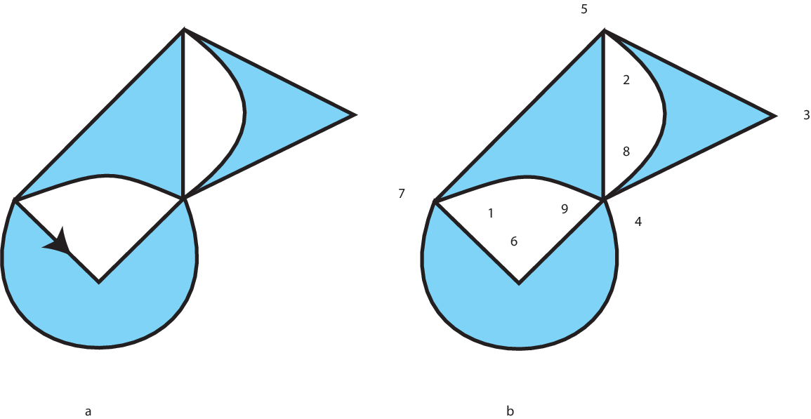
For example, on the left side of Figure 1, marked as “a”, we give a rooted hypermap in the sphere, in which there are three faces of each colour (the black faces have shaded interiors).

Let $M^{g}_{\alpha,\beta}$ denote the number of rooted hypermaps in an orientable surface of genus $g$, with vertex-degrees specified by the parts of the partition $\alpha$, and hyperedge (black face) degrees specified by the parts of $\beta$. It is well-known (see, e.g., [JV1], [JV2], [LZ], [T]) that

Indeed, this explains the use of the term $m$-hypermap numbers for $N^{(g,m)}_{\alpha,\beta}$ (which is simply a rescaling of $c^{(g,m)}_{\alpha,\beta}$, via (31)). The $(d-1)!:1$ correspondence implicit in (36) is described as follows: Label the corners of the white faces $1,\ldots,d$ so that $1$ is assigned to the corner on the counterclockwise side of the root edge, as encountered when moving around the tail vertex. The remaining $d-1$ labels may be placed arbitrarily, to give the factor $(d-1)!$. From this labelled hypermap, we obtain three permutations in $\mathfrak{S}_{d}$: $\sigma$, $\gamma$ and $\pi$. Each disjoint cycle of $\sigma$ gives the labels encountered when moving around a vertex in a counterclockwise direction. Each disjoint cycle of $\pi$ gives the labels encountered when traversing the interior boundary of a hyperface in a counterclockwise direction. Define the label of a black corner (i.e., a corner of a hyperedge) to be the label of the white corner that is encountered in the clockwise direction when moving around their common vertex. Based on this labelling convention, each disjoint cycle of $\gamma$ gives the labels encountered when traversing the interior boundary of a hyperedge in a counterclockwise direction. Given a rooted hypermap counted by $M^{g}_{\alpha,\beta}$, it is clear by construction that $\sigma\in\mathcal{C}_{\alpha}$ and $\gamma\in\mathcal{C}_{\beta}$, and that $\sigma\gamma\pi=\iota$. Moreover, $\langle\sigma,\gamma,\pi\rangle$ acts transitively on $\{1,\ldots,d\}$, because the underlying graph is connected. This is clearly reversible, and specifies the required $(d-1)!:1$ correspondence.

For example, on the right side of Figure 1, marked as “b”, is one of the labellings of the hypermap given on the left side. For this example, we obtain

and it is easy to verify that, in this case, we have $\sigma\gamma\pi=\iota$.

It is instructive to consider the genus $g$ in (23), which gives the genus for the corresponding branched cover. In terms of the hypermap in the present case (with $m=1$), condition (23) gives

References

- [BGR] E.A.Bender, Z. Gao and L.B.Richmond, Calculating the asymptotic coefficients using a new recursion for rooted cubic maps, preprint 2008.
- [BMS] M. Bousquet-Mélou and G. Schaeffer, Enumeration of planar constellations, Adv. Appl. Math. 24 (2000), 337 – 368.
- [G] Zhi-Cheng Gao, The number of rooted triangular maps on a surface, J. Comb. Theory (B) 52 (1991), 236 – 249.
- [GJ1] I.P. Goulden and D.M. Jackson, Combinatorial Enumeration, John Wiley and Sons, New York, 1983 (reprinted by Dover, 2004).
- [GJ2] I.P. Goulden and D.M. Jackson, Transitive factorizations into transpositions and holomorphic mappings on the sphere, Proc. Amer. Math. Soc. 125 (1997), 51 – 60.
- [GS] I.P. Goulden and Luis. G. Serrano, A Simple Recurrence for Covers of the Sphere With Branch Points of Arbitrary Ramification, Annals Comb. 10 (2006), 431 – 441.
- [GJV] I.P. Goulden, D.M. Jackson and R. Vakil, Towards the geometry of double Hurwitz numbers, Advances Math. 198 (2005), 43 –92.
- [H] A. Hurwitz, Ueber Riemann’sche Flächen mit gegebenen Verzweigungspunkten, Math. Ann. 39 (1891), 1 – 60.
- [J] D.M. Jackson, On an integral representation for the genus series for -cell embeddings, Trans. Amer. Math. Soc. 344 (1994), 755 – 772.
- [JV1] D.M. Jackson, T. Visentin, A character theoretic approach to embeddings of rooted maps in an orientable surface of given genus, Trans. Amer. Math. Soc. 322 (1990), 343 – 363.
- [JV2] D.M. Jackson, T. Visentin, Character theory and rooted maps in an orientable surface of given genus: Face-colored maps, Trans. Amer. Math. Soc. 322 (1990), 365 – 376.
- [JV3] D.M. Jackson and T.I. Visentin, An atlas of the smaller maps in orientable and non-orientable surfaces, CRC Press, 2001.
- [Ka] M. Kazarian, KP hierarchy for Hodge integrals, preprint 2007.
- [KL] M. Kazarian and S. Lando, An algebro-geometric proof of Witten’s conjecture, preprint 2005, math.AG/0601760.
- [Ko] M. Kontsevich, Intersection theory on the moduli space of curves and the matrix Airy function, Comm. Math. Phys. 147 (1992), 1 – 23.
- [LZ] S.K. Lando and A.K. Zvonkin, Graphs on Surfaces and Their Applications, Encyclopaedia of Math. Sci., vol 141, Springer-Verlag, Berlin, 2004.
- [MJD] T. Miwa, M. Jimbo and E. Date, Solitons: Differential Equations, Symmetries and Infinite Dimensional Algebras, Cambridge University Press, Cambridge, 2000.
- [Ok] A. Okounkov, Toda equations for Hurwitz numbers, Math. Res. Letters 7 (2000), 447 –453.
- [Or] A. Orlov, Hypergeometric functions as infinite-soliton Tau functions, Theoretical Math. Phys., 146 (2006), 183 –206.
- [OS] A. Orlov and D.M. Shcherbin, Hypergeometric solutions of soliton equations, Theoretical Math. Phys., 128 (2001), 906 – 926.
- [P] R. Pandharipande, The Toda equations and the Gromov-Witten theory of the Riemann sphere, Lett. Math. Phys. 53 (2000), 59 – 74.
- [S] R.P. Stanley, Enumerative Combinatorics, Volume 2, Cambridge University Press, 1999.
- [T] W.T. Tutte, Graph Theory, Encyclopedia of Math. and Applns. 21, Addison-Wesley, London, 1984.
- [W] E. Witten, Two dimensional gravity and intersection theory on moduli space, Survey Diff. Geom. 1 (1991), 243 – 310.