BCS superconductivity of Dirac electrons in graphene layers

– We assume the energy spectrum in graphene in the form

The upper or lower sign refers to the conduction or valence band, respectively; $E_{F0}$ is the Fermi energy without doping when the Dirac point lies at the Fermi level. If the Fermi energy is shifted by some amount $\mu$ due to doping, $E_{F}=E_{F0}+\mu$, (see Fig. 1) the energy measured from the Fermi level is

The group velocity is $d\xi_{\bf p}/d{\bf p}=\pm v{\bf n}$ where ${\bf n}={\bf p}/p$. For electron doping, $\mu>0$, we have for $\xi_{\bf p}<0$

Similar relations take place in the case of hole doping, $\mu=-|\mu|$, as well.

– We use the standard BCS theory and assume an s-wave pairing interaction $V_{p}=-|V_{p}|$, where $|V_{p}|\sim|V|a^{2}$ is the Fourier transform of the pairing potential, $V$ is the energy amplitude, and $a$ is the range of interaction. We do not consider here the nature of pairing interaction, but refer the reader to Refs. [8, 11, 12, 9] where various possible mechanisms are discussed. The coupling constant $\lambda$ is introduced through the equation

Here $\xi_{m}$ determines the interval where attractive interaction is present. In what follows we consider the case of low doping when $|\mu|<\xi_{m}$.

The BCS gap equation in a spatially uniform case is

where the energy of excitations is $E_{\bf p}=\sqrt{\xi_{\bf p}^{2}+\Delta^{2}}$, the phase volume is $d^{2}p=p\,dp\,d\phi$, where $\phi$ is the azimuthal angle of ${\bf n}$, and $n(E_{\bf p})$ is the equilibrium Fermi distribution of quasiparticles with energies $E_{\bf p}$. For zero temperature $1-2n(E)={\rm sign}(E)$. With help of Eq. (1), the BCS gap equation becomes

for both electron and hole doping.

For zero doping $\mu=0$ we have

Nonzero $\Delta$ is possible only for the strong-coupling limit $\lambda>1$ [10]. However, Eq. (3) shows that, for a finite doping, a finite $\Delta_{0}$ exists even in the weak coupling limit $\lambda<1$. In the case of low doping level when $\Delta_{0}$ is small, Eq. (3) gives the gap in a BCS form

with the prefactor determined by the doping level $|\mu|$ rather than by the range of interaction.

– For a finite temperature Eq. (2) yields the gap equation

For $T\rightarrow 0$ we return to Eq. (3). Equation (6) leads to the equation for the critical temperature

where

where $F(x)>0$. The critical temperature found from Eq. (7) is plotted in Fig. 2.

For $\mu=0$ the critical temperature satisfies $\Phi\left(\xi_{m}/2T_{c};\lambda\right)=0$, i.e.,

This equation has a solution only for interaction strength above the quantum critical point, $\lambda>1$ (see Fig. 2). If $\lambda\rightarrow 1$ we have $T_{c}=\xi_{m}(\lambda-1)/2\ln 2$ which vanishes at $\lambda=1$. Comparing this with Eq. (4) we find $\Delta_{0}=T_{c}2\ln 2$. In the other limit $\lambda\gg 1$ we find $T_{c}=\xi_{m}\lambda/4$ and $\Delta_{0}=2T_{c}$. These results agree with Ref.[10] where only undoped case was considered.

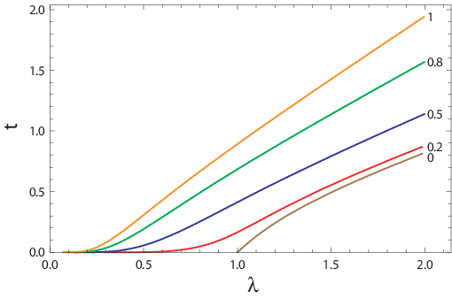
However, for any low but finite doping level the critical temperature is finite. Consider weak coupling limit $\lambda\ll 1$ where we expect $T_{c}\ll\mu$. Indeed, the l.h.s. of Eq. (7) is $\Phi(y;\lambda)=y(\lambda^{-1}-1)+\ln 2$ already for $T_{c}\ll\xi_{m}$. On the other hand, for $x\gg 1$ the r.h.s. of Eq. (7) is

where $\gamma=e^{C}=1.78$ and $C=0.5772$ is the Euler constant. This yields

resulting in the BCS relation $\Delta_{0}=(\pi/\gamma)T_{c}=1.76T_{c}$.

Consider the vicinity of the quantum critical point $\mu=0$ and $\lambda=1$. On the weak coupling side $\lambda<1$, the critical temperature is given by Eq. (10) which is exact provided $T_{c}\ll|\mu|$, i.e., for $1-\lambda\gg|\mu|/\xi_{m}$. For $|\mu|/\xi_{m}\sim 1$ and $\lambda\rightarrow 1$, Eq. (10) works also reasonably well. For example, Eq. (10) gives $T_{c}\approx 0.42|\mu|$ for $\lambda=1$. This can be compared to the exact value for $\lambda=1$ which is found from the condition $F(|\mu|/2T_{c})=\ln 2$ resulting in $T_{c}\approx 0.40|\mu|$. In the limit $\mu\ll T_{c}\ll\xi_{m}$ which is more appropriate on the strong-coupling side of the quantum critical point

This holds for $|\mu|/\xi_{m}\ll\lambda-1\ll 1$, but also matches with the exact $T_{c}$ by the order of magnitude when $\lambda\rightarrow 1$.

Therefore we come to the conclusion that a finite $T_{c}$ does always exist for a finite $\mu$. If $\lambda\gtrsim 1$, the critical temperature is close to that determined by Eq. (8) as long as $\mu\ll\xi_{m}$. If $\lambda\lesssim 1$ we essentially have Eq. (10).

– Let us assume a homogeneous flow of the condensate: $\Delta=|\Delta|e^{i{\bf k}_{s}{\bf r}}$, where ${\bf k}_{s}=\nabla\chi$ is a constant gradient of the order-parameter phase. In the presence of magnetic field, ${\bf k}_{s}=\nabla\chi-(2e/\hbar c){\bf A}$. Consider the state described by the particle-like and hole-like Bogoliubov-de Gennes wave functions

where ${\bf p}_{\pm}={\bf p}\pm\hbar{\bf k}_{s}/2$,

$E_{D}=(d\xi_{p}/d{\bf p})\hbar{\bf k}_{s}/2$ is the Doppler energy, and

are the coherence factors. The standard expression for the current is

Expanding Eq. (11) for small $E_{D}\ll\Delta,T$ and making shift in the momentum variable we find for the two-dimensional current density in the linear response regime

This yields the current

where $\Lambda$ is the characteristic energy. For zero temperature we have

In contrast to the usual superconductors the supercurrent density is not proportional to the total electron density, being drastically affected by the presence of the Dirac point. In particular, for weak coupling limit, $|\Delta|\ll\mu$, the current ${\bf j}=e\mu{\bf k}_{s}/4\pi\hbar$ is proportional to $|\mu|\propto\sqrt{n}$, where $n$ is the density of free carriers provided by doping. Near the quantum critical point when $T\ll\xi_{m}$, the current is determined by the superconducting gap itself. Indeed, for zero doping, Eq. (11) yields

For low temperatures, $T\ll|\Delta|$, we have ${\bf j}=e|\Delta|{\bf k}_{s}/4\pi\hbar$. Close to $T_{c}$, where $|\Delta|\ll T_{c}$, the current assumes the Ginzburg-Landau form ${\bf j}=e|\Delta|^{2}{\bf k}_{s}/8\pi\hbar T_{c}$.

– As usual the critical fields are determined by two spatial scales: the coherence length $\xi_{0}$ and the London penetration depth $\lambda_{L}$. At zero temperature the London penetration length for a graphene layer with thickness $d$ is

It diverges near the quantum critical point $\lambda\rightarrow 1$, $\mu\rightarrow 0$. For the undoped case the London length is $\lambda_{L}=(\Phi_{0}/\pi)\sqrt{d/2\Delta}$, where $\Phi_{0}=\pi\hbar c/e$ is the magnetic-flux quantum. Close to the critical temperature the London length, $\lambda_{L}=(\Phi_{0}/\pi\Delta)\sqrt{T_{c}d}$, is inversely proportional $\sqrt{T_{c}-T}$ as in conventional superconductors. The coherence length has a standard form: $\xi_{0}\sim\hbar v_{F}/\Delta$. Thus the Ginzburg-Landau parameter $\kappa=\lambda_{L}/\xi_{0}$, which characterizes the type of superconductivity, does not depend on the temperature near $T_{c}$ as is the case in conventional superconductors:

For typical values $v_{F}=10^{8}$ cm/s, $d=10^{-7}$ cm, and for $T_{c}\sim 1$ K, the Ginzburg-Landau parameter is on the border between the two types, $\kappa\sim 1$. Therefore, close to the quantum critical point where $T_{c}\to 0$ the superconductivity definitely becomes of type I.

To summarize, we have calculated the critical temperature, the superconducting gap, and the supercurrent as functions of the doping level and of the interaction strength for an s-wave pairing within the BCS model. The superconducting transition in the undoped graphene has a quantum critical point with respect to the interaction strength, which disappears for any finite doping level such that a finite critical temperature exists for any weak pairing interaction. The amplitude of the supercurrent is drastically affected by the presence of the Dirac point, which leads to non-trivial behavior of the characteristic length scales (penetration depth and coherence length) determining critical magnetic fields.