1Introduction

SI-HEP-2007-21

16.04.2008, revised 10.07.2008

Is there a non-Standard-Model contribution
in non-leptonic $b\to s$ decays?

Thorsten Feldmann, Martin Jung, Thomas Mannel

Universität Siegen, Fachbereich Physik
D-57068 Siegen, Germany.

Precision measurements of branching fractions and CP asymmetries in non-leptonic $b\to s$ decays reveal certain “puzzles” when compared with Standard Model expectations based on a global fit of the CKM triangle and general theoretical expectations. Without reference to a particular model, we investigate to what extent the (small) discrepancies observed in $B\to J/\psi K$ , $B\to\phi K$ and $B\to K\pi$ may constrain new physics in $b\to sq\bar{q}$ operators. In particular, we compare on a quantitative level the relative impact of different quark flavours $q=c,s,u,d$ .

1 Introduction

Exclusive non-leptonic $B$ meson decays remain a challenge to theory. While semi-leptonic $B$ decays are well described within the heavy-mass expansion and allow for a rather precise determination of the CKM matrix elements $|V_{cb}|$ and $|V_{ub}|$ , exclusive non-leptonic decays still cannot be described at a similar level of precision. The methods that have been proposed so far are based on the flavour symmetries of QCD [1, 2, 3, 4, 5, 6, 7], the factorization of QCD dynamics in hadronic matrix elements [8, 9, 10, 11, 12], or combinations thereof [13, 14, 15]. The level of precision that one expects from these methods is typically of the order of tens of percent, and thus – except for a few “gold-plated” observables – it will in general be hard to pin down an effect from new physics (NP) in these decays. Still, from the experimental side, the B-factories have collected sufficient information on decay widths and CP asymmetries to allow for global fits of the Standard Model (SM) parameters, in particular of the elements of the Cabibbo-Kobayashi-Maskawa (CKM) matrix [16, 17].

The agreement between the standard theory and experimental data is overall satisfactory, however, in some cases small tensions appear. In the present paper we focus on the $|\Delta B|=|\Delta S|=1$ decay modes $B\to J/\Psi K$ , $B\to\phi K$ and $B\to K\pi$ , which enter some of the present-day “puzzles”. Taking the experimental results at face value, we pursue the hypothesis that these “discrepancies” with the SM calculations are due to non-standard effects [18]. We adopt a model-independent parameterization in terms of isospin amplitudes, where we allow for additional contributions from generic NP operators. The moduli, as well as the strong phases of the additional terms are then fitted to experimental data on decay widths and CP asymmetries. The new weak phase will generally remain undetermined due to reparameterization invariance, as long as we do not attempt to fix the hadronic SM matrix elements. In the case of $B\to K\pi$ decays we make use of additional theoretical input from the QCD-improved factorization approach (QCDF) [9].

Our paper is organized as follows: In the next section we point out the tensions of the SM fit with present data, and give arguments for the way we are going to re-fit the experimental data including generic NP contributions. In the following section we discuss the results of the fits for the individual decay modes and present our conclusions in Section 4.

2 Phenomenology

Refer to caption — Figure 1: Global fit to CKM parameters from $\Delta m_{d}$ , $\Delta m_{s}$ and $|V_{ub}/V_{cb}|_{\rm excl.+incl.}$ . Left: Confidence levels in the $\bar{\eta}-\bar{\rho}$ plane. Right: Fitted values for CKM parameters, where the first error is treated as Gaussian, and the second error is treated as flat.

quantity	value
$\sin 2\beta$	$0.758^{+0.012}_{-0.021}\pm 0.075$
$\gamma$	$(59.6^{+2.1}_{-2.3}\pm 5.4)^{\circ}$

2.1 Tensions with the Standard Model?

In the following we give a brief discussion of the present situation for the $B$ physics observables that we are going to consider, where the standard model displays some tension with the data:

•

The first point concerns the global fit of the CKM unitarity triangle. Here a small mismatch appears between the value of the CKM angle $\beta$ obtained from the direct measurement of the time-dependent CP asymmetry in $B\to J/\psi K_{S}$ and the indirect determination of the same angle from the mass differences in the neutral $B$ -meson systems, $\Delta m_{d}/\Delta m_{s}$ , in combination with the measurement of $|V_{ub}/V_{cb}|$ from semi-leptonic decays [17, 19, 20, 21, 22, 23]. In fact, using the values from [19], we find for the latter case $\sin 2\beta=0.758^{+0.012}_{-0.021}\pm 0.075_{\rm flat}$ (see Fig. 1), while the direct determination using $B\to J/\Psi K_{S}$ yields $\sin 2\beta=0.678\pm 0.025$ [24]. However, the significance of this effect depends strongly on the estimates of the theoretical uncertainties, e.g. in the determination of $|V_{ub}|$ , and can certainly not be taken as a clear evidence for a non-standard effect.
•

The second puzzle arises from the time-dependent CP asymmetry in modes like $B\to\phi K_{S}$ which in the SM again yields a determination of $\sin 2\beta$ , although with less precision. The value for $\beta$ obtained from fits to several $b\to s\bar{s}s$ penguin modes¹¹ 1 Following the arguments given by HFAG [24], we do not consider the $\sin 2\beta$ value extracted from $B^{0}\to f_{0}K_{S}$ for our discussion, due to the highly non-Gaussian error implied by the BaBar measurement [25]. does not agree with the value from the CP asymmetry in $B\to J/\Psi K_{S}$ [24]. While part of the discrepancy may be due to not well understood hadronic effects, it is at least curious that the bulk of decay modes involving the $b\to s\bar{s}s$ penguin systematically yields a lower value for $\sin 2\beta$ than the one obtained from $B\to J/\Psi K_{S}$ (see also [26]).
•

Finally, the theoretical predictions for $B\to K\pi$ decay widths and CP asymmetries are not always in very good agreement with the data. Within the QCD factorization approach the discrepancy with the data can be brought to an “acceptable” level (except for, perhaps, the differences of CP asymmetries $\Delta A$ , see the discussion in Sec. 3.5.1 below) by assuming particular scenarios within the hadronic parameter space, including undetermined $1/m_{b}$ corrections [27]. On the other hand, analyses based on $SU(3)$ flavour symmetry for hadronic matrix elements typically have found tensions of the order of $(2-3)\,\sigma$ [6, 11, 13, 16, 28, 29, 30, 31], depending on additional assumptions about hadronic matrix elements. It should be noted that the tensions related to the branching fractions have decreased since the inclusion of electromagnetic corrections in the experimental analysis (for a recent update of the discussion see, for instance, [32]).

Let us, for the moment, take these tensions between theoretical expectations and experimental data at face value: Assuming that they are not due to enormous deviations from the factorization approximation to hadronic matrix elements, we may try to localize in which part of the effective weak Hamiltonian we have to look for NP effects.

A first possibility are non-standard contributions in the charged $b\to u$ current which determines $|V_{ub}|$ . However, it is generally believed to be unlikely that these tree-level processes contain sizeable NP effects. Likewise, the theoretical description of QCD dynamics in semi-leptonic decays is fairly well under control, and hence we will not consider this possibility here.

A second explanation could be a non-standard contribution in the mixing phase of the $|\Delta B|=2$ part of the effective Hamiltonian, which shifts the observed $\sin 2\beta$ to smaller values. Such a scenario corresponds to a generalization of Wolfenstein’s “superweak interaction” [33]. Obviously, it cannot explain the differences in the $\sin 2\beta$ measurements from $b\to c\bar{c}s$ and $b\to s\bar{s}s$ modes.

The third scenario, which is the one we are going to expand on in this work, is the possibility to have an additional contribution in the $|\Delta B|=|\Delta S|=1$ part of the effective Hamiltonian. Evidently, the inclusion of such terms can explain the findings in $B\to J/\Psi K_{S}$ and $B\to\phi K_{S}$ , as well as in $B\to K\pi$ . When fitted to experimental data, the values for the NP contributions, relative to the leading hadronic amplitudes in the SM, can be as large as about 30%. If NP is the explanation for the tensions in non-leptonic $b\to s$ transitions, structures beyond minimal-flavour violation (MFV [34, 35, 36]) are favoured, mainly because the deviations in the $B\to\phi K$ CP asymmetries point towards an independent NP phase, but also because the constraints on contributions from different flavours $q$ in $b\to sq\bar{q}$ generally can be rather different in size.

3 Fit of new physics contributions to experimental data

3.1 $|\Delta B|=|\Delta S|=1$ transitions

Using the unitarity of the CKM matrix, the SM operator basis for non-leptonic $b\to s$ transitions can be written as [37]

H_{\rm SM}^{|\Delta B|=|\Delta S|=1}=\frac{G_{F}}{\sqrt{2}}\,V_{cb}V_{cs}^{*}\left(C_{1,2}\,O_{1,2}^{(c)}+\sum_{i\geq 3}C_{i}\,O_{i}\right)+\frac{G_{F}}{\sqrt{2}}\,V_{ub}V_{us}^{*}\left(C_{1,2}\,O_{1,2}^{(u)}+\sum_{i\geq 3}C_{i}\,O_{i}\right)\,,

(1)

where $O_{1,2}^{(q)}$ are the current-current operators, $O_{3-6}$ the strong penguins, $O_{7-10}$ the electroweak penguins, and $C_{7}^{\gamma}$ , $C_{8}^{g}$ the electromagnetic and chromomagnetic operators, respectively. At low energies, the effect of NP in $|\Delta B|=|\Delta S|=1$ transitions will be parameterized by new dimension-six operators. In the following we shall focus on generic four-quark operators of the type $b\to sq\bar{q}$ with $q=(b),c,s,u,d$ , where the Dirac and colour structure will not be specified. In order to quantify the possible size of NP contributions, we will always assume the dominance of one particular flavour structure, and parameterize the corresponding correction to the SM decay amplitudes in a model-independent way.

3.2 Statistical framework

The parameter space for the NP amplitudes is explored using the CKMfitter package [38]. Here the amplitude parameters are treated as fundamental theoretical quantities, and the statistical analysis provides the relative likelihood for a given point in parameter space (corresponding to model-dependent “metrology” in the CKMfitter jargon). Other theoretical parameters, like hadronic uncertainties from SM physics, are treated using the Rfit-scheme, where the corresponding $\chi^{2}$ -contribution is set to zero within a “theoretically acceptable” range, and set to infinity outside. We will sometimes apply the same approach to implement additional theoretical constraints/assumptions on the amplitude parameters, in order to suppress ”unphysical” solutions.

3.3 Analysis of $B\to J/\Psi K$

For $B\to J/\Psi K$ decays the contribution of the second term in the weak effective Hamiltonian (1) is small because of two effects:

•

Cabibbo suppression: $|V_{ub}V_{us}^{*}|/|V_{cb}V_{cs}^{*}|\sim\lambda^{2}\ll 1$
•

Penguin suppression: (i) The operators $O_{1,2}^{(u)}$ do not contain charm quarks, and the hadronic matrix elements $\langle J/\psi K|O_{1,2}^{(u)}|B\rangle$ are suppressed. (ii) The coefficients of the loop-induced penguin operators $C_{i\geq 3}$ are small with respect to the tree coefficients $C_{1,2}$ .

Furthermore, the electroweak penguin operators can be neglected compared to the strong penguin operators. Consequently, in the SM the $B\to J/\psi K$ decay amplitude is expected to be completely dominated by

{\cal A}_{0}(\bar{B}\to J/\psi\bar{K})=\frac{G_{F}}{\sqrt{2}}\,V_{cb}V_{cs}^{*}\,\langle J/\psi\bar{K}|C_{1,2}\,O_{1,2}^{(c)}+\sum_{i=3}^{6}C_{i}O_{i}^{(c)}|\bar{B}\rangle

(2)

where $\bar{B}=\{\bar{B}^{0}_{d},\,B^{-}\}$ , and we projected out the leading $[\bar{s}b\bar{c}c]$ component in every operator, $O_{i}\to O_{i}^{(c)}$ . In particular, the amplitude is dominated by a single weak phase, and consequently the time-dependent CP asymmetry in $B^{0}\to J/\psi K_{S}$ is completely determined by the $B^{0}-\bar{B}^{0}$ mixing amplitude, involving the CKM angle $\beta$ . Corrections from the sub-leading operators have been estimated by perturbative methods at the $b$ -quark scale,²² 2 The authors of [39] only considered the effect of $O_{1,2}^{u}$ . In [40] important contributions from $C_{3-6}$ have been included as well. and found to give effects of the order of $10^{-3}$ , only [39, 40]. Long-distance penguin contributions have been estimated on the basis of experimental data to be not larger than $10^{-2}$ [41].

$\eta_{\rm CP}\,S_{J/\psi K_{S}}$	$-0.678\pm 0.026$
$C_{J/\psi K_{S}}$	$\phantom{+}0.012\pm 0.020$
$A_{\rm CP}(J/\psi K^{-})$	$\phantom{+}0.015\pm 0.017$
$\Gamma(B^{-}\to J/\Psi K^{-})$	$(6.13\pm 0.22)\cdot 10^{-4}\,{\rm ps}^{-1}$
$\Gamma(\bar{B}^{0}\to J/\Psi\bar{K}^{0})$	$(5.71\pm 0.22)\cdot 10^{-4}\,{\rm ps}^{-1}$

Table 1: Partial widths [21] and CP asymmetries [24] for

B\to J/\Psi K

Furthermore, the dominating operators in the SM decay amplitude conserve strong isospin ( $\Delta I=0$ ), and therefore do not induce differences between the charged and neutral $B$ decays into $J/\psi K$ . The present experimental data is summarized in Table 1. We note that the central value for $S_{J/\psi K_{S}}$ differs from the indirect determination for $\sin 2\beta$ in Fig. 1, but the two values are consistent within the errors. The discrepancy becomes slightly more pronounced, if one takes into account the inclusive measurement for $|V_{ub}|$ only, which gives

\sin 2\beta=0.821^{+0.024}_{-0.046}\pm 0.068_{\rm flat}\qquad\mbox{(using $|V_{ub}|_{\rm incl.}$ from \cite[cite]{[\@@bibref{}{Lacker:2007me}{}{}]}).}

Similarly, the central values for the observed isospin-breaking in the CP asymmetries ( $C_{J/\psi K_{S}}$ vs. $-A_{\rm CP}(J/\psi K^{-})$ ) and partial widths differ from zero.

Allowing for generic NP contributions with one weak phase $\theta_{W}$ , the amplitudes can be written as

	$\displaystyle{\cal A}(B^{-}\to J/\psi K^{-})$	$\displaystyle=$	$\displaystyle{\cal A}_{0}(\bar{B}\to J/\psi K)\left[1+r_{0}\,e^{i\theta_{W}}e^{i\phi_{0}}-r_{1}\,e^{i\theta_{W}}e^{i\phi_{1}}\right]\,,$		(3)
	$\displaystyle{\cal A}(\bar{B}_{d}\to J/\psi\bar{K}^{0})$	$\displaystyle=$	$\displaystyle{\cal A}_{0}(\bar{B}\to J/\psi K)\left[1+r_{0}\,e^{i\theta_{W}}e^{i\phi_{0}}+r_{1}\,e^{i\theta_{W}}e^{i\phi_{1}}\right]\,,$		(4)

where we have separated the contributions to transitions with $\Delta I=0$ (i.e. tree-level matrix elements with $b\to sc\bar{c}$ operators or long-distance strong penguins with $b\to s(u\bar{u}+d\bar{d})$ or $b\to ss\bar{s}$ operators) and $\Delta I=1$ (annihilation topologies with $b\to su\bar{u}$ or $b\to sd\bar{d}$ ). We introduced the absolute values $r_{0}$ , $r_{1}$ and strong phases $\phi_{0}$ , $\phi_{1}$ for the hadronic matrix elements associated with the corresponding NP operators, relative to the leading SM amplitude.

3.3.1 Fit with $\Delta I=0$ only (new physics in $b\to sc\bar{c}$ )

Among the $\Delta I=0$ and $\Delta I=1$ operators we expect the $b\to sc\bar{c}$ term to give the dominating contributions to $B\to J/\psi K$ decays, because it has (unsuppressed) tree-level matrix elements with the hadronic final state. Therefore, let us first assume that $b\to sc\bar{c}$ gives the only relevant NP contribution in (4) which amounts to setting $r_{1}$ to zero, while $r_{0}$ should be of the order $m_{W}^{2}/\Lambda_{\rm NP}^{2}$ . Then, the isospin breaking between charged and neutral $B$ decays is not affected, and should not be part of the fit. We are thus left with the time-dependent CP asymmetries, defined as in [16]

A_{\rm CP}(f,t):=\frac{{\rm BR}[\bar{B}^{0}\to f](t)-{\rm BR}[B^{0}\to\bar{f}](t)}{{\rm BR}[\bar{B}^{0}\to f](t)+{\rm BR}[B^{0}\to\bar{f}](t)}:=-C_{f}\cos(\Delta m\,t)+S_{f}\sin(\Delta m\,t)

(5)

and the direct CP asymmetry $A_{\rm CP}^{\rm dir}(B^{-}\to J/\psi K^{-})=-C_{J/\psi K_{S}}$ . Including the contribution from $r_{0}$ in (4), we obtain

$\displaystyle C_{J/\psi K_{S}}$	$\displaystyle=$	$\displaystyle-A_{\rm CP}^{\rm dir}(B^{-}\to J/\psi K^{-})$	(6)
	$\displaystyle=$	$\displaystyle\frac{2r_{0}\,\sin\phi_{0}\,\sin\theta_{W}}{1+2r_{0}\,\cos\phi_{0}\,\cos\theta_{W}+r_{0}^{2}}\,,$	(6)
$\displaystyle\eta_{\rm CP}\,S_{J/\psi K_{S}}$	$\displaystyle=$	$\displaystyle-\sin(2\beta)+\frac{2r_{0}\,\sin\theta_{W}\left(\cos(2\beta)\,\cos\phi_{0}+r_{0}\,\cos(2\beta-\theta_{W})\right)}{1+2r_{0}\,\cos\phi_{0}\,\cos\theta_{W}+r_{0}^{2}}\,.$	(7)

We expect the NP amplitudes to provide small corrections to the SM, $0\leq r_{0}\ll 1$ , and thus to first approximation we have

	$\displaystyle C_{J/\psi K_{S}}$	$\displaystyle\simeq$	$\displaystyle 2r_{0}\,\sin\theta_{W}\,\sin\phi_{0}\,,$
	$\displaystyle\eta_{\rm CP}\,S_{J/\psi K_{S}}+\sin(2\beta)$	$\displaystyle\simeq$	$\displaystyle 2r_{0}\,\sin\theta_{W}\,\cos\phi_{0}\,\cos(2\beta)\,.$		(8)

From this we read off the interesting parameter combinations

|r_{0}\sin\theta_{W}|\simeq\frac{\sqrt{(\eta_{\rm CP}\,S_{J/\psi K_{S}}+\sin 2\beta)^{2}+(C_{J/\psi K_{S}}\,\cos 2\beta)^{2}}}{2\cos 2\beta}\,,

(9)

determining the overall size of the deviations of $C$ from 0, and of $S$ from $\sin 2\beta$ , and

\tan\phi_{0}\simeq\frac{C_{J/\psi K_{S}}\,\cos 2\beta}{\eta_{\rm CP}\,S_{J/\psi K_{S}}+\sin 2\beta}\,,

(10)

determining the relative size of the two effects.

Notice that from the CP asymmetries alone we cannot draw any conclusion about the value of the NP phase $\theta_{W}$ . This is a consequence of a reparameterization invariance (see e.g. [42]) which leaves the decay amplitudes for the neutral $B$ decays in (4), as well as the branching fraction and the direct CP asymmetry for the charged $B$ decays invariant,

	$\displaystyle{\cal A}_{0}^{\prime}={\cal A}_{0}\left(1+\xi\,(r_{0}\,e^{i\phi_{0}}+r_{1}\,e^{i\phi_{1}})\right)\,,$
	$\displaystyle\cos\theta_{W}^{\prime}=\frac{\cos\theta_{W}-\xi}{\sqrt{1-2\,\xi\,\cos\theta_{W}+\xi^{2}}}\,,\qquad\sin\theta_{W}^{\prime}=\frac{\sin\theta_{W}}{\sqrt{1-2\,\xi\,\cos\theta_{W}+\xi^{2}}}\,,$		(11)

and similar transformations for the amplitude parameters $r_{0,1}$ and $\phi_{0,1}$ , where the parameter $\xi$ (and therefore also the values for $r_{0,1}$ , $\phi_{0,1}$ and $\theta_{W}$ ) is arbitrary as long as the hadronic matrix element ${\cal A}_{0}$ for the leading SM contribution is not given explicitly. In particular, for $r_{1}=0$ , $r_{0}\ll 1$ and small reparameterizations $\xi\ll 1$ , we approximately have

	$\displaystyle r_{0}$	$\displaystyle\to$	$\displaystyle r_{0}\left(1-\xi\,\cos\theta_{W}+{\cal O}(\xi^{2})\right)\,,\qquad\phi_{0}\to\phi_{0}\left(1+{\cal O}(\xi^{2})\right)\,,$		(12)
	$\displaystyle\sin\theta_{W}$	$\displaystyle\to$	$\displaystyle\sin\theta_{W}\left(1+\xi\,\cos\theta_{W}+{\cal O}(\xi^{2})\right)\,,$		(13)

which explicitly shows the reparameterization invariance of (8).

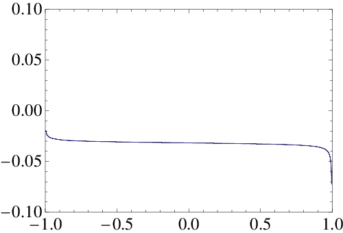
The reparameterization invariance is illustrated in Fig. 2, where as an example we consider the fit result for a $\Delta I=0$ NP contribution with $\theta_{W}=\pi-\gamma_{\rm SM}$ found in the last row of Table 2 below, and apply the reparameterizations in (11) to generate the equivalent solutions for other values of $\theta_{W}$ . In particular, we verify that the combinations $r_{0}\,\sin\theta_{W}$ and $\tan\phi_{0}$ are approximately reparameterization-invariant, except for $\theta_{W}$ near zero or $\pi$ .

As a consequence of the reparameterization invariance, the fit to the experimental data will generally allow for ”unphysical” solutions, where the strong and weak phases are tuned in such a way that the absolute size of the NP contribution $r_{0}$ can be unreasonably large. In order to suppress such effects, we implement additional constraints: (i) For small NP contributions, the fit should not depend on the parameter combination $|r_{0}\,\cos\theta_{W}|$ ; constraining $|r_{0}\,\cos\theta_{W}|<0.4$ should therefore only affect the unphysical solutions. (ii) If the phase $\theta_{W}$ of the NP operator is close to the SM one, we do not expect to be sensitive to NP in CP asymmetries in any case; we may therefore concentrate on $30^{\circ}\leq\theta_{W}\leq 150^{\circ}$ . (iii) For $\theta_{W}=\pi-\gamma_{\rm SM}$ our fit can also be interpreted as a determination of the size of sub-leading SM contributions from Cabibbo- and penguin-suppressed amplitudes, which possibly may have been underestimated in [39, 40]. In this case, one could also include the information from $B\to J/\psi\pi$ decays to further constrain the hadronic parameters, using $SU(3)$ flavour symmetry [41], and correcting for the different relative CKM factors. Considering the CP asymmetries in $B\to J/\psi\pi$ alone, we find that the constraints on $r_{0}\,e^{i\delta_{0}}$ are less restrictive than and consistent with the $B\to J/\psi K$ case. The ratio of branching fractions in $B\to J/\psi\pi$ and $B\to J/\psi K$ further constrains $r_{0}$ [41]. However, we find that this ratio essentially depends on the combination

\displaystyle\frac{1}{2}\,\frac{\Gamma[B^{0}\to J/\psi K^{0}]}{\Gamma[B^{0}\to J/\psi\pi^{0}]}

\displaystyle\approx\frac{\lambda^{2}}{R_{SU(3)}^{2}\lambda^{4}+r_{0}^{2}}\,,

(14)

and thus the constraints on $r_{0}$ are highly correlated with the assumptions on the $SU(3)$ breaking parameter $R_{SU(3)}$ for the ratio of the leading $B\to J/\psi\pi$ and $B\to J/\psi K$ amplitudes. As this ratio cannot be estimated in a model-independent way at present, we refrain from a detailed quantitative analysis. However, it should be mentioned that for $R_{SU(3)}\approx 1$ , smaller values for $r_{0}$ are favoured.

Using the experimental values for $C_{J/\psi K_{S}}$ , $S_{J/\psi K_{S}}$ , and $A_{\rm CP}^{\rm dir}(B^{-}\to J/\psi K^{-})$ , together with the value for $\sin 2\beta$ from the indirect determination in Fig. 1, we fit the preferred ranges for the NP parameters – applying the different constraints as discussed above – as shown in Table 2 and Fig. 3.

Scenario			$\|r_{0}\,\sin\theta_{W}\|$	$\tan\phi_{0}$
excl.+incl.	$\theta_{W}$ free	$\|r_{0}\cos\theta_{W}\|\leq 0.4$	[0 to 0.23]	unconstrained
	$30^{\circ}\leq\theta_{W}\leq 150^{\circ}$	$\|r_{0}\cos\theta_{W}\|$ free	[0 to 0.19]	unconstrained
	$30^{\circ}\leq\theta_{W}\leq 150^{\circ}$	$\|r_{0}\cos\theta_{W}\|\leq 0.4$	[0 to 0.19]	unconstrained
	$\theta_{W}=\pi-\gamma_{\rm SM}$	$\|r_{0}\cos\theta_{W}\|$ free	[0 to 0.13]	unconstrained
incl.	$\theta_{W}$ free	$\|r_{0}\cos\theta_{W}\|\leq 0.4$	[0.02 to 0.34]	[-0.41 to 0.18]
	$30^{\circ}\leq\theta_{W}\leq 150^{\circ}$	$\|r_{0}\cos\theta_{W}\|$ free	[0.03 to 0.33]	[-0.26 to 0.12]
	$30^{\circ}\leq\theta_{W}\leq 150^{\circ}$	$\|r_{0}\cos\theta_{W}\|\leq 0.4$	[0.03 to 0.33]	[-0.26 to 0.12]
	$\theta_{W}=\pi-\gamma_{\rm SM}$	$\|r_{0}\cos\theta_{W}\|$ free	[0.03 to 0.19]	[-0.24 to 0.11]

Table 2: Fit to direct and mixing-induced CP asymmetries in

B\to J/\psi K

, using the indirect determination of

\sin 2\beta

and including the

\Delta I=0

NP contribution

r_{0}

, only. We show the

1\sigma

confidence level for the two relevant parameter combinations

|r_{0}\sin\theta_{W}|

and

\phi_{0}

, using different additional constraints to suppress ”unphysical” solutions (see text). The upper half of the table corresponds to using the

\sin 2\beta

value from the indirect fit with

|V_{ub}|_{\rm excl.+incl.}

in Fig. 1. In the lower half, only

|V_{ub}|_{\rm incl.}

from [19] is used.

Since the value for $|V_{ub}|$ from the average of inclusive and exclusive decays is close to its indirect determination from $\sin 2\beta$ , the fitted range for $r_{0}\,\sin\theta_{W}$ in this case is consistent with zero, and the related strong phase $\phi_{0}$ is unconstrained. Still, for sufficiently small strong phases, NP contributions of the order 20% are not excluded either. On the other hand, taking into account the inclusive value of $|V_{ub}|$ (with its small tension with $\sin 2\beta$ ) only, the fit prefers non-zero values for $r_{0}\,\sin\theta_{W}$ of the order 5-30% and relatively small strong phases $\phi_{0}$ . (Notice that small strong phases are generally expected within the QCD factorization approach to hadronic matrix elements in the heavy-quark limit [8].) Compared to the estimate of SM corrections in [39, 40], the typical order of magnitude for $r_{0}$ is thus significantly larger. Although the present experimental situation is not conclusive, our analysis shows that an improvement of the experimental precision for $B\to J/\psi K$ observables or of the theoretical precision in the $|V_{ub}/V_{cb}|$ determination may still lead to interesting conclusions.

3.3.2 Fit with $\Delta I=0,1$ (new physics in $b\to su\bar{u}$ or $b\to sd\bar{d}$ )

New physics contributions to either $b\to su\bar{u}$ or $b\to sd\bar{d}$ may lead to isospin asymmetries between charged and neutral $B\to J/\psi K$ decay rates and CP asymmetries. In this case we may fit (4) with both $r_{0}\neq 0$ and $r_{1}\neq 0$ , and consider the observables in Fig. 3 together with the (CP-averaged) isospin breaking in the decay rates [21]

\displaystyle A_{I}(B\to J/\psi K)=\frac{\Gamma[B_{d}\to J/\psi K_{0}]-\Gamma[B^{\pm}\to J/\psi K^{\pm}]}{\Gamma[B_{d}\to J/\psi K_{0}]+\Gamma[B^{\pm}\to J/\psi K^{\pm}]}

\displaystyle=

\displaystyle-0.035\pm 0.026\,.

(15)

For small values of $r_{0}$ and $r_{1}$ , following [43], we have the approximate relations

$\displaystyle\eta_{\rm CP}\,S+\sin 2\beta$	$\displaystyle\simeq$	$\displaystyle\phantom{-}2\left(r_{0}\,\cos\phi_{0}+r_{1}\,\cos\phi_{1}\right)\sin\theta_{W}\,\cos 2\beta\,,$	(16)
$\displaystyle A_{\rm CP}^{\rm avg}$	$\displaystyle\simeq$	$\displaystyle-2\,r_{0}\,\sin\phi_{0}\,\sin\theta_{W}\,,$	(17)
$\displaystyle\Delta A_{\rm CP}$	$\displaystyle\simeq$	$\displaystyle-2\,r_{1}\,\sin\phi_{1}\,\sin\theta_{W}\,,$	(18)
$\displaystyle A_{I}$	$\displaystyle\simeq$	$\displaystyle\phantom{-}2\,r_{1}\,\cos\phi_{1}\,\cos\theta_{W}\,.$	(19)

They are manifestly invariant under the approximate reparameterizations, following from (11) in the limit $\xi={\cal O}(r_{0,1})\ll 1$ ,

$\displaystyle\sin\theta_{W}$	$\displaystyle\to$	$\displaystyle\sin\theta_{W}\left(1+\xi\,\cos\theta_{W}+{\cal O}(\xi^{2})\right)\,,$	(20)
$\displaystyle\cos\theta_{W}$	$\displaystyle\to$	$\displaystyle\cos\theta_{W}-\xi\,\sin^{2}\theta_{W}+{\cal O}(\xi^{2})\,,$	(21)
$\displaystyle r_{0}\,\cos\phi_{0}+r_{1}\,\cos\phi_{1}$	$\displaystyle\to$	$\displaystyle(r_{0}\,\cos\phi_{0}+r_{1}\,\cos\phi_{1})\left(1-\xi\,\cos\theta_{W}+{\cal O}(\xi^{2})\right)\,,$	(22)
$\displaystyle r_{1}\,\cos\phi_{1}$	$\displaystyle\to$	$\displaystyle r_{1}\,\cos\phi_{1}\left(1+\xi\,\sin\theta_{W}\,\tan\theta_{W}+{\cal O}(\xi^{2})\right)\,,$	(23)
$\displaystyle r_{0,1}\,\sin\phi_{0,1}$	$\displaystyle\to$	$\displaystyle r_{0,1}\,\sin\phi_{0,1}\left(1-\xi\,\cos\theta_{W}+{\cal O}(\xi^{2})\right)\,.$	(24)

To keep the discussion simple, we may again concentrate on the special case $\theta_{W}=\pi-\gamma$ . The fit result is plotted in Fig. 4. The $1\sigma$ parameter ranges are given by

	$\displaystyle r_{0}\,\cos\phi_{0}=\left[-0.077\ {\rm to}\ 0.112\right]\,,\qquad r_{0}\,\sin\phi_{0}=\left[-0.008\ {\rm to}\ 0.006\right]\,,$		(25)
	$\displaystyle r_{1}\,\cos\phi_{1}=\left[\phantom{-}0.013\ {\rm to}\ 0.088\right]\,,\qquad r_{1}\,\sin\phi_{1}=\left[\phantom{-}0.000\ {\rm to}\ 0.015\right]\,.$		(26)

Notice that again, the strong phases for the preferred ranges turn out to be small. Solutions for other values of $\theta_{W}$ can be reconstructed by means of the reparameterization invariance (24).

We conclude that small deviations from the SM expectations in $B\to J/\psi K$ can be explained by NP in either $b\to su\bar{u}$ or $b\to sd\bar{d}$ , alone. However, one has to keep in mind that, compared to the contributions from $b\to sc\bar{c}$ , the $b\to su\bar{u}$ or $b\to sd\bar{d}$ only contribute via penguin ( $r_{0}$ ) or annihilation ( $r_{1}$ ) diagrams to hadronic matrix elements. Thus, an additional suppression with respect to the tree-level matrix elements fitted in the last section (see Table 2) is expected. Notice that, depending on the actual size of these suppression factors, our result for $r_{0}$ and $r_{1}$ may also be interpreted as due to unexpectedly large effects from sub-leading SM operators. Again, the information from $B\to J/\psi\pi$ observables together with assumptions on $SU(3)$ breaking effects could be used to further constrain $r_{0}$ and $r_{1}$ in this case.

3.4 Analysis of $B\to\phi K$

The discussion of $B\to\phi K$ decays is very similar to the $B\to J/\psi K$ case. The most important difference is due to the fact that a tree-level operator for $b\to ss\bar{s}$ transitions is absent in the SM, and therefore the leading SM amplitude ${\cal A}_{0}(B\to\phi K)$ already receives a penguin suppression factor of order $\lambda$ compared to ${\cal A}_{0}(B\to J/\psi K)$ (see for instance [44]). Consequently, the relative size of both, Cabibbo suppressed SM contributions as well as potential NP contributions, may be enhanced accordingly. Indeed, the experimentally observed discrepancy between $S_{\phi K_{S}}$ and $\sin 2\beta$ is more pronounced, while estimates within the SM typically give small effects [5, 12, 45, 46, 47].

To keep the notation simple, we use the same symbols $r_{i}$ , $\phi_{i}$ as in the $B\to J/\psi K$ to parameterize NP contributions to the $B\to\phi K$ decay amplitudes

\displaystyle{\cal A}(\bar{B}\to\phi\bar{K})

\displaystyle=

\displaystyle{\cal A}_{0}(\bar{B}\to\phi K)\left[1+r_{0}\,e^{i\theta_{W}}e^{i\phi_{0}}\mp r_{1}\,e^{i\theta_{W}}e^{i\phi_{1}}\right]\,.

(27)

However, one has to keep in mind that both, the involved NP operators and the strong dynamics in hadronic matrix elements, are different.

3.4.1 Fit with $\Delta I=0$ (new physics in $b\to ss\bar{s}$ )

Using the experimental values for the direct and mixing-induced CP asymmetries in $B\to\phi K$ together with the value for $\sin 2\beta$ from the indirect determination in Fig. 1, we fit the preferred ranges for the NP parameters as shown in Fig. 5. Again, we only quote the result for a particular value for the new weak phase, $\theta_{W}=\pi-\gamma_{\rm SM}$ . Other solutions follow from the same reparameterization invariance as in (11). Comparison with the $B\to J/\psi K$ case in Fig. 3 shows:

•

Again, the fit prefers small strong phases $\phi_{0}$ .
•

The preferred value for $r_{0}$ in $B\to\phi K$ is by a factor of 2-3 larger than the one in $B\to J/\psi K$ . After correcting for the penguin suppression factor, phase space and normalization, this implies that the coefficients of the involved NP operators in both cases may be of similar size.

We emphasize, that the latter observation also implies that unusually large hadronic penguin matrix elements in the SM could simultaneously explain the $B\to J/\psi K$ and $B\to\phi K$ discrepancies.

quantity	value
$\sin 2\beta$	$0.758^{+0.012}_{-0.021}\pm 0.075$
$\eta_{\rm CP}\,S_{\phi K_{S}}$	$-0.39\pm 0.18$
$C_{\phi K_{S}}$	$\phantom{+}0.01\pm 0.13$
$A_{\rm CP}(\phi K^{-})$	$0.034\pm 0.044$
$\|r_{0}\,\sin\theta_{W}\|$	[-0.08 to 0.35 ] ( $1\sigma$ )
$\tan\phi_{0}$	[-0.24 to 0.11 ] ( $1\sigma$ )

3.4.2 Including $\Delta I=1$ operators

The current data shows no evidence for isospin asymmetries in $B\to\phi K$ decays [24],

	$\displaystyle\Delta A_{\rm CP}(B\to\phi K)$	$\displaystyle=$	$\displaystyle 0.02\pm 0.13\,,$		(28)
	$\displaystyle A_{I}(B\to\phi K)$	$\displaystyle=$	$\displaystyle 0.04\pm 0.08\,,$		(29)

although again the relative effects from $b\to su\bar{u}$ and $b\to sd\bar{d}$ operators are expected to be larger than in the $B\to J/\psi K$ case. We find it instructive to turn the argument around and estimate the potential size of isospin violation in $B\to\phi K$ by simply rescaling the solutions for $r_{0}$ and $r_{1}$ in (26) by a factor $2.5$ (see above), which yields the “1- $\sigma$ estimates”

	$\displaystyle\Delta A_{\rm CP}(B\to\phi K)$	$\displaystyle\stackrel{{\scriptstyle?}}{{\sim}}$	$\displaystyle\phantom{-}(0\mbox{\ to\ }0.14)\,,$		(30)
	$\displaystyle A_{I}(B\to\phi K)$	$\displaystyle\stackrel{{\scriptstyle?}}{{\sim}}$	$\displaystyle-(0.17\mbox{\ to\ }0.01)\,.$		(31)

The resulting order of magnitude is comparable with the present experimental uncertainties. If our estimate makes sense, a moderate improvement of the experimental sensitivity could already lead to a positive signal for isospin violation in $B\to\phi K$ .

3.5 Analysis of $B\to K\pi$

In the SM, the general isospin decomposition for $B\to K\pi$ decays can be parameterized as [4, 9]

$\displaystyle{\cal A}(B^{-}\to\pi^{-}\bar{K}^{0})$	$\displaystyle=$	$\displaystyle{P}\left(1+{\epsilon_{a}\,e^{i\phi_{a}}}\,e^{-i\gamma}\right)\,,$
$\displaystyle-\sqrt{2}\,{\cal A}(B^{-}\to\pi^{0}K^{-})$	$\displaystyle=$	$\displaystyle{P}\left(1+{\epsilon_{a}\,e^{i\phi_{a}}}\,e^{-i\gamma}-{\epsilon_{3/2}\,e^{i\phi_{3/2}}}\left(e^{-i\gamma}-{qe^{i\omega}}\right)\right)\,,$
$\displaystyle-{\cal A}(\bar{B}_{d}\to\pi^{+}K^{-})$	$\displaystyle=$	$\displaystyle{P}\left(1+{\epsilon_{a}\,e^{i\phi_{a}}}\,e^{-i\gamma}-{\epsilon_{T}\,e^{i\phi_{T}}}\left(e^{-i\gamma}-{q_{C}e^{i\omega_{C}}}\right)\right)$	(32)

and

\sqrt{2}\,{\cal A}(\bar{B}_{d}\to\pi^{0}\bar{K}^{0})={\cal A}(B^{-}\to\pi^{-}\bar{K}^{0})+\sqrt{2}\,{\cal A}(B^{-}\to\pi^{0}K^{-})-{\cal A}(\bar{B}_{d}\to\pi^{+}K^{-})

fixed by isospin symmetry (i.e. neglecting QED and light quark-mass corrections in the hadronic matrix elements). Here $P$ is the dominating penguin amplitude, whereas the quantities $\epsilon_{T,3/2}$ contain tree-operators but are doubly CKM-suppressed. Without any assumptions on strong interaction dynamics, in the isospin limit one is left with 11 independent hadronic parameters for 9 observables. In order to test the SM against possible NP effects in these decays, one needs additional dynamical input. Qualitative results from QCDF [9] include:

•

The $SU(3)_{F}$ symmetry prediction [3]

$q\,e^{i\omega}\simeq-\frac{3}{2}\,\frac{|V_{cb}V_{cs}^{*}|}{|V_{ub}V_{us}^{*}|}\,\frac{C_{9}+C_{10}}{C_{1}+C_{2}}$ (33)

only receives small corrections.
•

The parameter $\epsilon_{a}\,e^{i\phi_{a}}$ is negligible in QCDF. Consequently the direct CP asymmetry in $B^{-}\to\pi^{-}K^{0}$ is tiny (in accord with experiment).
•

The parameter $q_{C}\,e^{i\omega_{C}}$ is of minor numerical importance.
•

The parameters $\epsilon_{T}$ and $\epsilon_{3/2}$ are expected to be of the order 20-30%, with the related strong phases of the order $10^{\circ}$ . Furthermore, at least at NLO accuracy, the difference between $\epsilon_{T}\,e^{i\phi_{T}}$ and $\epsilon_{3/2}\,e^{i\phi_{3/2}}$ is a sub-leading effect proportional to the small coefficients $a_{2,7,9}$ in QCDF.

In the subsequent fits, we will set $\epsilon_{a}$ to zero and use the values from [9],

	$\displaystyle q=0.59\pm 0.12\pm 0.07\,,\qquad\omega=-0.044\pm 0.049\,,$		(34)
	$\displaystyle q_{C}=0.083\pm 0.017\pm 0.045\,,\quad\omega_{C}=-1.05\pm 0.86\,,$		(35)

in order to reduce the number of independent hadronic parameters within the SM to 5. (Notice that the overall penguin amplitude parameter $P$ in (32) will not be constrained from theory, but will essentially be fixed by the experimental data for the $B^{\pm}\to\pi^{\pm}K^{0}$ branching fractions.) Tensions in the fit, or incompatible values for the parameters $\epsilon_{T,3/2}$ and $\phi_{T,3/2}$ then may be taken as indication for possible NP contributions.

3.5.1 New physics in $B\to K\pi$ ?

The critical observables in $B\to K\pi$ transitions are [32]

$\displaystyle R_{c}$	$\displaystyle=$	$\displaystyle 2\left[\frac{{\rm BR}(B^{-}\to\pi^{0}K^{-})+{\rm BR}(B^{+}\to\pi^{0}K^{+})}{{\rm BR}(B^{-}\to\pi^{-}\bar{K}^{0})+{\rm BR}(B^{+}\to\pi^{+}K^{0})}\right]=1.11\pm 0.07\,,$
$\displaystyle R_{n}$	$\displaystyle=$	$\displaystyle\frac{1}{2}\left[\frac{{\rm BR}(\bar{B}_{d}\to\pi^{+}K^{-})+{\rm BR}(B_{d}\to\pi^{-}K^{+})}{{\rm BR}(\bar{B}_{d}\to\pi^{0}\bar{K}^{0})+{\rm BR}(B_{d}\to\pi^{0}K^{0})}\right]=0.97\pm 0.07\,,$
$\displaystyle\Delta A$	$\displaystyle=$	$\displaystyle A_{\rm CP}^{\rm dir}(B^{\pm}\to\pi^{0}K^{\pm})-A_{\rm CP}^{\rm dir}(B_{d}\to\pi^{\mp}K^{\pm})=0.142\pm 0.029\,,$
$\displaystyle C_{\pi^{0}K_{S}}$	$\displaystyle=$	$\displaystyle 0.14\pm 0.11\,,\qquad\eta_{\rm CP}\,S_{\pi^{0}K_{S}}\ =\ -0.38\pm 0.19\,.$	(36)

Within our SM approximation, we expect (see also [13])

$\displaystyle R_{c}-R_{n}$	$\displaystyle\simeq$	$\displaystyle 2\,\epsilon_{3/2}\left(\epsilon_{T}-\epsilon_{3/2}\left(1-q^{2}\right)\right)+{\cal O}(\lambda^{3})\,,$	(37)
$\displaystyle\Delta A\simeq C_{\pi^{0}K_{S}}$	$\displaystyle\simeq$	$\displaystyle 2\left(\epsilon_{T}\,\sin\phi_{T}-\epsilon_{3/2}\,\sin\phi_{3/2}\right)+{\cal O}(\lambda^{3})\,,$	(38)
$\displaystyle\eta_{\rm CP}\,S_{\pi^{0}K_{S}}$	$\displaystyle\simeq$	$\displaystyle-\sin 2\beta+2\,\cos 2\beta\left(\epsilon_{T}-\epsilon_{3/2}\right)+{\cal O}(\lambda^{2})\,,$	(39)

where we used that $\epsilon_{T,3/2}\sim\lambda$ , $\phi_{T,3/2}\sim\lambda$ , $q_{c}\simeq 0$ , $\omega\simeq 0$ , and $\cos\gamma\sim\lambda$ in the SM. Considering the recent experimental data, the first relation turns out to be well fulfilled, whereas the second and third relation require a sizeable difference between $\epsilon_{T}\,e^{i\phi_{T}}$ and $\epsilon_{3/2}\,e^{i\phi_{3/2}}$ .

To quantify this observation, we perform a fit (within the SM) to the quantities $\epsilon_{T}\,e^{i\phi_{T}}$ and $\epsilon_{3/2}\,e^{i\phi_{3/2}}$ , as shown in Table 3.

	$\epsilon_{T}$	$\phi_{T}$	$\epsilon_{3/2}$	$\phi_{3/2}$	${\rm Re}\,\Delta\epsilon$	${\rm Im}\,\Delta\epsilon$
Best:	0.21	0.21	0.04	0.07	0.18	0.07
$1\sigma$ :	[0.10, 0.32]	[0.10,0.50]	[0.01,0.15]	[0.05,0.09]	[0.07,0.33]	[0.05,0.09]
$2\sigma$ :	[0.05,0.44]	[0.05,1.32]	[0.00,0.38]	[0.03,0.11]	[-0.13,0.42]	[0.03,0.11]
	$r$	$\delta$	$r_{c}$	$\delta_{c}$	$-\rho_{n}\,\cos\theta_{n}$	$-\rho_{n}\,\sin\theta_{n}$
[32]	$0.12$	$0.44$	$0.20$	$0.02$	$-0.10$	$0.04$

Table 3: SM fit results for

\epsilon_{T}

\phi_{T}

\epsilon_{3/2}

\phi_{3/2}

, with

\epsilon_{a}=0

and

q\,e^{i\omega}

and

q_{C}\,e^{i\omega_{C}}

varied according to (34,35) from [9]. The best fit values for the latter parameter are obtained as

q=0.49

\omega=0.005

q_{C}=0.038

\omega_{C}=-1.91

. For comparison, we show in the last line estimates for the corresponding hadronic parameters from [32] which have been obtained by relating

B\to\pi K

B\to\pi\pi

via

SU(3)

relations and dynamical assumptions (central values only).

In Table 4 (3rd column) we compare the best fit result with experimental data and observe a very good agreement. In particular, the expected approximate equality $\Delta A\simeq C_{\pi^{0}K_{S}}$ is fulfilled by the data. The fitted values for the individual amplitude parameters $\epsilon_{T}$ , $\phi_{T}$ , $\epsilon_{3/2}$ , $\phi_{3/2}$ are in qualitative agreement with the expectations from QCDF. However, the comparison of $\epsilon_{T}\,e^{i\phi_{T}}$ and $\epsilon_{3/2}\,e^{i\phi_{3/2}}$ shows sizeable deviations,

\Delta\epsilon:=\epsilon_{T}\,e^{i\phi_{T}}-\epsilon_{3/2}\,e^{i\phi_{3/2}}\neq 0\,,

which are incompatible with the NLO predictions from QCDF (for the status of NNLO predictions, see [48, 49, 50, 51]). In the notation for topological amplitudes [52] this would correspond to³³ 3 In a parameterization where the annihilation topology $\tilde{A}$ is explicit [4], one has $|\Delta\epsilon/\epsilon_{T}|=(\tilde{C}+\tilde{A})/(\tilde{T}-\tilde{A})$ , where $\tilde{T}(\tilde{C})$ denote the colour-allowed(-suppressed) tree amplitude. a ratio $C/T=|\Delta\epsilon/\epsilon_{T}|$ in the range $[0.52-3.00]$ with the central value at $0.89$ . Assuming that higher-order QCD effects and non-factorizable power corrections cannot substantially change the approximate equality between $\epsilon_{T}$ and $\epsilon_{3/2}$ , this might be taken as a weak indication of NP in $B\to K\pi$ decays (for a recent discussion, see also [31]). It is also interesting to compare the fitted values for $\Delta\epsilon$ with the latest estimates obtained in [32] on the basis of $SU(3)$ relations and dynamical assumptions about sub-leading decay topologies, see last row in Table 3. In this case, a sizeable $C/T$ ratio is obtained from a fit to the $B\to\pi\pi$ observables, but with the “wrong” sign for the corresponding strong amplitude, compared to our SM fit. As the dynamical mechanism for generating (sizeable) strong phases in charmless non-leptonic $B$ decays is not completely understood, a resolution of the observed discrepancies in $\Delta\epsilon$ from non-factorizable QCD corrections within the SM cannot be excluded (see, for instance, the discussion in [53]).

Observable	HFAG (after ICHEP’06)	SM fit	NP $(I=0)$	NP $(I=0,1)$
$\overline{BR}(\pi^{0}K^{-})\cdot 10^{6}$	$12.8\pm 0.6$	$12.2$	$12.6$	$12.6$
$\overline{BR}(\pi^{-}\bar{K}^{0})\cdot 10^{6}$	$23.1\pm 1.0$	$23.9$	$23.8$	$23.8$
$\overline{BR}(\pi^{+}K^{-})\cdot 10^{6}$	$19.4\pm 0.6$	$19.7$	$19.6$	$19.6$
$\overline{BR}(\pi^{0}\bar{K}^{0})\cdot 10^{6}$	$10.0\pm 0.6$	$\phantom{1}9.5$	$\phantom{1}9.0$	$\phantom{1}9.2$
$\mathcal{A}_{CP}(\pi^{-}\bar{K}^{0})$	$\phantom{-}0.009\pm 0.025$	$0^{*}$	$-0.02\phantom{0}$	$0^{*}$
$\mathcal{A}_{CP}(\pi^{0}K^{-})$	$\phantom{-}0.047\pm 0.026$	$\phantom{-}0.048$	$\phantom{-}0.001$	$\phantom{-}0.049$
$\mathcal{A}_{CP}(\pi^{+}K^{-})$	$-0.095\pm 0.015$	$-0.095$	$-0.06\phantom{0}$	$-0.094$
$\eta_{\rm CP}\,S_{\pi^{0}K_{S}}$	$-0.38\pm 0.19$	$-0.39$	$-0.34$	$-0.48$
$C_{\pi^{0}K_{S}}$	$\phantom{-}0.12\pm 0.11$	$\phantom{-}0.14$	$\phantom{-}0.06$	$\phantom{-}0.13$
$R_{c}$	$1.11\pm 0.07$	$1.02$	1.06	$1.06$
$R_{n}$	$0.97\pm 0.07$	$1.04$	1.09	$1.07$
$\Delta A$	$0.142\pm 0.029$	$0.143$	0.06	$0.143$

Table 4: Experimental data for

B\to K\pi

-decays vs. various best fit results. The third column shows the SM fit with

\Delta\epsilon\neq 0

, which corresponds to

\chi^{2}/{\rm d.o.f.}=2.43/3

. The fourth column shows the best fit result for

\Delta\epsilon=0

(with

\epsilon_{T}\,e^{i\phi_{T}}=\epsilon_{3/2}\,e^{i\phi_{3/2}}

varied according to their QCDF ranges, see text) and a NP contribution with

\Delta I=0

and

\theta_{W}=\pi-\gamma_{\rm SM}

, yielding

\chi^{2}/{\rm d.o.f.}=18.5/6

. The last column shows the analogous fit result for a NP contribution from (essentially)

b\to su\bar{u}

with

\theta_{W}=\pi-\gamma_{\rm SM}

, which corresponds to

\chi^{2}/{\rm d.o.f.}=2.91/3

. Experimental values taken from HFAG [24].

We may interpret the required difference between $\epsilon_{T}$ and $\epsilon_{3/2}$ as due to NP contributions in the $\Delta I=1$ Hamiltonian. In this case the fit result for the quantity $\Delta\epsilon$ , shown in Fig. 6, is already a measure for the possible effect of NP operators. Notice however, that again the weak phase associated with these operators cannot be fixed. To continue, we follow a similar line as in the analysis of $B\to J/\psi K$ and $B\to\phi K$ decays, and assume that only one particular NP operator of the type $b\to sq\bar{q}$ gives a significant contribution in $B\to K\pi$ decays.

3.5.2 New physics contributions with $\Delta I=0$ only

The presence of a NP contribution with $\Delta I=0$ (in our case, this includes the ”charm penguin” $b\to sc\bar{c}$ , as well as $b\to ss\bar{s}$ and $b\to s(u\bar{u}+d\bar{d})$ ) has the same impact as the SM parameter $\epsilon_{a}$ in (32), except for a possibly different weak phase. Within our approximation, one thus obtains

$\displaystyle{\cal A}(B^{-}\to\pi^{-}\bar{K}^{0})$	$\displaystyle\simeq$	$\displaystyle{P}\left(1+r_{0}\,e^{i\phi_{0}}\,e^{i\theta_{W}}\right)\,,$
$\displaystyle-\sqrt{2}\,{\cal A}(B^{-}\to\pi^{0}K^{-})$	$\displaystyle\simeq$	$\displaystyle{P}\left(1+r_{0}\,e^{i\phi_{0}}\,e^{i\theta_{W}}-\epsilon_{3/2}\,e^{i\phi_{3/2}}\left(e^{-i\gamma}-qe^{i\omega}\right)\right)\,,$
$\displaystyle-{\cal A}(\bar{B}_{d}\to\pi^{+}K^{-})$	$\displaystyle\simeq$	$\displaystyle{P}\left(1+r_{0}\,e^{i\phi_{0}}\,e^{i\theta_{W}}-\epsilon_{T}\,e^{i\phi_{T}}\left(e^{-i\gamma}-q_{C}\,e^{i\omega_{C}}\right)\right)\,,$	(40)

where $r_{0}\,e^{i\phi_{0}}\,e^{i\theta_{W}}$ parameterizes the NP amplitude with $\Delta I=0$ . As explained above, the QCDF approach predicts small values $\Delta\epsilon\approx 0$ . In the following NP fits to $B\to K\pi$ decays, we will therefore fix $\Delta\epsilon=0$ for simplicity, and vary the common values in the ranges

\displaystyle\epsilon_{T}=\epsilon_{3/2}=0.23\pm 0.06_{\rm flat}\pm 0.05_{\rm gauss}\,,\qquad\phi_{T}=\phi_{3/2}=-0.13\pm 0.11_{\rm flat}\,,

(41)

which have been determined by combining the QCDF errors [9] on the individual parameters (flat errors are combined linearly, and the larger of the Gaussian errors is chosen). As in the $B\to\phi K$ example, since the leading SM amplitudes are already penguin-suppressed, we expect $r_{0}\leq{\cal O}(1)$ and $\phi_{0}\leq{\cal O}(\lambda)$ . Generically, we now expect a sizeable direct CP asymmetry in $B^{-}\to\pi^{-}\bar{K}^{0}$ of the order $\lambda$ . The experimental value for that asymmetry should therefore be included in the fit and will essentially constrain the parameter combination $r_{0}\,\sin\phi_{0}$ . On the other hand, using the power-counting $\epsilon_{i},q_{C},\omega,\phi_{i}\sim\lambda$ , a $\Delta I=0$ NP operator does not contribute to the critical observables $A_{I}$ and $\Delta A_{CP}$ in (36) at order $\lambda$ , either. As explained in [32] and references therein, these observables are sensitive to $\Delta I=1$ operators which, in the SM, are represented by electroweak penguin operators.

As a result, the NP fit with $\Delta I=0$ contributions generally leads to a bad description of the experimental data, except for certain fine-tuned parameter combinations⁴⁴ 4 Notice, that contrary to the $B\to\phi K$ and $B\to J/\psi K$ analyses, we cannot exploit reparameterization invariance here, because we decided to constrain certain hadronic input values from QCDF. As a consequence, the fit results will explicitly depend on the value of the NP weak phase. with small NP phase $\theta_{W}$ and unreasonably large values for the amplitude normalization factor $P$ . To avoid such fine-tuned scenarios, we consider some particular examples with fixed NP phase $\theta_{W}$ , see Table 5. We thus confirm on a quantitative level that $\Delta I=0$ NP contributions alone cannot resolve the $B\to K\pi$ “puzzles”.

$\theta_{W}$	$\|r_{0}\|$	$\tan\phi_{0}$	$\chi^{2}/{\rm d.o.f.}$
$5\pi/6$	[0.31 to 0.43]	[0.00 to 0.03]	14.9/6
$2\pi/3$	[0.23 to 0.35]	[0.01 to 0.06]	17.9/6
$\pi-\gamma_{\rm SM}$	[0.22 to 0.34]	[0.01 to 0.07]	18.5/6
$\pi/3$	[0.23 to 0.50]	[0.06 to 0.15]	24.6/6
$\pi/6$	[0.15 to 0.68]	[0.21 to 0.54]	34.4/6

Table 5: Fit to

\Delta I=0

NP contribution in

B\to K\pi

. We show the

1\sigma

confidence levels, assuming

\Delta\epsilon=0

(with

\epsilon_{T}\,e^{i\phi_{T}}=\epsilon_{3/2}\,e^{i\phi_{3/2}}

varied according to their QCDF ranges, see text),

\epsilon_{a}=0

and with

q\,e^{i\omega}

and

q_{C}\,e^{i\omega_{C}}

varied according to (34,35) from [9].

3.5.3 New physics with $\Delta I=0,1$ ( $b\to su\bar{u}$ or $b\to sd\bar{d}$ )

New physics contributions with $\Delta I=1$ induce two new isospin amplitudes

r_{1}^{(1/2)}\,e^{i\theta_{W}}\,e^{i\phi_{1}^{(1/2)}}\,P\,,\quad\mbox{and}\quad r_{1}^{(3/2)}\,e^{i\theta_{W}}\,e^{i\phi_{1}^{(3/2)}}\,P\,,

corresponding to final $|K\pi\rangle$ state with $I=1/2$ or $I=3/2$ . Using the connection between (32) and isospin amplitudes (see e.g. [53]), we obtain (again within our approximation)

$\displaystyle{\cal A}(B^{-}\to\pi^{-}\bar{K}^{0})$	$\displaystyle\simeq$	$\displaystyle{P}\Big(1+\left[r_{0}\,e^{i\phi_{0}}+r_{1}^{(1/2)}\,\,e^{i\phi_{1}^{(1/2)}}+r_{1}^{(3/2)}\,e^{i\phi_{1}^{(3/2)}}\right]e^{i\theta_{W}}\Big)\,,$
$\displaystyle-\sqrt{2}\,{\cal A}(B^{-}\to\pi^{0}K^{-})$	$\displaystyle\simeq$	$\displaystyle{P}\,\Big(1+r_{0}\,e^{i\phi_{0}}\,e^{i\theta_{W}}-\epsilon_{3/2}\,e^{i\phi_{3/2}}\left(e^{-i\gamma}-q\,e^{i\omega}\right)$	(42)
		$\displaystyle\qquad{}+\left[r_{1}^{(1/2)}\,\,e^{i\phi_{1}^{(1/2)}}-2r_{1}^{(3/2)}\,e^{i\phi_{1}^{(3/2)}}\right]e^{i\theta_{W}}\Big)\,,$	(42)
$\displaystyle-{\cal A}(\bar{B}_{d}\to\pi^{+}K^{-})$	$\displaystyle\simeq$	$\displaystyle{P}\,\Big(1+r_{0}\,e^{i\phi_{0}}\,e^{i\theta_{W}}-\epsilon_{T}\,e^{i\phi_{T}}\left(e^{-i\gamma}-q_{C}\,e^{i\omega_{C}}\right)\,$	(44)
		$\displaystyle\qquad{}-\left[r_{1}^{(1/2)}\,\,e^{i\phi_{1}^{(1/2)}}+r_{1}^{(3/2)}\,e^{i\phi_{1}^{(3/2)}}\right]e^{i\theta_{W}}\Big)\,.$	(44)

In order to reduce the number of free parameters in the fit, and to avoid unphysical solutions, we apply additional assumptions/approximations:

•

Following the experimental observation, we force the direct CP asymmetry in $B^{-}\to\pi^{-}\bar{K}^{0}$ to vanish identically, which yields the relation

$r_{0}\,e^{i\phi_{0}}+r_{1}^{(1/2)}\,\,e^{i\phi_{1}^{(1/2)}}+r_{1}^{(3/2)}\,e^{i\phi_{1}^{(3/2)}}=0\,,$

which we use to eliminate the parameters $r_{0}$ and $\phi_{0}$ . This effectively implies that we deal with a $b\to su\bar{u}$ operator which does not contribute to $B^{-}\to\pi^{-}\bar{K}^{0}$ in the naive factorization approximation.
•

Again, we assume the SM contributions to the amplitude parameters $\epsilon_{T}$ and $\epsilon_{3/2}$ to lie within the QCDF ranges, see (41).

In Fig. 7 we display the results for the NP parameters $r_{1}^{(1/2)}\,e^{i\phi_{1}^{(1/2)}}$ and $r_{1}^{(3/2)}\,e^{i\phi_{1}^{(3/2)}}$ in the complex plane, for different values of the NP weak phase $\theta_{W}$ . The corresponding $1\sigma$ ranges are collected in Table 6.

$\theta_{W}$	$\|r_{1}^{(1/2)}\|$	$\tan\phi_{1}^{(1/2)}$	$\|r_{1}^{(3/2)}\|$	$\tan\phi_{1}^{(3/2)}$	$\chi^{2}/{\rm d.o.f.}$
$5\pi/6$	[0.04 to 0.08]	[-0.06 to -0.08]	[0.00 to 0.04]	unconstr.	4.3/3
$2\pi/3$	[0.03 to 0.07]	[-2.65 to -0.51]	[0.00 to 0.05]	unconstr.	3.5/3
$\pi-\gamma_{\rm SM}$	[0.03 to 0.09]	[-9.89 to -0.38]	[0.00 to 0.07]	unconstr.	2.9/3
$\pi/3$	[0.04 to 0.11]	[-16.4 to -0.42]	[0.41 to 0.51]	unconstr.	0.4/3
$\pi/6$	[0.20 to 0.26]	[-0.41 to -0.03]	[0.65 to 0.70]	unconstr.	1.7/3

Table 6: Same as Table 5 for the fit with

\Delta I=0,1

NP contribution in

B\to K\pi

The resulting central values for the observables in the case $\theta_{W}=\pi-\gamma_{\rm SM}$ are listed in the last column of Table 4. We observe that the fit depends on the value of the NP weak phase $\theta_{W}$ in an essential way. In particular, depending on whether $\theta_{W}$ is less or greater than $\pi/2$ , we encounter disjunct regions in parameter space. One of the regions always corresponds to relatively small values of $r_{1}^{(1/2,3/2)}\lesssim 10\%$ , whereas for values of $\theta_{W}$ close to $0$ or $\pi$ solutions with $r_{1}^{(1/2,3/2)}$ as large 50% are possible.

4 Conclusions

To date, flavour physics is evolving from the $B$ -factory era to the LHC era. While the former has led to an enormously successful confirmation of the CKM mechanism in the SM, the latter is expected to reveal direct and indirect signs for physics beyond the SM with interesting interplay between high- $p_{T}$ and flavour physics [55, 56, 57]. In this context, a crucial task is to constrain the flavour structure of NP models, manifesting itself in rare quark and lepton decays and production and decay of new flavoured particles.

While within concrete NP models the chiral, flavour and colour structure of new operators could be completely specified, the present work pursues a model-independent approach. Assuming the dominance of an individual NP operator, the analysis of $B\to J/\psi K$ , $B\to\phi K$ and $B\to K\pi$ observables allows us to infer semi-quantitative information about the relative size of NP contributions to $b\to s\,c\bar{c}$ , $b\to s\,s\bar{s}$ , $b\to s\,d\bar{d}$ , and $b\to s\,u\bar{u}$ operators. The main conclusions to be drawn are:

•

From the comparison of isospin-averaged $B\to J/\psi K$ and $B\to\phi K$ observables we find that – after correcting for relative penguin, phase-space and normalization factors – NP contributions to $b\to sc\bar{c}$ and $b\to ss\bar{s}$ operators may be of similar size (order 10% relative to a SM tree operator).
•

In a scenario, where $b\to sd\bar{d}$ is the only source for NP contributions in $B\to\pi K$ observables, while the SM contributions are estimated in QCD factorization, one cannot simultaneously explain the individual CP asymmetries. In particular, the experimental value for $A_{\rm CP}(\pi^{+}K^{-})$ , which does not receive leading NP contributions from $b\to sd\bar{d}$ , cannot be reproduced in a scenario with negative strong phase $\phi_{T}$ .

Moreover, the small direct CP asymmetry for $B^{-}\to\pi^{-}\bar{K}^{0}$ requires the matrix element of a $b\to sd\bar{d}$ NP operator to have either a small coefficient or a small phase.
•

This leaves the $b\to su\bar{u}$ operators, which correlate isospin-violating observables in $B\to J/\psi K$ and $B\to K\pi$ decays, and may be even somewhat larger (order 20% relative to a SM tree operator) than the $b\to sc\bar{c}$ and $b\to ss\bar{s}$ operators.

In all cases, in order to explain deviations from SM expectations for CP asymmetries without fine-tuning of hadronic parameters (see the discussion after (13)), we have to require non-trivial weak phases ( $\theta_{W}\neq 0,\pi$ ), which could be due to NP, albeit the case $\theta_{W}=\pi-\gamma_{\rm SM}$ is always allowed, too. Consequently, our findings are still compatible with a SM scenario where non-factorizable QCD dynamics in matrix elements of sub-leading operators is unexpectedly large.

In the future, an improvement of experimental accuracy, in particular on the isospin-violating observables, could lead to even more interesting constraints on the relative importance of different $b\to sq\bar{q}$ operators and their interpretation within particular NP models with MFV [34, 35, 36] or beyond (see e.g. [58, 59, 60, 61, 62]).

Acknowledgements

This work is supported by the German Ministry of Research (BMBF) under contract No. 05HT6PSA. T.F. acknowledges financial support by the Cluster of Excellence “Origin and Structure of the Universe” during his stay at the Technical University Munich.

References

[1] M. Gronau and D. London, Phys. Rev. Lett. 65 (1990) 3381.
[2] Y. Nir and H. R. Quinn, Phys. Rev. Lett. 67 (1991) 541.
[3] R. Fleischer, Phys. Lett. B 365 (1996) 399 [hep-ph/9509204].
[4] M. Neubert, JHEP 9902 (1999) 014 [hep-ph/9812396]; M. Neubert and J. L. Rosner, Phys. Lett. B 441 (1998) 403 [hep-ph/9808493].
[5] Y. Grossman, Z. Ligeti, Y. Nir and H. Quinn, Phys. Rev. D 68 (2003) 015004 [hep-ph/0303171].
[6] A. J. Buras, R. Fleischer, S. Recksiegel and F. Schwab, Nucl. Phys. B 697 (2004) 133 [hep-ph/0402112]; Eur. Phys. J. C 45 (2006) 701 [hep-ph/0512032].
[7] A. Datta and D. London, Phys. Lett. B 595 (2004) 453 [hep-ph/0404130].
[8] M. Beneke, G. Buchalla, M. Neubert and C. T. Sachrajda, Nucl. Phys. B 591 (2000) 313 [hep-ph/0006124].
[9] M. Beneke, G. Buchalla, M. Neubert and C. T. Sachrajda, Nucl. Phys. B 606 (2001) 245 [hep-ph/0104110].
[10] Y. Y. Keum, H. N. Li and A. I. Sanda, Phys. Rev. D 63 (2001) 054008 [hep-ph/0004173].
[11] C. W. Bauer, I. Z. Rothstein and I. W. Stewart, Phys. Rev. D 74, 034010 (2006) [hep-ph/0510241].
[12] A. R. Williamson and J. Zupan, Phys. Rev. D 74, 014003 (2006) [Erratum-ibid. D 74, 03901 (2006)] [hep-ph/0601214].
[13] M. Gronau and J. L. Rosner, Phys. Rev. D 59, 113002 (1999) [hep-ph/9809384]; Phys. Lett. B 644 (2007) 237 [hep-ph/0610227], Phys. Rev. D 74 (2006) 057503 [hep-ph/0608040].
[14] H. J. Lipkin, Phys. Lett. B 445, 403 (1999) [hep-ph/9810351].
[15] J. Matias, Phys. Lett. B 520, 131 (2001) [hep-ph/0105103]; S. Descotes-Genon, J. Matias and J. Virto, Phys. Rev. Lett. 97 (2006) 061801 [hep-ph/0603239], Phys. Rev. D 76 (2007) 074005 [0705.0477 [hep-ph]].
[16] J. Charles et al. [CKMfitter Group], Eur. Phys. J. C 41 (2005) 1 [hep-ph/0406184]. Updated results and plots available at: http://ckmfitter.in2p3.fr.
[17] M. Bona et al. [UTfit Collaboration], JHEP 0610 (2006) 081 [hep-ph/0606167]. Updated results and plots available at: http://utfit.roma1.infn.it/.
[18] M. E. Peskin, Nature 452 (2008) 293; [The Belle Collaboration], Nature 452 (2008) 332.
[19] H. Lacker, In the Proceedings of 5th Flavor Physics and CP Violation Conference (FPCP 2007), Bled, Slovenia, 12-16 May 2007, pp 018 [arXiv:0708.2731 [hep-ph]].
[20] J. Charles et al. [CKMfitter Group], private communication.
[21] W. M. Yao et al. [Particle Data Group], J. Phys. G 33 (2006) 1.
[22] A. Abulencia et al. [CDF Collaboration], Phys. Rev. Lett. 97 (2006) 242003 [hep-ex/0609040].
[23] R.V. Kowalewski, private communication.
[24] E. Barberio et al. [Heavy Flavor Averaging Group (HFAG)], hep-ex/0603003, updated (ICHEP06). Online update at http://www.slac.stanford.edu/xorg/hfag.
[25] B. Aubert et al. [BABAR Collaboration], arXiv:0708.2097 [hep-ex].
[26] R. Sinha, B. Misra and W. S. Hou, Phys. Rev. Lett. 97 (2006) 131802 [hep-ph/0605194].
[27] M. Beneke and M. Neubert, Nucl. Phys. B 675 (2003) 333 [hep-ph/0308039].
[28] S. Mishima and T. Yoshikawa, Phys. Rev. D 70 (2004) 094024 [hep-ph/0408090].
[29] C. S. Kim, S. Oh and C. Yu, Phys. Rev. D 72 (2005) 074005 [hep-ph/0505060]; C. S. Kim, S. Oh and Y. W. Yoon, arXiv:0707.2967 [hep-ph].
[30] S. Baek, JHEP 0607 (2006) 025 [hep-ph/0605094]; S. Baek, P. Hamel, D. London, A. Datta and D. A. Suprun, Phys. Rev. D 71 (2005) 057502 [hep-ph/0412086].
[31] S. Baek and D. London, Phys. Lett. B 653 (2007) 249 [hep-ph/0701181].
[32] R. Fleischer, S. Recksiegel and F. Schwab, hep-ph/0702275; R. Fleischer, hep-ph/0701217.
[33] L. Wolfenstein, Phys. Rev. Lett. 13 (1964) 562.
[34] G. D’Ambrosio, G. F. Giudice, G. Isidori and A. Strumia, Nucl. Phys. B 645 (2002) 155 [hep-ph/0207036].
[35] M. Ciuchini, G. Degrassi, P. Gambino and G. F. Giudice, Nucl. Phys. B 534 (1998) 3 [hep-ph/9806308].
[36] A. J. Buras, P. Gambino, M. Gorbahn, S. Jäger and L. Silvestrini, Phys. Lett. B 500 (2001) 161 [hep-ph/0007085].
[37] G. Buchalla, A. J. Buras and M. E. Lautenbacher, Rev. Mod. Phys. 68 (1996) 1125 [hep-ph/9512380].
[38] A. Höcker, H. Lacker, S. Laplace and F. Le Diberder, Eur. Phys. J. C 21 (2001) 225 [hep-ph/0104062], see also http://ckmfitter.in2p3.fr.
[39] H. Boos, T. Mannel and J. Reuter, Phys. Rev. D 70 (2004) 036006 [hep-ph/0403085].
[40] H. n. Li and S. Mishima, hep-ph/0610120.
[41] M. Ciuchini, M. Pierini and L. Silvestrini, Phys. Rev. Lett. 95 (2005) 221804 [hep-ph/0507290].
[42] D. London, N. Sinha and R. Sinha, hep-ph/0002173; F. J. Botella and J. P. Silva, Phys. Rev. D 71 (2005) 094008 [hep-ph/0503136]; S. Baek, F. J. Botella, D. London and J. P. Silva, Phys. Rev. D 72 (2005) 036004 [hep-ph/0506075].
[43] R. Fleischer and T. Mannel, Phys. Lett. B 506 (2001) 311 [hep-ph/0101276].
[44] R. Fleischer and T. Mannel, Phys. Lett. B 511 (2001) 240 [hep-ph/0103121].
[45] M. Gronau, J. L. Rosner and J. Zupan, Phys. Lett. B 596 (2004) 107 [hep-ph/0403287]; Phys. Rev. D 74 (2006) 093003 [hep-ph/0608085].
[46] H. Y. Cheng, C. K. Chua and A. Soni, Phys. Rev. D 72 (2005) 014006 [hep-ph/0502235].
[47] M. Beneke, Phys. Lett. B 620 (2005) 143 [hep-ph/0505075].
[48] M. Beneke and S. Jäger, Nucl. Phys. B 751 (2006) 160 [hep-ph/0512351]; Nucl. Phys. B 768 (2007) 51 [hep-ph/0610322].
[49] G. Bell, arXiv:0705.3127 [hep-ph]; arXiv:0705.3133 [hep-ph]; talk at CERN workshop ”flavour in the era of the LHC”, 4th meeting, october 2006.
[50] N. Kivel, JHEP 0705 (2007) 019 [hep-ph/0608291].
[51] V. Pilipp, arXiv:0709.3214 [hep-ph]; arXiv:0709.0497 [hep-ph].
[52] M. Gronau, O. F. Hernandez, D. London and J. L. Rosner, Phys. Rev. D 52 (1995) 6374 [hep-ph/9504327].
[53] T. Feldmann and T. Hurth, JHEP 0411 (2004) 037 [hep-ph/0408188].
[54] M. Gronau and J. L. Rosner, Phys. Rev. D 75 (2007) 094006 [hep-ph/0702193].
[55] Write-up for the CERN workshop series “Flavour in the LHC era”: T. Lari et al., arXiv:0801.1800 [hep-ph]; M. Raidal et al., arXiv:0801.1826 [hep-ph]; G. Buchalla et al., arXiv:0801.1833 [hep-ph].
[56] G. Isidori, arXiv:0801.3039 [hep-ph].
[57] T. E. Browder, T. Gershon, D. Pirjol, A. Soni and J. Zupan, arXiv:0802.3201 [hep-ph].
[58] K. Agashe, M. Papucci, G. Perez and D. Pirjol, hep-ph/0509117.
[59] T. Feldmann and T. Mannel, JHEP 0702, 067 (2007) [hep-ph/0611095].
[60] E. Lunghi and A. Soni, arXiv:0707.0212 [hep-ph].
[61] A. L. Fitzpatrick, G. Perez and L. Randall, arXiv:0710.1869 [hep-ph].
[62] S. Davidson, G. Isidori and S. Uhlig, arXiv:0711.3376 [hep-ph].

1 Introduction

2 Phenomenology

2.1 Tensions with the Standard Model?

3 Fit of new physics contributions to experimental data

3.1 |Δ​B|=|Δ​S|=1|\Delta B|=|\Delta S|=1 transitions

3.2 Statistical framework

3.3 Analysis of B→J/Ψ​KB\to J/\Psi K

3.3.1 Fit with Δ​I=0\Delta I=0 only (new physics in b→s​c​c¯b\to sc\bar{c})

3.3.2 Fit with Δ​I=0,1\Delta I=0,1 (new physics in b→s​u​u¯b\to su\bar{u} or b→s​d​d¯b\to sd\bar{d})

3.4 Analysis of B→ϕ​KB\to\phi K

3.4.1 Fit with Δ​I=0\Delta I=0 (new physics in b→s​s​s¯b\to ss\bar{s})

3.4.2 Including Δ​I=1\Delta I=1 operators

3.5 Analysis of B→K​πB\to K\pi

3.5.1 New physics in B→K​πB\to K\pi ?

3.5.2 New physics contributions with Δ​I=0\Delta I=0 only

3.5.3 New physics with Δ​I=0,1\Delta I=0,1 (b→s​u​u¯b\to su\bar{u} or b→s​d​d¯b\to sd\bar{d})