Configurations and Observables in an Ising Model with Heat Flow
Abstract
We study a two dimensional Ising model between thermostats at different temperatures. By applying the recently introduced KQ dynamics, we show that the system reaches a steady state with coexisting phases transversal to the heat flow. The relevance of such complex states on thermodynamic or geometrical observables is investigated. In particular, we study energy, magnetization and metric properties of interfaces and clusters which, in principle, are sensitive to local features of configurations. With respect to equilibrium states, the presence of the heat flow amplifies the fluctuations of both thermodynamic and geometrical observables in a domain around the critical energy. The dependence of this phenomenon on various parameters (size, thermal gradient, interaction) is discussed also with reference to other possible diffusive models.
pacs
05.60.-k Transport Processes - 05.50.+q Lattice Theory and statistics - 44.10.+i Heat Conduction - 04.60.Nc Lattice and discrete methodsI Introduction
The study of systems undergoing heat flows is a classical topic in non equilibrium statistical mechanics. Several important results have been obtained, especially for one dimensional models with continuous symmetries, such as chains of anharmonic oscillators (see e.g. [1] for a review). On the contrary, there are very few results for discrete models in two dimensions. A ferromagnetic rectangular Ising lattice with a “cylindrical” geometry, i.e. opposite borders at temperatures and in one direction, and periodic conditions in the other one, has been introduced in [2] by Harris and Grant, and in [3] by Saito, Takesue and Miyashita (see also [4] for recent developments on related matter). However, severe restrictions on the admitted temperature intervals were present in both papers, due to intrinsic limitations of the microcanonical dynamics used there (Creutz or Q2R rules).
Such restrictions have been removed in [5] by introducing a peculiar new dynamics, briefly denoted as “KQ dynamics”, combining the advantages of the Q2R and Kadanoff-Swift rules. In this way, due to an effective ergodicity in the whole range of temperature intervals , steady states take place for all imposed temperatures. In particular, for (where denotes the equilibrium critical temperature), different phases steadily coexist: a magnetized phase near the cold border at , a paramagnetic phase near the opposite hot border at , and an intermediate phase around the region at energy density , the mean energy corresponding, at equilibrium, to . Moreover, the transport properties of the system are well described by introducing an energy dependent diffusivity. This occurs in a smooth way, possibly except around , where the specific heat diverges and the diffusivity vanishes in the thermodynamic limit.
Transport apart, an open problem - and our main item indeed - is the physical relevance of such steady states, characterized by many coexisting phases, as they are distinct from homogeneous equilibrium states. More precisely, for local physical observables, we ask if a portion of the cylinder has recognizable and peculiar properties when a heat flow passes through it. In particular, we shall concentrate on sections perpendicular to the flow (columns, vertical bands). Two kinds of physical observables will be considered: thermodynamic quantities, such as energy density and magnetization, and geometrical-dynamical observables, for which the role of the configurations driven by the dynamics is predominant. The latter observables are based on the metric properties of the configurations, which may involve very different items: the integral of pointwise differences (i.e. the well known Hamming distance), which in some cases assumes an “energetic” meaning, or the measure of differences in cluster distributions (Rohlin distance), an information-based metrics requiring the formalism of partition spaces.
The main point is the existence of an energy band , starting just below , where the observable fluctuations are remarkably wider for a system undergoing a heat flow with respect to thermalized or close systems. The same happens to the distances between configurations. All this may be read as evidence of a larger variability of the system when it is far from equilibrium. These features strongly depend on the size , and they disappear in the thermodynamic limit . More precisely, as expected, they vanish as soon as the energy gradient between neighbouring columns becomes infinitesimal and local equilibrium is reached. However, since real systems are characterized by finite gradients and finite sizes, such large fluctuations could be relevant in the study of mesoscopic systems with stationary flows.
We recall that there are examples of exotic dynamics where the local equilibrium is not reached even for infinitesimal gradients [6]. Remarkably, also in such cases fluctuations are larger in the presence of heat flow.
A number of questions arise. For instance, how much do these features depend on the chosen dynamics? And which is the role of the specific spin interaction? As for the former question, the robustness of our results has been tested by many checks, improving, in addition, the reliability of the results described in [5]. The latter question is evidently crucial for the possible physical relevance of the results. Now, for a purely diffusive process, e.g. a Random Walk (RW), analogous experiments clearly indicate the absence of the described phenomena, showing the essential role played by the interaction. However, a deeper insight on the nature of admissible interactions would require a more sophisticated analysis, not developed here. The same holds for the role of other possible relevant parameters, such as the topology of the underlying structure or the presence of noise in the interactions.
The paper is organized as follows: in Section II the model is introduced, with KQ dynamics (II.1), and with definitions and notations for the quantities involved in experiments (II.2, II.3); in Section III we review the main results obtained from numerical experiments. Problems recalled above (relevance of KQ dynamics on the results, etc.) are discussed in Section IV, with further comments and perspectives on future work. Finally, in the Appendix, we summarize the essential information on the formalism necessary to define the Rohlin distance in partitions spaces.
II Model, Dynamics, Notations
II.1 The Cylindrical Ising Model
The cylindrical Ising model considered in [3] and [5] is a rectangular lattice, with periodic conditions in the direction and open boundaries in the direction. We assume . The spin variable may be or , and adjacent opposite spins give an energy unit to the system. Thus, by denoting the nearest neighbours of , the normalized total energy is:
| (1) |
The lattice is naturally sliced into “columns” with a circular symmetry. The first and last columns, i.e. the left and right borders, interact with two thermostats, simulated by two sets of supplementary columns evolving with the usual equilibrium Metropolis algorithm (see [5] for details). The Boltzmann’s constant is assumed to be .
Internal sites must evolve preserving the energy, and the microcanonical rule used throughout the paper is the KQ dynamics introduced in [5], for the reasons discussed there. In order to define such a dynamics, we must previously recall the Q2R and Kadanoff-Swift (KS) moves:
Q2R move: in every chosen site the spin is forced to flip whenever energy is preserved, i.e. when half spins in the neighborhood are up and half are down (see e.g. [7, 8, 9]).
KS move: consider a diagonal with two opposite spins, and exchange them whenever energy is preserved (see [10]).
The second-neighbours exchange in KS is essential for the dynamization of otherwise frozen configurations near the cold border, ensuring an effective transitivity in the configuration space. Then the evolution rule may be defined as follows:
KQ Dynamics: a single KQ step is a sequence of randomly alternated Q2R and KS moves on randomly chosen sites and diagonals. Such a step defines the natural time unit .
Besides tests already performed in [5], the reliability of the KQ dynamics has been successfully checked by looking at the robustness of the results with respect to various perturbations. A meaningful test, for instance, consists in a neat change of the randomness criterion in the choice of sites and diagonals to be moved. By using a RW path (which could be also a physically reasonable procedure) we obtained indeed the same results, possibly apart the time scale. In all cases, a steady state is easily established.
Another important aspect we have verified is that even for small systems () with large temperature differences () the energy flow can be described by means of a Fourier-like equation with an energy dependent diffusivity. Therefore, data reported in Fig. 1 should be seen as an improvement of those in the figure 10 of [5]. This confirms the correctness of the ansatz and the reliability of the results presented there also very far from local equilibrium, i.e. independently of any reference to quasi equilibrium local temperature. Indeed, it is worth underlining that, in this microcanonical context, and especially for small sizes, the local temperature is not definite inside the lattice. Therefore, the appropriate quantity characterizing local properties is the mean local energy.
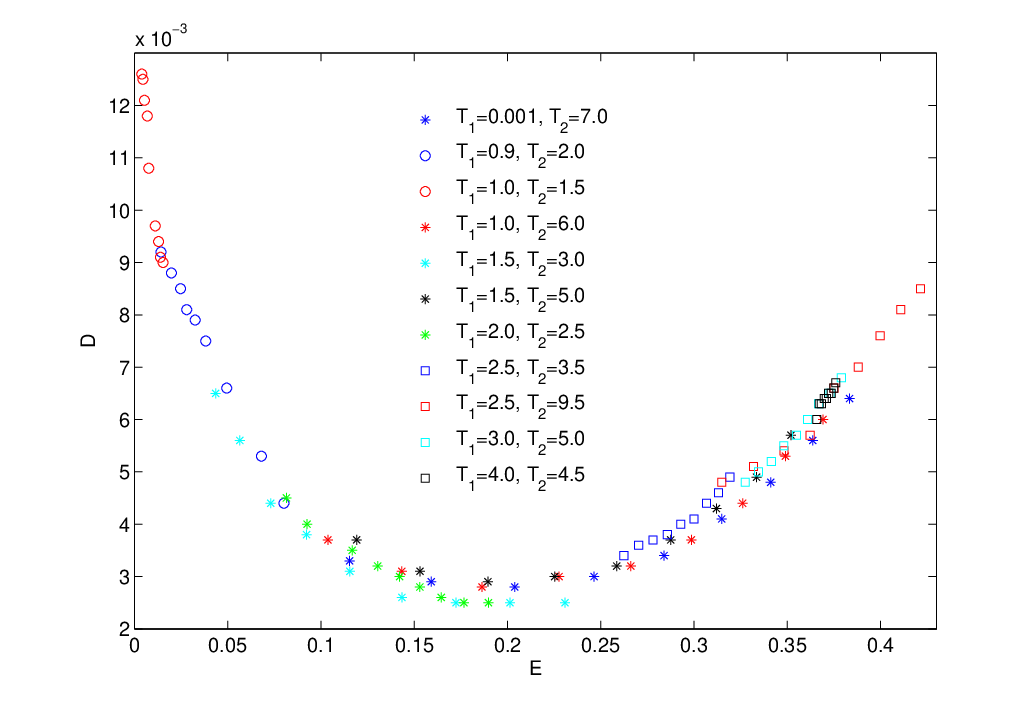
II.2 Thermodynamic observables
Typical quantities considered in [5] are the mean energy densities of the columns, or , where is the column label, and averages run for each on both time and column sites. This may be seen as a particular case of a general frame. By averaging at every time along the direction only, is a discrete time series; analogously for the squared magnetization of the -th column. All typical statistical features of time series, first of all time averages and mean square deviations, may be easily calculated. As usual, well stabilized values out of long runs will be considered equivalent to the asymptotic ideal values for all practical purposes.
An interesting point consists in the systematic comparison between the Ising model with a heat flow (or IMF, for brevity) and the closed Ising model (or CIM), i.e. the two dimensional toroidal lattice whose energy (a constant of motion in this case) will be fixed with suitable criteria. Alternatively, one can compare the IMF and the thermalized Ising model (or TIM) where the flow is zero because the borders are fixed at the same temperature.
More precisely, such comparisons require the following steps: 1 - evaluate the mean energy of a particular column in the IMF; 2 - fix equal border temperatures for the TIM or the total energy of the system for the CIM in such a way that the average energy of any column in these systems is equal to ; 3 - follow the time evolution of the systems (IMF, TIM and CIM) in order to obtain three sequences of decorraleted values for the different observables (e.g. and ); 4 - compute statistical properties of the obtained time series.
These comparisons aim to stress the influence (if any) of the local flow on physical observables with respect to different types of thermalized systems.
Of course, an additional check is the comparison between TIM and CIM, which should converge to the same behaviour for all observables at least when .
II.3 Geometrical observables
In order to give evidence to possible correlations between heat flow and configurational features, we need a different kind of observables. Such observables have already been used to study equilibrium states in spin systems (precisely Ising systems, with or without long range correlations) proving useful in focusing certain peculiarities of configurations around the critical phase [11, 12].
The precise definition of these quantities requires the formalism of configuration and partition spaces, as briefly summarized in the Appendix. However, the main idea is the following: consider the configuration of a column as a discrete periodic array of binary values. A probability measure is easily defined on the array subsets by the normalized number of nodes in each subset. This way, an array (or more precisely the triple constituted by , and the algebra of subsets) becomes a particularly simple example of finite probability space. An array may be partitioned into homogeneous clusters of consecutively aligned spins, and this collection may be seen as an element of the “partition space” built on the probability space . We have established a correspondence between configurations and finite measurable partitions, or, more explicitely
In this case, the natural order of the cluster sequence identifies the partition by the first coordinates of each cluster. Shannon entropy, conditional entropy, Rohlin and Hamming distances between two arbitrary columns are therefore well defined functionals (see Appendix). We shall consider in particular the following observables:
- 1.
the Rohlin distance at a time between partitions and associated to consecutive columns and of the same system, i.e.
this distance is a measure of the non similarity between adjacent columns, with regard to the cluster distributions;
- 2.
the Rohlin distance between decorrelated columns with the same energy (same label ). This is a measure of the non similarity between independent columns. Decorrelated configurations can be obtained considering either two distinct systems evolving independently, or the same system and an evolution time much larger than the decorrelation time. Therefore, the fistances we consider are
respectively.
- 3.
the Hamming distance between two adjacent columns, as in item 1, i.e.:
this is another and very different measure of non similarity, focusing on pointwise differences, independently of the neighborhoods. Moreover, in this case, represents the energy between a column and the next one.
The observables defined above, like the previous thermodynamic quantities, produce discrete time series, admitting statistical analysis (means, deviations, etc.).
III Numerical experiments
As anticipated, numerical experiments tend to stress the influence of the heat flow on significant observables, by comparing IMF and CIM or TIM. Data, in the following, will refer to both time averages and averages over multiple experiments. Time averages extend as usual up to stable results. Actually, averages run over sampled values, ensuring an excellent stabilization, as if, for all practical purposes, the limit had been reached.
III.1 Energy and Magnetization
The first quantity we shall consider is the energy density along the X direction, or , being the label of the array , the configuration of the -th column. For each column the mean in the Y direction is always assumed. Consider a system sampled at times , where the starting occurs after a suitable transient (e.g. 50 to 100 times for ). Moreover, in order to have sufficiently decorrelated configurations, . Several have been tested. The resulting time series depends also on and the border temperatures . Then, for every there is a mean energy density , and a Mean Square Deviation (here stands for fluctuation). Such diagrams are plotted in Fig.2 for and at fixed . Here , and the same in the following, otherwise differently stated. In the same figure, at the prescribed energies , the fluctuations of the closed system (CIM), are plotted. Since they almost coincide for different sizes, only the case is reported, with the error bars. These diagrams show that:
- •
discrepancies between IMF and CIM, defined as
(2) (obviously, this definition may be adapted to various cases and observables), are especially important around the critical energy density , in a range , with very small. Moreover, , i.e. fluctuations are always greater for IMF.
- •
Both the width of and the maximal amplitude of depend on . Indeed, as grows, decreases and discrepancies slowly shrink. The way decreases seems faster in fact than the correlated way the vanishes.
- •
By comparing data relevant to different sizes, we find that, within and sufficiently far from , scales like . As for the very critical point , our numerical data do not allow any accurate prediction about the behaviour of , however, they suggest that decreases slower than , as grows. Interestingly, this can be read as a weak trace of criticality around .
We remark that the neighborhood of a certain column undergoing a heat flow becomes more and more indistinguishable from an equilibrium neighborhood as . Accordingly, it is plausible that the column properties, inasmuch as they are related to the state of its neighborhood, tend to mimic the equilibrium properties in this limit.

In the same spirit, in Fig .3 we can observe, at fixed , the effect of lowering the difference for IMF. The convergence of IMF to CIM is again clear, starting from up to , where is very thin and is smaller and smaller as grows.
Neatly below , or above , the coincidence between IMF and CIM is quite good for all and . A natural question is the reproduction of the same results using a TIM instead of a CIM, i.e. a thermalized system with equal border temperatures, such to give suitable mean energies for comparisons. As a matter of fact, both CIM and TIM give indeed qualitatively equivalent results with respect to IMF; however, at the observed sizes, they do not coincide (see again Fig. 3). One expects, of course, that only for sufficiently high ’s a good agreement will take place.

In general, the observed behaviour confirms a fact already noticed in [5], i.e. enlarging is equivalent to zooming on a system with a lower , so that the thermodynamic limit should give to every column the same features of a system in local equilibrium. Clearly, such a zooming property is not an absolute equivalence, since a finite size TIM cannot reproduce an infinite size IMF. The equivalence refers only to the onset of local equilibrium due to the vanishing of the gradient between left and right side of each column. Moreover, critical properties could disturb the continuity of this process around .
Consider now the squared magnetization , which above the critical energy coincides with the mean square deviation of . For a fixed size (here ), in Fig .4 we plot the mean values of vs. energy: the IMF diagram is neatly above the CIM diagram in the same region previously identified by energy fluctuations, from up to . Hence, in the same domain, also the magnetization fluctuations are larger in the IMF system.

III.2 Metric properties
The energy between a column and the two adjacent ones (X direction) should feel, in principle, the asymmetry between left and right neighbourhoods. Clearly, as remarked in subsection II.3, such a longitudinal energy between close columns coincides with their Hamming distance (see Appendix for definitions), giving this metric concept also a physical interpretation. In Fig. 5, the expected difference between IMF and CIM for this quantity may be easily recognized, once again in the same region previously evidenced by energy density and magnetization.

A quantity directly related to the configurations, more precisely to the cluster distributions, is the Rohlin distance (see Appendix), which may be measured with various attitudes. For generic partitions, is the amount of information necessary to distinguish from , i.e. a measure of their non-similarity. Such a non-similarity, in our case, can regard both spatially or temporally distinct cluster distributions. Since this appears deeply related to the variability of configurations, is a good candidate, in principle, to be an indicator of the influence of a gradient on steady states. First of all, we consider couples of adjacent columns, so that the longitudinal energy is a meaningful alternative abscissa. The mean values and fluctuations of vs. are plotted in Fig. 6 and 7 respectively, confirming the larger variability of IMF system.


It would be also interesting to understand if it is possible to distinguish systems with or without heat flow by looking at a single column. To this end we consider the sequence of uncorrelated configurations at times , calling the corresponding partition for the -th column (see Appendix for details). We calculate the numerical sequence of distances: . Such a sequence follows the “novelty creation” along an orbit for every examined column, whereas the previous sequence followed the evolution of an isochronous gradient of novelty between adjacent columns. In both cases, fluctuations give overall estimates of such dynamic or isochronous variability.
In Fig. 8 we observe the behaviour of time averaged for as a function of the energy of the corresponding columns. For clearness, we have splitted the comparison in two frames, 16-32 and 16-64 respectively. Apart the incidental inversion between IMF and CIM at , at larger , IMF-distances are greater than the corresponding CIM-distances. Once again the larger variability of the system presenting heat flow is evidenced.
We note also that the maximum evolves with : the peak grows logarithmically, as expected, while the peak abscissa slowly decreases.

As to fluctuations, results summarized in Fig. 9 are extremely similar to those in the previous Fig. 7.

Three points have to be stressed:
- •
- •
fluctuations are only slightly wider in the uncorrelated cases;
- •
the region interested by a discrepancy between IMF and CIM is again the same, possibly with a small shift toward low energies for the left bound.
A further remark is that nothing would be different in Fig. 9 using partitions from two independent systems: this confirms the complete decorrelation of configurations along an orbit within .
IV Conclusions and perspectives
All numerical experiments on the Ising cylindrical model converge on the fact that the imposed heat flow reveals in a wider amplitude of fluctuations for local observables. Recalling the robustness of present results with respect to small perturbations of the dynamics, as remarked in (II.1), a natural question arises: how much does this behaviour depend on the IMF peculiarities? In other terms, would an asymmety in the boundary conditions, as the left-right temperature difference in our model, be automatically translated into amplified fluctuations, when imposed on a generic lattice system? If so, being a general consequence of spatial asymmetry in probabilistic processes, this feature would be very weakly related to physics. We would argue, on the contrary, that the observed behaviours of IMF vs. CIM or TIM are non trivially related to real mesoscopic features of a magnetic system.
First of all, a point stressing the physical meaning of our experiments is that the influence of heat flow on observables appears to be deeply related to the peculiar way an Ising rectangular model passes through the critical region. The amplification, as remarked, does not regard indeed the whole of a steady state, but only a relevant neighborhood of the magnetic transition. On the contrary, for small values of and high values of , observables in the regions close to the borders are practically indistinguishable from those in equivalent equilibrium states. This last feature may be understood in terms of typical configurations: near the cold border, there are indeed sparse spots of one or two sites, making the left and right neighborhoods of the observed column practically identical. The same happens near the hot border, provided that the temperature is sufficiently high to establish a uniform disorder, this time because of the irreducible fragmentation into thin clusters. Only in the intermediate region there is a meaningful difference between left and right sides, reflecting the growth and subsequent fragmentation of clusters in the X direction. Columns are slices of such clusters, with a shape dependence on heavily related the properties of the Ising system.
A further indication that an asymmetry in boundary conditions is not sufficient to explain the larger variability of IMF is provided by a simple study of the paradigmatic model of non interacting diffusion, i.e. RW on a lattice. Precisely, by imposing different densities of walkers at the borders, it is possible to show that, even in the presence of a strong density gradient, fluctuations in the system remain unchanged.
Hence, a purely diffusive RW is too poor to reproduce the behaviour we have observed in the Ising model, where evidently interaction plays a fundamental role. In the same way, the very existence of a critical temperature (or energy), which is certainly related to the observed effects, is irreproducible by simple RW. In order to clarify the subject, local interactions should be introduced in the RW model, mimicking the role of the energy dependent diffusivity in IMF. This may be done in several ways, and studies in this direction are in progress, as well as tests on totally different dynamical systems (e.g. asymmetric sandpiles). All this will be fully reported in another paper.
Finally, we remark that the relevance of a finite (i.e. non infinitesimal) thermal gradient, or the consequent vanishing of and in the thermodynamic limit, do not imply that the observed effects are physically meaningless. There are no reasons indeed to consider finite size properties as unphysical. A mesoscopic situation ( finite) with peculiar non-equilibrium features could be equally or even more interesting from a physical point of view.
Acknowledgments
We thank N. Macellari and E. Vivo (Parma) for important discussions in the early phase of the work.
Appendix A Appendix: Configurations, Partitions Spaces and Distances
Let be a graph with nodes or sites assuming values in an alphabet . A configuration on is a whole set . It is an element of , the set of all possible states of the lattice. For instance, if is a discrete array (as in the case of our columns) or a square lattice, and , this description fits Ising-like systems.
A path, is a sequence of “near” sites, and a connected cluster is a set of sites with the same value in which are connected by a path. For general graphs, clusters are connected but not necessarily simply connected sets. Since every site belongs to a single cluster, clusters are disjoint subsets of and . In other terms, the clusters collection is a “finite partition” of , whose subsets constitute its “atoms”. The partition space is the set of all finite partitions of . The correspondence between a configuration and the clusters partition , i.e. , is “many to one”, because configurations generated by permutations in are mapped into the same partition.
For every subset of , let be the normalized number of nodes in . This defines a probability measure in the algebra of subsets of .
For standard operations on partitions in classical textbooks are e.g. [13, 14, 15, 16]. For applications in the spirit of our demands, see also [11, 12, 17, 18]. Here we only recall the definitions of Shannon entropy and Rohlin distance.
Let be a partition: its Shannon entropy is
| (3) |
The Shannon entropy does not depend on the shapes of the atoms, but only on their measures. If is another partition, shapes implicitly influence the conditional entropy of with respect to :
| (4) |
Then, the Rohlin distance between partitions is defined by
| (5) |
This makes a metric space. The Rohlin distance expresses how different two partitions are.
If itself is a metric space (e.g. a numerical set with the usual distance between numbers), one can also consider in the Hamming distance which, for configurations and , is defined by the functional
| (6) |
(possibly normalized by dividing by ). In our case, as noticed in Section III.2, the Hamming distance between adjacent columns is the energy between them.
In general, Hamming and Rohlin distances are not directly comparable. The former is between configurations, and it is sensitive only to actual values of corresponding nodes, not to their distribution or neighborhood, whereas the latter is between partitions, and therefore it is sensitive to the cluster shapes. In principle, and may give very different information. With a binary alphabet, for instance, complementary configurations have maximal Hamming distance (), while the corresponding partitions coincide ().
If a configuration has discrete evolution
one can speak of “configurations orbit”. The corresponding dynamics on is defined by
| (7) |
so that to a configurations orbit there corresponds a partitions orbit . Clearly, the probability measure in is not preserved by , because clusters do not evolve in themselves but are redefined at every step by the pointwise dynamics in . However, we are not interested here in indicators requiring a preserved measure, such as Kolmogorov-Sinai entropy or Lyapunov exponents.
Real valued observables or , in or , give rise to “time series” or . Such time series are typical objects of our investigations.
This formalism applies in principle to every kind of lattices and discrete dynamics. Note however that when is a one dimensional array, as in the case considered here, the Rohlin distance is essentially simpler than in the two-dimensional case, because of the geometrical nature of the atoms contours: points in the former case, possibly cumbersome paths in the latter (see e.g. [11, 12, 18]). For the Hamming distance, on the contrary, the computational complexity would be almost the same.
References
- [1] S. Lepri, R. Livi and A. Politi, Phys. Rep. 377, 1 (2003) 1-80.
- [2] R. Harris and M. Grant, Phys. Rev. B 38 (1988) 9323-9326
- [3] K Saito, S. Takesue and S. Miyashita, Phys. Rev. E 59, (1999) 2783-2794.
- [4] V. Eisler, Z. Racz and F. van Wijland, Phys. Rev. E 67 (2003) 056129-1-9
- [5] M. Casartelli, N. Macellari and A. Vezzani, Eur. Phys. J. B 56 (2007) , 149-156
- [6] A. Dhar and D. Dhar, Phys. Rev. Lett 82, (1999) 480-483.
- [7] G.Y.Vichniac, Physica 10D, (1984) 96-116.
- [8] Y. Pomeau and G.V. Vichniac, J. Phys. A: Math. Gen. 21 (1988) 3297-3299
- [9] T. Toffoli and N. Margolus, Cellular Automata Machines (The MIT Press, Cambridge 1987) 185-205
- [10] L. Kadanoff and J. Swift, Phys. Rev. 165, 1 (1968) 310-322.
- [11] D.Bettati, M.Casartelli, P.Celli and L.Malpeli, J. Phys A: Math. Gen. 31 (1998) 9359-9376.
- [12] M. Casartelli, L. DallAsta, E. Rastelli and S. Regina, J.Phys.A: Math. Gen. 37 (2004) 11731-11740
- [13] P. Billingsley: Ergodic Theory and Information, (J. Wiley, NY 1965).
- [14] V.I.Arnold and A. Avez: Problèmes Ergodiques de la Mécanique Classique (Gauthier-Villars, Paris 1967).
- [15] I.P. Cornfeld, S. V. Fomin and Ya. G. Sinai: Ergodic Theory (Springer-Verlag, 1982).
- [16] N. F. G. Martin and J, W. England: Mathematical Theory of Entropy (Addison-Wesley, Reading MA 1981).
- [17] M.Casartelli, Complex Syst. 4 (1990) 491-507; A. Albrigi and M. Casartelli, Complex Syst. 7 (1993) 171-197
- [18] M.Casartelli and M.Zerbini, J. Phys. A: Math. Gen. 33 (2000) 863-872.