Transition from fractal to non-fractal scalings in growing scale-free networks

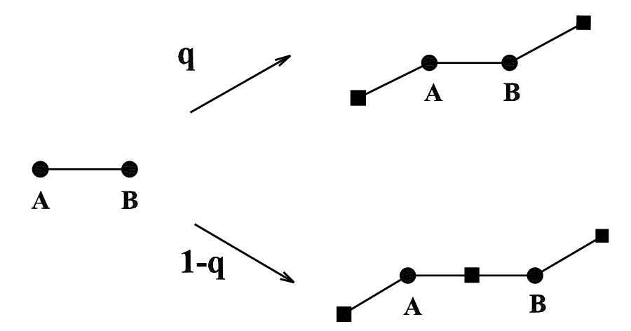
The proposed evolving networks (graphs) have a treelike structure, which are constructed in an iterative way as shown in Fig. 1. Let $T_{t}$ ($t\geq 0$) denote the networks after $t$ iterations. For $t=0$, the networks growth begins from two nodes (vertices) connected by an edge (link or bond). For $t\geq 1$, $T_{t}$ is obtained from $T_{t-1}$. We replace each edge in $T_{t-1}$ either by the path on the top right of Fig. 1 with probability $q$, or by the path on bottom right with complementary probability $1-q$. In other words, $T_{t}$ is generated from $T_{t-1}$ by adding $k_{v}$ leaves to each node $v$, where $k_{v}$ is the degree of node $v$ in $T_{t-1}$. Then, the resulting graph is further modified by expanding each edge with probability $1-q$, which was already present in $T_{t-1}$. Expansion of an edge $(uv)$ means: removal of $(uv)$ and creation of an additional node $w$ with edges $(uw)$ and $(vw)$. (Note that real systems may exhibit such an evolving mechanism. For example, this mechanism has been used to model the network evolution of connected minima on a potential energy landscape [18].) This procedure is iterated $t$ times, with the needed graphs obtained in the limit $t\to\infty$.

As will be shown in next section, when $q=1$, the network is a small world with infinite fractal dimension, its average path length (APL) grows logarithmically with node number. In the particular case of $q=0$, the network is a ‘large’ world with a finite fractal dimension of 2, its APL scales exponentially with network size. Except these two limiting cases of $q=1$ and $q=0$, for other $q$ ($0<q<1$), the networks are growing stochastically. Varying $q$ in the interval (0,1), the networks exhibit a transition from small to large world, and simultaneously show an interesting phenomenon with a transition from non-fractal to fractal behavior.

Note that the current model is similar to the probabilistic model introduced by Song, Havlin, and Makse (SHM Model) in [9]. The construction step with probability $q$ in the current manuscript is analogous to the Mode I growth process in the SHM Model, involving strong hub-hub attraction. And the step with probability $1-q$ is analogous to the Mode II growth process in the SHM Model, involving hub-hub repulsion. The probabilistic mixing of these two types of construction steps leads to the same results in both of the SHM Model and the current model: when $q=1$ (or pure Mode I) is involved, the network has infinite fractal dimension and shows small-world scaling; any $q\leq 1$ (or mixing of Modes I and II) leads to a finite fractal dimension. However, in [9] only part of the properties was addressed. Here we will present an exhaustive analysis of various characteristics, including additional features (such as average path length and betweenness centrality) not calculated in [9].

Now we compute some related quantities such as the number of total nodes and edges in $T_{t}$, called network order and size, respectively. It should be mentioned that as $q$ is a real number, we assume that all variables concerned with $q$ change continuously. Note that a similar assumption was used in Refs. [1, 2, 3, 4], which is valid for large $t$. Let $L_{v}(t)$ be the number of nodes generated at step $t$, $E_{t}$ the total number of edges present at step $t$. Then $L_{v}(0)=2$ and $E_{0}=1$. By construction (see Fig. 1), at each time step, each existing edge is replaced either by three edges with probability $q$ or by four edges with complementary probability $1-q$. Thus, $E_{t}=q\times 3E_{t-1}+(1-q)\times 4E_{t-1}=(4-q)^{t}$ ($t\geq 0$). At the same time, each existing edge yields two or three new nodes with probability $q$ or $1-q$, this leads to $L_{v}(t)=q\times 2E_{t-1}+(1-q)\times 3E_{t-1}=(3-q)(4-q)^{t-1}$ ($t\geq 1$). Then the number of total nodes $N_{t}$ present at step $t$ is

The average node degree after $t$ iterations is $\langle k\rangle_{t}=\frac{2\,E_{t}}{N_{t}}$, which approaches $2$ for large $t$, coinciding with the treelike structure of networks.

When a new node $i$ is added to the networks at a certain step $t_{i}$ ($t_{i}\geq 1$), it has a degree of either 1 or 2. We denote by $k_{i}(t)$ the degree of node $i$ at time $t$. By construction, the degree $k_{i}(t)$ evolves with time as $k_{i}(t)=2\,k_{i}(t-1)$. That is to say, the degree of node $i$ increases by a factor 2 at each time step. Thus, the degree spectrum of the networks is discrete. In network $T_{t}$ all possible degree of nodes is 1, 2, $2^{2}$ $2^{3}$, $\ldots$, $2^{t-1}$, $2^{t}$.

Let $L_{1}(t_{i})$ and $L_{2}(t_{i})$ be the separate number of new nodes with degree 1 and 2 that were born at step $t_{i}$. According to the construction algorithm, we have $L_{1}(t_{i})=q\times 2E_{t_{i}-1}+(1-q)\times 2E_{t_{i}-1}=2\,(4-q)^{t_{i}-1}$ and $L_{2}(t_{i})=(1-q)E_{t_{i}-1}=(1-q)(4-q)^{t_{i}-1}$. Then in network $T_{t}$, the expected number of nodes of degree $k=2^{t-m}$ is $n_{k}=L_{1}(m)+L_{2}(m+1)=(6-5q+q^{2})(4-q)^{m-1}$.

Since the degree spectrum of the networks is not continuous. It follows that the cumulative degree distribution [3] is given by $P_{\rm cum}(k)=\frac{N_{t,k}}{N_{t}}$, where $N_{t,k}=\sum_{k^{\prime}\geq k}n_{k^{\prime}}$ is the number of nodes whose degree is not less than $k$. When $t$ is large enough, we find $P_{\rm cum}(k)\approx k^{-\ln(4-q)/\ln 2}$. So the degree distribution $P(k)$ of the networks follows a power-law form $P(k)\sim k^{-\gamma}$ with the exponent

which is a monotonically decreasing function of $q$. As $q$ increases from 0 to 1, $\gamma$ drops form 2 to $1+\frac{\ln 3}{\ln 2}$ [19].

Shortest paths play an important role both in the transport and communication within a network and in the characterization of the internal structure of the network [5]. Let $d_{ij}$ represent the shortest path length from node $i$ to $j$, then the average path length (APL) $d_{t}$ of $T_{t}$ is defined as the mean of $d_{ij}$ over all couples of nodes in the network, and the maximum value $D_{t}$ of $d_{ij}$ is called the diameter of the network. APL is relevant in many fields regarding real-life networks and has received much attention [20].

For general $q$, it is difficult to derive a closed formula for the APL $d_{t}$ of network $T_{t}$. But for two limiting cases of $q=0$ and $q=1$, both the networks are deterministic ones, which allows one to obtain the analytic solutions for APL. The detailed exact derivation about APL is included in the Appendix section. The obtained results show that the APL for these two particular cases presents qualitatively disparate behaviors: For $q=0$, it is found that

which is approximately equal to $\frac{13\times 2^{t}}{14}$ for large $t$. Since $N_{t}\sim 4^{t}$ for large network, so $d_{t}\sim N_{t}^{1/2}$, indicating that $d_{t}$ grows as a square power of the network order $N_{t}$. This phenomenon is similar to that of the two-dimensional regular lattice [21]. Thus, the network corresponding to $q=0$ is not a small world. For $q=1$, we find

which approximates $\frac{2\,t}{3}$ in the infinite $t$, implying that the APL shows a logarithmic scaling with network order. Therefore, in the specific case of $q=1$, the network exhibits a small-world behavior.

Thus, when we tune $q$ from 0 to 1, the networks undergo a transition from a ‘large’ to small world. We stress that such a transition has already been observed in some previously studied models [22].

As mentioned in preceding subsection, the diameter of a network is defined as the longest shortest path between all pairs of nodes, characterizing the maximum communication delay in the network. Although we do not give a closed formula of APL of $T_{t}$ for general $q$, here we will provide the exact result of the diameter of $T_{t}$ denoted by $D_{t}$.

We first address the network of $q=1$ case, where the shortest distances between existing node pairs are not altered when new nodes enter the systems. For this particular case, $D_{0}=1$. At each time step, the diameter of the network increases by 2. Then the diameter of $T_{t}$ is $D_{t}=2\,t+1$ and thus scales logarithmically with the network order, showing a similar behavior as that of the average path length. Since small diameter is consistent with the concept of ‘small-world’, the additive growth in the diameter with time also (as the APL) suggests that the network for $q=1$ case is a small world.

For $0\leq q<1$, the addition of new nodes affects fundamentally the distances between existing node pairs. By construction algorithm, for any existing couple of nodes connected by a link, after a generation of evolution, the distant $l$ between this pair of nodes may be equal to 1 or 2 with probability $q$ and $1-q$, respectively. Thus the expected value of $l$ is $2-q$. Using this result and considering that the networks are treelike, we can derive the following recursive relation for expected $D_{t}$:

Since $D_{0}=1$, we can resolve Eq. (5) to obtain the average of network diameter as

which grows as a power of time $t$.

To determine the fractal dimension, we distinguish two cases: $0\leq q<1$ and $q=1$. In the case of $0\leq q<1$, we follow the mathematical framework introduced in Ref. [9]. We are concerned about three quantities: network order $N_{t}$, network diameter $D_{t}$, and degree $k_{u}(t)$ of a given node $u$. By construction, we can easily see that in the infinite $t$ limit, these quantities grow obeying the following relations: $N_{t}\simeq(4-q)\,N_{t-1}$, $D_{t}\simeq(2-q)\,D_{t-1}$, $k_{u}(t)=2\,k_{u}(t-1)$. Thus, for large networks, $N_{t}$, $k_{u}(t)$ and $D_{t}$ increase by a factor of $f_{N}=4-q$, $f_{k}=2$, and $f_{D}=2-q$, respectively.

From above obtained microscopic parameters demonstrating the mechanism for network growth, we can derive the scaling exponents: the fractal dimension $d_{B}=\frac{\ln f_{N}}{\ln f_{D}}=\frac{\ln(4-q)}{\ln(2-q)}$ and the degree exponent of boxes $d_{k}=\frac{\ln f_{k}}{\ln f_{D}}=\frac{\ln 2}{\ln(2-q)}$. According to the scaling relation of fractal scale-free networks, the exponent of the degree distribution satisfies $\gamma=1+\frac{d_{B}}{d_{k}}=1+\frac{\ln(4-q)}{\ln 2}$, giving the same $\gamma$ as that obtained in the direct calculation of the degree distribution, see Eq. (2).

For $q=1$, although the number of their nodes increases exponentially, its diameter grows linearly with time. Thus, in this case the network has infinite dimension and does not present a fractal topology.

Betweenness centrality (BC) of a given node is the accumulated fraction of the total number of shortest paths going through the node over all node pairs [24, 23]. More precisely, the betweenness of a node $i$ is

where $\sigma_{jk}$ is the total number of shortest path between node $j$ and $k$, and $\sigma_{jk}(i)$ is the number of shortest path running through node $i$.

We now investigate the BC distribution of nodes. It was claimed in previous studies that for scale-free networks, the BC distribution $P(b)$ of nodes obeys a power law with the exponent $\gamma_{b}=2$, i.e., $P(b)\sim b^{-2}$. It was also suggested that the exponent $\gamma_{b}=2$ is universal for all scale-free networks [25]. Next, we will present that the exponent $\gamma_{b}$ is not universal and constant (at least for fractal trees), but varies significantly as a function of $d_{B}$ (or a function or $q$).

In order to obtain the exponent $\gamma_{b}$ of BC distribution of our networks, we resort to a heuristic argument similar to that applied in [26]. Notice that all of our networks are treelike and fractal (except the case of $q=1$). Considering one network with dimension $d_{B}$, for a small area of the network containing $g$ nodes, its average path length is typically $d(g)=g^{1/d_{B}}$ [27]. All nodes in this small region can reach the rest nodes in the network via $d(g)$ nodes. Thus, the BC of these $d(g)$ nodes is not less than $g$. On the other hand, in the whole network there are $N_{t}/g$ such areas, each of which includes $g$ nodes. Then, the total number of nodes with BC $b$ not less than $g$ in the whole network is

Therefore, the cumulative BC distribution is

which implies $P(b)\sim b^{-\gamma_{b}}$ with

Thus, $\gamma_{b}$ is a increasing function of fractal dimension $d_{B}$, the larger the fractal dimension $d_{B}$, the larger the exponent $\gamma_{b}$. Eq. (10) shows that $\gamma_{b}=2$ holds only for the non-fractal networks with $d_{B}\rightarrow\infty$ [28], where a relatively small number of hub nodes bear large BC. In contrast, in fractal networks, the BC of a lot of ‘small’ nodes can be compared with that of hub nodes.

As shown in Fig. 2, for the $q=0$ case, the network $T_{t+1}$ may be obtained by the juxtaposition of four copies of $T_{t}$, which are labeled as $T_{t}^{\theta}$, $\theta=1,2,3,4$. Then we can write the sum $S_{t+1}$ as

where $\Delta_{t}$ is the sum over all shortest paths whose endpoints are not in the same $F_{t}$ branch. The solution of Eq. (A.3) is

The paths that contribute to $\Delta_{t}$ must all go through at least one of the three edge nodes (i.e., E, F and G in Fig. 2(b)) at which the different $T_{t}$ branches are connected. The analytical expression for $\Delta_{t}$, called the crossing paths, is found below.

Denote $\Delta_{t}^{\alpha,\beta}$ as the sum of all shortest paths with endpoints in $T_{t}^{\alpha}$ and $T_{t}^{\beta}$. If $T_{t}^{\alpha}$ and $T_{t}^{\beta}$ meet at an edge node, $\Delta_{t}^{\alpha,\beta}$ rules out the paths where either endpoint is that shared edge node. If $T_{t}^{\alpha}$ and $T_{t}^{\beta}$ do not meet, $\Delta_{t}^{\alpha,\beta}$ excludes the paths where either endpoint is any edge node. Then the total sum $\Delta_{t}$ is

By symmetry, $\Delta_{n}^{1,2}=\Delta_{t}^{2,3}=\Delta_{n}^{3,4}$ and $\Delta_{t}^{1,3}=\Delta_{t}^{2,4}$, so that

In order to find $\Delta_{t}^{1,2}$, $\Delta_{t}^{1,3}$, and $\Delta_{t}^{1,4}$, we define

Considering the self-similar network structure, we can easily know that at time $t+1$, the quantity $s_{t+1}$ evolves recursively as

Using $s_{1}=7$, we have

On the other hand, by definition given above, we have

and

where $d_{EF}=2^{t}$ and $d_{EG}=2^{t+1}$ have been used. Substituting Eqs. (A.10), (A.11) and (A.12) into Eq. (A.6), we obtain

Inserting Eqs. (A.13) for $\Delta_{x}$ into Eq. (A.4), and using $S_{1}=20$, we have

Inserting Eq. (A.14) into Eq. (A.1), one can obtain the analytical expression for $d_{t}$ in Eq. (3).

Using analogous analysis for the $q=0$ case, we can calculate the APL $d_{t}$ for the case of $q=1$. For simplicity, we use the same symbols used in last subsection to represent the identical notions. For $q=1$ case, the network $T_{t+1}$ may be obtained by joining at the hubs (the most connected nodes) three copies of $T_{t}$ labeled as $T_{t}^{(\psi)}$, $\psi=1,2,3$ [29], see Fig. 3. Then one can write the sum over all shortest paths $S_{t+1}$ as

The solution of Eq. (A.15) is

The paths contributing to $\Delta_{t}$ must all go through at least either of the two hubs ($X$ and $Y$) where the three different $T_{t}$ branches are joined. The crossing paths $\Delta_{t}$ is given by

where $\Delta_{t}^{1,2}$ rules out the paths where either endpoint is node $X$, $\Delta_{t}^{2,3}$ rules out the paths where either endpoint is node $Y$, and $\Delta_{t}^{1,3}$ excludes the paths with an endpoint is either $X$ or $Y$. Again by symmetry, $\Delta_{t}^{1,2}=\Delta_{t}^{2,3}$, so that

In this case, the quantity $s_{t+1}$ evolves as

Since $s_{1}=4$, Eq. (A.19) is solved inductively:

similarly,

and

Substituting the obtained expressions in Eqs. (A.21) and (A.22) into Eq. (A.18), the crossing paths $\Delta_{t}$ is found to be

Inserting Eq. (A.23) into Eq. (A.16) and using the initial condition $S_{1}=10$, we have

Substituting Eq. (A.24) into (A.1), the exact expression for the average path length is obtained as shown in Eq. (4).

References

- (1) R. Albert and A.-L. Barabási, Rev. Mod. Phys. 74, 47 (2002).
- (2) S.N. Dorogovtsev and J.F.F. Mendes, Adv. Phys. 51, 1079 (2002).
- (3) M.E.J. Newman, SIAM Rev. 45, 167 (2003).
- (4) S. Boccaletti, V. Latora, Y. Moreno, M. Chavez and D.-U. Hwanga, Phys. Rep. 424, 175 (2006).
- (5) L. da. F. Costa, F.A. Rodrigues, G. Travieso, and P.R.V. Boas, Adv. Phys. 56, 167 (2007).
- (6) D.J. Watts and H. Strogatz, Nature (London) 393, 440 (1998).
- (7) A.-L. Barabási and R. Albert, Science 286, 509 (1999).
- (8) C. Song, S. Havlin, H. A. Makse, Nature 433, 392 (2005).
- (9) C. Song, S. Havlin, H. A. Makse, Nature Phys. 2, 275 (2006).
- (10) P. Erdös, A. Rényi, Pub. Math. Insti. Hung. Acad. Sci. 5 (1960) 17.
- (11) M. Kitsak, S. Havlin, G. Paul, M. Riccaboni, F. Pammolli, and H. E. Stanley, Phys. Rev. E 75, 056115 (2007).
- (12) M. Hinczewski and A. N. Berker, Phys. Rev. E 73, 066126 (2006).
- (13) Z. Z. Zhang, S. G. Zhou, and T. Zou, Eur. Phys. J. B 56, 259 (2007).
- (14) Z. Z. Zhang, S. G. Zhou, T. Zou, and J. H. Guan, (unpublished).
- (15) H. D. Rozenfeld, S. Havlin, and D. ben-Avraham, New J. Phys. 9, 175 (2007).
- (16) H. D. Rozenfeld and D. ben-Avraham, Phys. Rev. E 75, 061102 (2007).
- (17) M. Hinczewski, Phys. Rev. E 75, 061104 (2007).
- (18) C. P. Massen and J. P. K. Doye, J. Chem. Phys. 127, 114306 (2007).
- (19) S. Jung, S. Kim, and B. Kahng, Phys. Rev. E 65, 056101 (2002).
- (20) A. Fronczak, P. Fronczak, and J. A. Hołyst, Phys. Rev. E 70, 056110 (2004); J. A. Hołyst, J. Sienkiewicz, A. Fronczak, P. Fronczak, and K. Suchecki, Phys. Rev. E 72, 026108 (2005); S. N. Dorogovtsev, J. F. F. Mendes, and J. G. Oliveira, Phys. Rev. E 73, 056122 (2006); Z.Z. Zhang, L.C. Chen, S.G. Zhou, L.J. Fang, J.H. Guan, and T. Zou, Phys. Rev. E 77, 017102 (2008).
- (21) M. E. J. Newman, J. Stat. Phys. 101 819 (2000).
- (22) K. Klemm and V. M. Eguíluz, Phys. Rev. E 65, 057102 (2002); L. Tian, C.-P. Zhu, D.-N. Shi, Z.-M. Gu, and T. Zhou, Phys. Rev. E 74, 046103 (2006); Z. Z. Zhang, S. G. Zhou, Z. Shen, and J. H. Guan, Physica A 385, 765 (2007); Z. Z. Zhang, S. G. Zhou, Z. Y. Wang, and Z. Shen, J. Phys. A 40, 18863 (2007); S. N. Dorogovtsev, P. L. Krapivsky, and J. F. F. Mendes, Europhys. Lett. 81, 30004 (2008).
- (23) M. E. J. Newman, Phys. Rev. E 64, 016132 (2001).
- (24) C. L. Freeman, Sociometry 40, 35 (1977).
- (25) K.-I. Goh, B. Kahng, and D. Kim, Phys. Rev. Lett. 87, 278701 (2001).
- (26) L. A. Braunstein, Z. Wu, Y. Chen, S. V. Buldyrev, T. Kalisky, S. Sreenivasan, R. Cohen, E. López, S. Havlin, and H. E. Stanley, Int. J. Bifurcation Chaos 17, 2215 (2007).
- (27) Fractals in Science, edited by A. Bunde and S. Havlin (Springer, Berlin, 1996).
- (28) C.-M. Ghima, E. Oh, K.-I. Goh, B. Kahng, and D. Kim, Eur. Phys. J. B 38, 193 (2004); Z. Z. Zhang, S. G. Zhou, L. C. Chen, J. H. Guan, L. J. Fang, and Y. C. Zhang, Eur. Phys. J. B 59, 99 (2007).
- (29) E. Bollt, D. ben-Avraham, New J. Phys. 7, 26 (2005); F. Comellas, H. D. Rozenfeld, D. ben-Avraham, Phys. Rev. E 72, 046142 (2005).