N. Ryzhanova1,2, A. Vedyayev1,2, A. Pertsova2, B. Dieny1Affiliation: 1SPINTEC, URA 2512 CEA/CNRS, 38054 Grenoble Cedex 9, France
2Physics Department, M.V. Lomonosov Moscow State
University, Leninskie Gory, 1199991 Moscow, Russia
August 24, 2026
Abstract
Quasi-two-dimensional transport is investigated in a system consisting of
one ferromagnetic layer placed between two insulating layers. Using
the mechanism of skew-scattering to describe the Extraordinary Hall
Effect (EHE) and calculating the conductivity tensor, we
compare the quasi-two-dimensional Hall resistance with the resistance
of a massive sample. In this study a new mechanism of
EHE (geometric mechanism of EHE) due to non-ideal interfaces
and volume defects is also proposed.
pacs
75.47.-m, 75.70.-i, 73.50.-b
I Introduction
Recently there has been an increased focus on the
fabrication of new spintronic devices based on the tunnel
magnetoresistance effect (TMR)[1] and the
recently discovered spin torque effect (ST)[2]
in multilayered structures consisting of several ferromagnetic
nanolayers separated by thin insulating barriers. The geometric
parameters of such structures also give us the possibility to
investigate some of their quasi-two-dimensional transport
properties and particularly to compare the relationship between
diagonal and off-diagonal (responsible for EHE) conductivities
in massive and above mentioned samples. This study is of great
interest to the field of spintronics since quasi-two-dimensional
EHE may provide an additional mechanism for recording and storing
information in logic devices. Focusing on this aspect of EHE
we study both diagonal and off-diagonal (Hall) conductivities
in a system consisting of one ferromagnetic layer of
thickness placed between two insulating layers and magnetized
in the direction perpendicular to the interfaces (direction).
The remainder of the paper is organized as follows. In Section II
EHE is attributed to the mechanism of skew-scattering[3]
on the bulk and interface impurities. We report our results for
the conductivity tensor including size effect terms calculated
within the framework of the Kubo formalism and compare the
quasi-two-dimensional Hall resistance with
that of a massive sample . Section III
discusses the nonideality of the interfaces and the existence
of volume defects that influence the form of current lines.
We propose a new mechanism of EHE (we will refer to it
as the geometric mechanism of EHE) due to these
defects using the diffusion equation[4] and
taking into account that the diffusion coefficient has
off-diagonal component proportional to the spin-orbit
interaction. We summarize our results and offer some conclusions
in Section IV.
II Skew-scattering mechanism of EHE in a three-layered structure
We will consider the geometry of current parallel to the
direction resulting in the appearance of the component
of the Hall field. In this case:
(1)
where are diagonal and
off-diagonal conductivities, is the Hall field.
For the calculation of we will use
the Kubo formula with vertex corrections responsible for
the transverse component of the current:
(2)
where is the velocity vector along the interface,
, are advanced and retarded
Green’s functions in mixed coordinate-momentum representation. To calculate
the component of the conductivity tensor we will use the perturbation
theory and will take into account only the corrections in linear order of
the spin-orbit interaction:
(3)
(4)
where and
are the scattering matrix and the spin-orbit interaction, correspondently, dependant
on the type of atom in position ; is the unit vector along
the magnetization, is the spin-orbit parameter and is
the lattice constant. It follows from Eq. (4) that .
For the matrix in one-site approximation we can write down:
(5)
(6)
where is the one-site energy. For the binary system
and take values and , respectively; .
is the coherent potential and can be found from the system of self-consistent equations.
The first equation of the system is valid for scattering on both bulk and interface impurities:
(7)
while the second one is written in the form corresponding to the interface scattring since we are interested in calculation of the interface coherent potential:
(8)
For the calculation of , we will use Eq.
(2) with Green’s functions diagonal on and renormalized
on the coherent potential. For off-diagonal component averaging on the
impurities distribution gives:
(9)
where is the impurity position. We keep in Eq.
(9) only the main term with .
For the binary structure and purely random distribution of , summing
over will give .
It is convenient to divide into average and scattering parts:
Usually it is convenient to choose .
In this case , , .
Next we assume that scattering parameters for
bulk impurities such as scattering potential
and concentration are small enough to keep only
the main terms for all values. In this case the
imaginary part of is of order
so for we will use:
(17)
For the interface values the full self-consistent scheme
is necessary. For both bulk and interface we suppose that
the real part of the coherent potential just represents
the renormalization of electron spectrum so can
be considered as purely imaginary.
The zero order Green’s function found from Schrödinger
equation in representation is (we
will further use the units with energy dimension ):
(18)
(19)
(20)
(21)
(22)
where and are the coordinates of the left and
right interfaces, is the layer thickness;
, are the Fermi momentum and
the mean free path for spin "up", respectively,
(for spin "down" we will use index 2);
is the height of the potential barrier.
The poles of the Green’s function in Eq. (18) define
the quantized energy spectrum of the thin ferromagnetic layer.
II.1 Calculation of the bulk quasi-two-dimensional diagonal conductivity
For in Eq. (2) we will take
into account scattering on the interface responsible for size
effect as well as on the bulk of the sample by using the Dyson
equation with renormalized Green’s function:
(23)
Integrating over from to for and from
to for gives the conductivity in the units :
(24)
(25)
(26)
where is the elementary conductivity of one channel.
For large enough layer thickness we can average Eq. (24) over
oscillations so that the averaged conductivity is:
(27)
The first term in Eq. (27) is the conductivity of the massive
sample and the second one is due to the quasi-classical size effect.
The full conductivity representing the sum of two spin channels is
shown on Fig. (1) as a function of the layer thickness.
Figure 1: Averaged diagonal conductivity as a function
of (thickness):
for , , , , (see Eq. (27))
II.2 Calculation of the off-diagonal conductivity due to the spin-orbit interface scattering
Now we will calculate using
Eq. (9) with Green’s function defined by Eq. (23)
and . After integration over the conductivity is:
(28)
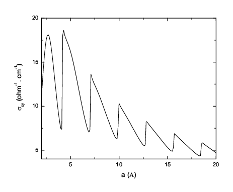
This conductivity oscillates with the thickness and the distance
from the interface . Its behavior becomes more clear after
averaging over oscillations:
(29)
The same is done for spin "down". The sum of these two terms is shown
on Fig. (2).
Figure 2: Off-diagonal conductivity as a function
of (thickness): for ,
, , ,
, (see Eq. (28))
It is clear that decreases with since the functions
have maximum values at . Averaging over these functions gives the factor so for infinite this term tends to zero.
We also calculate the bulk conductivity
(see Fig. (3)) using Eq. (9) with additional integration
over and bulk scattering parameters with the bulk coherent potential in Bohrn approximation .
In the absence of the interfacial scattering this approach gives us:
(30)
(31)
or after averaging over oscillations:
(32)
Figure 3: Bulk off-diagonal conductivity as a function
of (thickness): for ,
, , , ,
, (see Eq. (30))
This conductivity has an oscillating behavior for the thin layer but tends to the constant
value when which coincides with its value for the massive sample.
If we take into account the interfacial scattering the expression for becomes
too complicated so we don’t show it here. But the thickness dependences of
and calculated using the full formula with
renormalized Green’s function are presented at Fig. (4) and Fig. (5),
correspondently. The bulk parameters are: , ,
.
Figure 4: Bulk off-diagonal conductivity with interfacial scattering as a function
of (thickness): for ,
, , Figure 5: Hall angle as a function
of (thickness); bulk parameters: , ,
; interface parameters: ,
,
III Geometric mechanism of EHE
Let us consider an electric current through a thin ferromagnetic layer
of thickness located between two thin insulating barriers and magnetized
in direction perpendicular to the interfaces. The interfaces are not ideal
and besides the impurities have topological defects which will be modeled as
cylinders of radius so that the current lines in the vicinity of these defects
follow their shape.
Diffusion equations for charge and spin currents in the absence of precession are:
(33)
(34)
For the stable state solution . For currents we have the system of equations:
(35)
(36)
(37)
(38)
Here we take into account that , are
the electric field and spin accumulation correspondently,
are the components of diffusion coefficient tensors. Off-diagonal components
and of these tensors are proportional to the spin-orbit
interaction and they are antisymmetrical in the transposition. For
a metal with the cubic symmetry , .
Then we insert Eq. (35)-(38) into Eq. (33) and Eq. (34)
and after some manipulations we obtain two equations:
(39)
(40)
And for :
(41)
For the cylindrical defect shape it is convenient to search for solution in
polar coordinates so we can rewrite Eq. (41):
(42)
where is the angle between axe and the radius-vector
with the coordinates .
Taking into account Eq. (39) we can rewrite Eq. (35) and Eq. (36):
(51)
(52)
Now it is convenient to use the polar coordinate system and to write down
and projections of the currents. Then we can use the boundary
conditions to find unknown coefficients. These projection are:
(53)
(usual term)
(54)
(additional diffusion term)
Now we will make some transformations:
(55)
(56)
Using the expressions for derivatives of , over , ,
which is not too difficult to obtain, we write down the charge and spin
currents in polar coordinates:
(57)
(58)
(59)
(60)
To find the unknown coefficients in Eq. (47) and Eq. (50)
we will use the boundary conditions on the surface of the cylinder
representing that projection of currents are equal to zero:
(61)
It gives us the system
(62)
with solution
(63)
Spin current projection is also zero, and we can write down:
(64)
Then we use some properties of Bessel functions[5]:
Now we can define the additional Hall field due to this cylindrical interface defect
considering that Hall electrodes are the surfaces with
coordinates and . This field is proportional to ,
, . After integrating
over from to for the left surface and from to
for the right one we will have:
(73)
The second term due to is:
(74)
At last, we have to multiply Eq. (73) and Eq . (74) by
the concentrations of defects and electron charge.
IV Conclusion
It was shown that due to the additional scattering of electrons on the
defects of the metal-insulator interfaces the total conductance decreases.
From Eq. (27) it follows that for small values of the ratio
the bulk conductivity is completely suppressed and effective
conductivity is proportional to the effective scattering length on the
interfaces instead of the bulk mean free path. Hall conductivity, if we don’t
take into account the additional scew-scattering on the interface,
decreases with decreasing the thickness of the ferromagnetic metallic layer.
However the contribution to the Hall conductivity due to the additional
scew-scattering on the interface increases. So the important characteristic
of the considered device, Hall angle , is larger for the thin ferromagnetic layer
compared to the bulk layer. Besides that, the influence of insulator columns
penetrating into the metallic layer may further increase the value
of the Hall effect.
Acknowledgements.
N. Ryzhanova and A. Vedyayev are grateful to SPINTEC for hospitality. This work
was partially supported by the Russian Foundation for Basic Research.
References
[1] J. S. Moodera, L. R. Kinder, T. M. Wong and R. Meservey, Phys. Rev. Lett. 74, 3273 (1995).
[2] J. C. Slonczewski, J. Magn. Magn. Mat. L1, 159 (1996).
[3] R. Karplus and J. M. Luttinger, Phys. Rev. 95, 1154 (1954).
[4] S. Zhang, P. M. Levy and A. Fert, Phys. Rev. Lett. 88, 236601 (2002).
[5] A. N. Tikhonov and A. A. Samarskii, Equations of Mathematical Physics (PERGAMON PRESS, Oxford-London, New-York, Paris, 1963), p. 656.