Void Traversal for Guaranteed Delivery in Geometric Routing
Abstract
Geometric routing algorithms like GFG (GPSR) are lightweight, scalable algorithms that can be used to route in resource-constrained ad hoc wireless networks. However, such algorithms run on planar graphs only. To efficiently construct a planar graph, they require a unit-disk graph. To make the topology unit-disk, the maximum link length in the network has to be selected conservatively. In practical setting this leads to the designs where the node density is rather high. Moreover, the network diameter of a planar subgraph is greater than the original graph, which leads to longer routes. To remedy this problem, we propose a void traversal algorithm that works on arbitrary geometric graphs. We describe how to use this algorithm for geometric routing with guaranteed delivery and compare its performance with GFG.
I Introduction
Geometric routing is a promising approach for message transmission in ad hoc wireless networks. Unlike traditional ad hoc routing, geometric routing algorithms have no control messages or routing tables, the nodes maintain no information about data messages between transmissions and each data message is of constant size. Hence, geometric routing is quite scalable. Geometric routing is particularly appropriate for wireless sensor networks. Networked sensors usually have limited resources for routing information, yet many applications for sensor networks require ad hoc configurations of large scale.
In geometric routing, each node knows it own geographic coordinates. Each node is also aware of the coordinates of other nodes and links in a part of the network around it. The coordinates are either obtained from GPS receivers or a localization algorithm [1]. The source node of a data message has the coordinates of the target but the source does not know the complete route to it. The source selects one of its neighbors and sends the message to it. After getting the message the receiver forwards the message further. The objective of the algorithm is to deliver the message to the target.
The simplest version of a geometric routing algorithm is greedy routing. In greedy routing the source, as well as each intermediate node, examines its neighboring nodes and forwards the message to the one that is the closest to the target. Unfortunately, the greedy routing algorithm fails if the message recipient is local minimum: all its neighbors are further away from the target than the node itself. In compass routing [2], the next hop is selected such that the angle between the direction to the next hop node and to the destination is minimal. However, compass routing livelocks even on planar graphs.
GFG [3] (also known as GPSR [4]) is the first algorithm that guarantees delivery of the message. The algorithm is designed for planar graphs. It uses greedy routing. To get out of a local minimum GFG sequentially traverses the faces of the planar graph that intersect the line between the source and target. GFG assumes that the original communications graph is a unit-disk graph. For this graph, the authors construct its Gabriel subgraph. This subgraph preserves the connectivity of the original graph and it can be constructed locally by each node. Datta et al [5] propose further improvements to GFG. Kuhn et al [6] present a similar algorithm with asymptotically optimal worst-case performance.
Our contribution. The guaranteed delivery geometric
routing algorithms, of which we are aware, have the following
shortcoming. Their local minimum avoidance part runs over a planar
graph. The efficient construction of a planar graph requires that the
original graph is unit-disk. As recent work [7] demonstrates
this assumption is not realistic for connection topologies formed by
common networked sensors such as Berkeley motes
[8]. Motes’ radio propagation patters prove to be
quite intricate.
In this paper we demonstrate how to carry out geometric routing with guaranteed delivery on arbitrary non-planar graphs. The foundation of our approach is a void traversal algorithm. We describe algorithms VOID-1 and VOID-2 that incorporate void traversal for routing across the whole network. We also present GVG — an algorithm that uses greedy routing and void traversal to get out of local minima. The void traversal is based on each node storing the network topology of its neighborhood. The neighborhood size needs to meet a condition we call intersection semi-closure. Most practical geometric graphs meet this condition such that the storage requirements for each node are independent of the size of the network and rather small.
We compared the performance of VOID-2 with FACE-2 which is the foundation of GFG. We used randomly generated graphs as a base for comparison. A large number of graphs did not have unit-disk subgraphs. Hence FACE-2 cannot be run. On graphs where FACE-2 and VOID-2 are run, depending on the graph generation parameters, the paths selected by VOID-2 were 35-75% shorter. The memory storage requirements for VOID-2 were independent of the network size and only modestly increased compared to those of FACE-2.
Paper organization. This paper is organized as
follows. We give definitions and describe our notation in Section
II. We present our void traversal algorithm in Section
III. In Section IV we describe how this
algorithm can be used for geometric routing. In Section V
we describe the results of the performance comparison of the void
traversal versus face traversal algorithms. Section
VI concludes the paper.
II Preliminaries
Notation. We model a sensor network as a geometric graph. A geometric graph is a set of nodes (vertices) on a Euclidean plane connected by edges . The number of nodes is . Such graph is planar if its edges intersect only at vertices. Void is a region on a plane such that any two points of this region can be connected by a curve that does not intersect any of the edges of the graph. A boundary of a void contains the segments of the edges adjacent to the void. In every finite graph there is one unbounded external void. A void in a planar graph is face. Observe that the boundary of a face forms a simple cycle. Moreover, each edge of a planar graph borders at most two faces. An edge of a non-planar graph may contain the segments of the borders of arbitrarily many faces.
Neighborhood of a node is a subgraph of . A neighborhood relation over graph associates each vertex of with a subgraph of . Denote an edge between nodes and . Denote a path from to . Denote also the Euclidean distance between and .
Intersection semi-closure.
Definition 1
A neighborhood relation over a geometric graph is -incident edge intersection semi-closed (or just -intersection semi-closed) if, for every two intersecting edges and , either:
- •
there exist , , either one no more than hops and , and belong to ; or
- •
there exist , , either one no more than hops and , , and belong to .
The attractive feature of the intersection semi-closed neighborhood relation is that for any edge , the information about every edge that intersects as well as how to reach such edge is contained in the union of and . Observe that for a particular graph, depending on the value of , such a relation may not exist. However, for any graph there always exists a -incident edge semi-closed relation.
To illustrate Definition 1, we apply it to unit-disk graphs. Unit-disk graph is a geometric graph where two nodes and are connected by an edge if an only if .

Lemma 1
A neighborhood relation over a unit-disk graph is 2-intersection semi-closed if for every node and every edge such that and it follows that .
Proof:By definition is 2-intersection semi-closed if for every edge and every edge intersecting , and the route to and are either in or . These routes are no longer than 2 hops.
Let and be according to the conditions of the lemma. Since is unit-disk, if and then and . According to the conditions of the theorem, both of these edges as well as itself belong to . If this is the case, then both the route to the endpoints and the edge itself belong to . Moreover, these routes are at most 1-hop long. Hence, the definition of intersection semi-closure is satisfied. Similar argument applies to .
Suppose that and . Refer to Figure 1 for illustration. Since intersects , could not be further away from than . Hence, and . Since is a unit-disk, and . By the conditions of the lemma and . Suppose that is closer to than to . Then, the the distance between and is at most . By the conditions of the lemma . Which means that contains the edge and, since also contains , contains the routes to both and . Moreover, the is just 2-hops long: . The argument for is similar. The lemma follows.
Geometric routing. Consider a connected geometric graph , a neighborhood
relation over it and a pair of nodes .
Source has a message to transmit to target . The source knows
the coordinates of the target. The message may be transmitted via
intermediate nodes. Each node may potentially add data to the
transmitted message. In the sequel we ignore the payload of the
message and assume that it contains only the routing information.
A routing algorithm specifies a procedure for intermediate node selection. A geometric routing algorithm with guaranteed delivery ensures the eventual message delivery under the following two constraints: each node receiving the message, selects the next node only on the basis of and the contents of the message received; the message size is independent of network size. Observe that the nodes are not allowed to keep any information about the transmitted message after it has been forwarded.
III Void Traversal Algorithm

Overview. The algorithm traverses an internal void clockwise following the segments of the edges that comprise the border of the void. The external void is traversed counter-clockwise. Refer to Figure 2 for the illustration. Given an edge, for example , that contains the segment of the void’s border, the algorithm has to select the next edge. For this the algorithm needs to determine the ends of the segment of that borders the void. One of the ends — is the intersection of the previous edge and . The other end — is the point of the intersection of and another edge such that is closest to in the direction of the traversal of the void.
Recall that in the intersection semi-closed neighborhood relation, the union of the neighborhoods of and contains every edge intersecting as well as a route to this edge. Hence, to accomplish its objective the algorithm has to examine the neighborhoods of and .
Details. The algorithm uses two types of messages: edge_change, and
edge_selection. edge_change contains: previous edge,
current edge and the direction of the traversal of the current
edge. edge_selection message contains: previous edge, and
suggested next edge.
When a node receives edge_change message from node , it determines the intersection point between the previous edge and the current edge . Notice that the intersection point may be itself. Then examines to find the edge whose intersection point is the closest to in the direction of traversal. This edge is the suggested next edge. Note that the graph is intersection semi-closed and may not contain some of some edges that intersect . For example: .
Hence, selects as the suggested next edge. Edge intersects at point . If does not find any edge that intersects , it keeps the suggested next edge field empty. Node sends edge_selection to the other node incident to the current edge.
When node receives edge_selection from , compares the suggested next edge that receives from with the edges in . If finds an edge intersecting whose intersection point is closer to than , then makes the suggested next edge. Otherwise, the suggested next edge remains the same. If neither nor find the suggested next edge in this manner, considers the edges incident to itself. Node selects the edge nearest to counter-clockwise.
Node forms an edge_change message. This message contains as the previous edge and as the current edge. From the information contained in edge_selection that receives from , is able to determine the direction of the traversal of . The traversal direction is included in edge_change.
After composing edge_change, sends this message to either or . Since the graph is intersection semi-closed, may not contain the route to either nodes. In this case returns the message to and forwards it to the appropriate node.
The above discussion is summarized in the following theorem.
Theorem 1
The Void Traversal Algorithm correctly traverses an arbitrary void in a geometric graph with intersection semi-closed neighborhood relation.
IV Using Void Traversal
to Guarantee Delivery
VOID-1 and VOID-2. The geometric routing algorithms we discuss are VOID-1 and VOID-2. They are rather straightforward extensions of algorithms FACE-1 and FACE-2 respectively. The latter two are planar graph geometric routing algorithms presented by Bose et al [3]. FACE-1 has a better worst-case performance. However FACE-2 is more efficient in practice. Hence, we describe VOID-2 in detail and mention briefly how VOID-1 is designed. Our algorithms are based on the following observation.
Proposition 1
Let and be two arbitrary points on the edges or vertices of a geometric graph. Let be the void such that lies on its border and the line segment intersects . If there is a point where intersects the border of then .
| Algorithm: VOID-2 | ||
| repeat | ||
| /* let be the void with on | ||
| its boundary that intersects */ | ||
| traverse until reaching | ||
| an edge containing point | ||
| intersecting | ||
| until /* target reached */ |
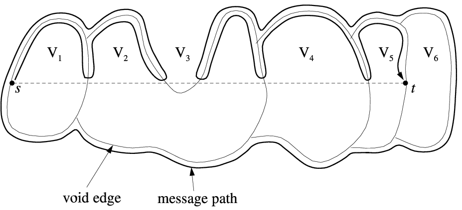
Both VOID-1 and VOID-2 sequentially traverse the voids that intersect the line . Refer to Figure 3 for illustration. While traversing a void, VOID-1 and VOID-2 look for an intersection point with line . Observe that there may be multiple such points. For example, void in Figure 3 has four such points. VOID-1 and VOID-2 differ in their actions when an intersection point is encountered. VOID-1 traverses the whole void, selects the intersection point that is closest to , moves the message to this point and switches to the traversal of the next void. For example, VOID-1 would traverse completely and switch to . VOID-2, on the other hand, switches to the next void as soon as the first intersection point is found. The pseudocode for VOID-2 is given in Figure 4 and an example route that VOID-2 selects is shown in Figure 3.
On the basis of Theorem 1 and the discussion above we state the following.
Theorem 2
Given an arbitrary geometric graph, an intersection semi-closed neighborhood relation and an arbitrary pair of nodes in this graph, both VOID-1 and VOID-2 eventually deliver a message from the first node to the second.
GVG. As in GFG, void traversal is only needed for a
message to leave a local minimum. Otherwise greedy routing can be
used. Care must be taken to avoid a livelock when message returns to
the same local minimum. The complete algorithm –
greedy-void-greedy (GVG) works as follows. The message is at
first forwarded according to greedy routing. When a node discovers
that it is a local minimum, it notes the distance to target and the
routing switches to VOID-1 or VOID-2. The routing switches back to
greedy if the distance to target is less than that of the local
minimum. The process repeats if necessary. Observe that, according
to Theorem 2, the delivery of a message by either VOID-1
or VOID-2 is guaranteed. Hence, either GVG eventually switches to
greedy routing or delivers the message to the target. Hence the
following theorem.
Theorem 3
Given an arbitrary geometric graph, an intersection semi-closed neighborhood relation and an arbitrary pair of nodes in this graph, GVG eventually delivers a message from the first node to the second one in that pair.
V Performance Evaluation
Note that the greedy phase of GFG and GVG is the same. Hence we only compare the performance of local minimum avoidance parts: void and face traversal. We use FACE-2 and VOID-2 for comparison as they are more efficient in practice then FACE-1 and VOID-1.
As a primary metric we compare the length, in the number of hops, of the routes selected by face and void traversal algorithms. Note that a void traversal algorithm makes routing decisions on the basis of larger neighborhood information. Therefore, we compared the individual node memory requirements for face and void traversal algorithms as well.
Graph Generation. We used randomly generated sets of
graphs with 50, 100 and 200 nodes in a fixed area of 2 by 2 units. The
nodes were uniformly distributed over the area. We used a rather
simple model for fading effect of radio reception. For each set of
graphs we selected the connectivity unit to be , and
respectively. We also selected a fading factor to be either
, and . The connectivity between nodes was determined as
follows. We deterministically added an edge for every pair of nodes
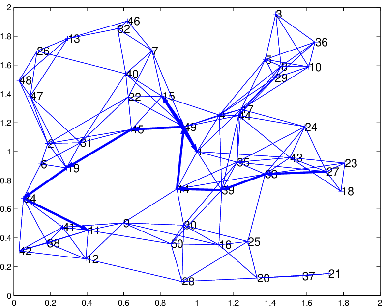
that were no more than away from each other. See Figure
5. If the distance between two nodes was between
and , the edge between them is added
probabilistically. The probability linearly decreased from to
. Notice that when the fading factor is equal to one, the
random graphs that we generated were unit-disk.

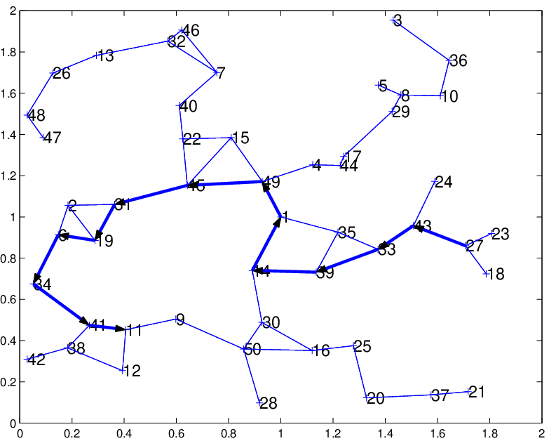
In order to compare FACE-2 and VOID-2 we needed to compute unit-disk subgraphs of the the generated graphs. However, frequently the subgraphs were disconnected: out of 350 of randomly generated 50-node graphs with either or , only a single graph had a connected unit-disk subgraph. These subgraphs had to be discarded as unsuitable for FACE-2. To make the performance comparison, we adopted a different graph selection strategy. We generated random, connected unit-disk graphs and added extra links according to the connectivity rules above. Notice that this strategy favors FACE-2 as it discounts the graphs that are not usable by FACE-2.
We generated 5 graphs for each number of nodes and fading factor. This yielded the total of 45 graphs and their planar subgraphs.
Route Length Comparison. We implemented the FACE-2 and
VOID-2 algorithms in Java and Matlab. We generated 10 random pairs of
nodes for each set of graphs and used VOID-2 and FACE-2 to compute the
routes between the nodes in each pair. VOID-2 used the original graph
and FACE-2 — its unit-disk based planar subgraph. The
example routes are shown in Figure 6.
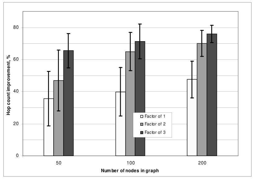
We used paired comparison to estimate the improvement from FACE-2 to VOID-2 in the length of the selected routes as follows. For each pair of source and destination nodes we calculated the difference in the hop-count between routes and normalized it to the hop count of the route selected by FACE-2. That is the comparison is based on the formula: . Figure 7 summarizes the results. Observe that even on unit-disk graphs (), VOID-2 generates routes that are 35-45% shorter than the routes selected by FACE-2. The relative performance of VOID-2 further improves as the fading factor and density of the graphs increases.
Memory Usage Comparison. In both VOID-2 and FACE-2, each
node stores the information about its neighborhood nodes .
The size of the neighborhood differs in the two algorithms. In
evaluating the memory usage, we estimated the average size of the
neighborhood. For the FACE-2, the average size of the neighborhood is
the average degree of the planar subgraph. In our experiments, the
average size of neighborhood in VOID-2, was found to be
where is the fading factor.
VI Conclusion
The elegance and efficiency of geometric routing algorithms is remarkable. Recent advent of large-scale wireless sensor networks increased the relevance of such algorithms. However, the algorithms’ demand for unit-disk based graph planarity hampered the attractiveness of geometric routing. With this paper, we lift this restriction and help the adoption of geometric routing algorithms as the routing solution of choice in sensor networks.
Acknowledgments
We would like to thank Ivan Stojmenovic of the University of Ottawa and M. Kazim Khan of Kent State University for their helpful comments.
References
- [1] N. Bulusu, J. Heidemann, D. Estrin, and T. Tran, “Self-configuring localization systems: Design and experimental evaluation,” ACM Transactions on Embedded Computing Systems, vol. 3, no. 1, pp. 24–60, Feb. 2004.
- [2] E. Kranakis, H. Singh, and J. Urrutia, “Compass routing on geometric networks,” in Proceedings of the 11th Canadian Conference on Computational Geometry (CCCG-99), Vancouver, BC, Canada, Aug. 1999, pp. 51–54.
- [3] Bose, Morin, Stojmenovic, and Urrutia, “Routing with guaranteed delivery in ad hoc wireless networks,” in Wireless Networks: The Journal of Mobile Communication, Computation and Information, Kluwer, 2001, vol. 7.
- [4] B. Karp and H. T. Kung, “GPSR: Greedy perimeter stateless routing for wireless networks,” in Proceedings of the 6th Annual International Conference on Mobile Computing and Networking (MOBICOM-00). N. Y.: ACM Press, Aug. 6–11 2000, pp. 243–254.
- [5] S. Datta, I. Stojmenovic, and J. Wu, “Internal node and shortcut based routing with guaranteed delivery in wireless networks,” Cluster Computing, vol. 5, no. 2, pp. 169–178, Apr. 2002.
- [6] F. Kuhn, R. Wattenhofer, and A. Zollinger, “Asymptotically optimal geometric mobile ad-hoc routing,” in Proceedings of the 6th International Workshop on Discrete Algorithms and Methods for Mobile Computing & Communications (DialM-02). New York: ACM Press, Sept. 28 2002, pp. 24–33.
- [7] D. Ganesan, B. Krishnamachari, A. Woo, D. Culler, D. Estrin, and S. Wicker, “Complex behavior at scale: An experimental study of low-power wireless sensor networks,” UCLA, Technical Report CSD-TR 02-0013, 2002.
- [8] J. Hill and D. Culler, “Mica: A wireless platform for deeply embedded networks,” IEEE Micro, vol. 22, no. 6, pp. 12–24, Nov./Dec. 2002. [Online]. Available: http://dlib.computer.org/mi/books/mi2002/pdf/m6012.pdf; http://www.computer.org/micro/mi2002/m6012abs.htm