Friedel phase discontinuity and bound states in the continuum in quantum dot systems

In a early work, von Neumann and Wigner [1] showed that for certain local potentials, the Schrödinger equation has exact solutions with energy eigenvalues above the continuum threshold. These potentials can be constructed in one dimension by a method suggested in the same article. Much later, several theoretical and experimental works show the existence of these “bound states in the continuum” (BICs) in different contexts. In Ref. [2] it is shown that these states can occur in a system of coupled square well potentials for appropriate values of the well depths and coupling strengths. Stillinger and Herrick corrected and extended von Neumann work to consider systems in two dimensions [3], constructing some potentials leading to BICs. Friedrich and Wintgen demonstrated that BICs occur in natural way, not only for specific potentials, when two resonances associated with different channels interfere [4]. In transport through mesoscopic and nanoscopic systems, there are theoretical works showing the formation of these states in a four-terminal junction [5], in a ballistic channel with intersections [6], and more recently, bound states in the continuum have been theoretically discussed for systems of quantum dots [7, 8, 9, 10]. The existence of BICs in open quantum billiards with variable shape is discussed in Ref. [11], and in a single-level Fano-Anderson model with a colored interaction with the continuum in Ref. [12]. An experimental evidence of BICs was reported by Capasso et al. [13] in semiconductor heterostructures grown by molecular beam epitaxy.

The density of states (DOS) is of great relevance to understand transport phenomena. The DOS is related to the scattering matrix $S$ via the Friedel sum rule (FSR), which can be stated as

where the Friedel phase $\theta_{F}$ is defined as

where the phase shifts $\xi_{l}$ are obtained from the eigenvalues of the scattering matrix $S$, $\lambda_{l}=e^{2i\xi_{l}}$ [14, 15]. The FSR has been central in the understanding of the behavior of impurities in metals [16], but recently has received considerable attention in the context of low dimensional systems [17, 18, 15, 19, 20, 21]. Relations between the Friedel phase and properties such as resistance [22], persistent current [23], and capacitance [24] have been studied.

As emphasized by Lee [17] and Taniguchi and Büttiker [15], it is not correct to identify the Friedel phase (2) with the phase of the amplitude of transmission. Ref. [15] studies the connection between the Friedel phase and the transmission phase in scattering systems in mesoscopic physics. It is shows that the transmission phase can change abruptly in $\pi$ while the Friedel phase remains continuous as a function of the energy. The transmission phase discontinuity is characteristic of single electron transport and accompanies the vanishing of the transmission amplitude [25, 26].

The aim of this work is to bring into discussion the behavior of the Friedel phase in the presence of BICs in the context of electronic transport through quantum dots. By BIC we mean a resonance that, as consequence of quantum interference, becomes infinitely narrow [4]. Since these states are characterized by delta-shaped densities of states, the Friedel phase, according to Eq. (2), is discontinuous as a function of the energy. We present results of two particular systems: a parallel-coupled double quantum dot molecule [7] and two quantum dots side-attached to a quantum wire, and we discuss the consequences that such a discontinuity has on the conductance in presence of electron-electron interactions. We connect our discussion with results predicted in multilevel quantum dots in Kondo regime [28].

The studied systems are shown schematically in Fig. 1. In both cases we consider single-level quantum dots, and we assume equilibrium and zero temperature. The systems are modeled by Anderson Hamiltonians. In a first stage we neglect the electron-electron interaction. For the double quantum dot molecule of Fig. 1(a) we examine the transition from a configuration in series to a symmetrical parallel geometry, as done in Ref. [7]. The parameter $t$ is the coupling between dots, $\varepsilon_{1}$ and $\varepsilon_{2}$ the energies of the quantum dots, and $V^{\alpha}_{j}$ the coupling between the dot $j$-th and the lead $\alpha=L,R$. We put $V_{1}^{L}=V_{2}^{R}\equiv V_{0}$ and $V_{2}^{L}=V_{1}^{R}\equiv\eta V_{0}$ ($0\leq\eta\leq 1$), so that $\eta=0$ for the molecule connected in series, and $\eta=1$ for the symmetric parallel configuration. For $\eta\neq 0,1$, the conductance displays Fano and Breit-Wigner resonances associated to the molecular states, and as $\eta$ goes from $0$ to $1$ there is a progressive reduction of tunneling through the bonding state, which stop transmitting when $\eta=1$ [7].

In Fig. 1(b) we assume two quantum dots with energies $\varepsilon_{1}=\varepsilon_{0}+\Delta$ and $\varepsilon_{2}=\varepsilon_{0}-\Delta$ side-attached to the same site of a quantum wire, with equal coupling constants, $V_{0}$. The conductance in this case exhibits a Breit-Wigner and two Fano resonance around $\varepsilon_{0}-\Delta$ and $\varepsilon_{0}+\Delta$, respectively. When the energies of the quantum dot levels are equal, that is $\Delta=0$, one of the resonances disappears for the arising of a BIC [27].

Each of the systems can be represented by a scattering matrix $S$, which is expressed in terms of the retarded Green’s function $\mathbf{G}^{r}$ by means of the Fisher-Lee relation [29]

where $\alpha,\beta=L,R$, $v_{\alpha}=d\varepsilon/dk$ is the electronic velocity in the lead $\alpha$. For the double molecule of Fig. 1(a), if $\varepsilon_{1}=\varepsilon_{2}=0$, the matrix elements of the scattering matrix are

with

where $\Gamma=V_{0}^{2}/2v$, $v$ being the hopping in the leads. With the scattering matrix elements given in Eq. (4), the Friedel phase $\theta_{F}$ can be obtained from Eq. (2), giving

Replacing Eq. (6) in (1) we get the density of states

For the two side-attached quantum dots the scattering matrix elements are

with $\Lambda=\left(\varepsilon-\Delta\right)\left(\varepsilon+\Delta\right)+2i\varepsilon\Gamma$, with $\Gamma=V_{0}^{2}/2v$. We have put $\varepsilon_{0}=0$. The above $S$-matrix elements lead to the following expression for $\theta_{F}$

and the density of states is

Fig. 2 (upper panel) shows the Friedel phase for the double quantum dot molecule for three different values of $\eta$. For $\eta=0$ (configuration in series) $\theta_{F}$ increases smoothly in $\pi$ around each of the resonances. When $\eta$ gets larger, that is, we go from a configuration in series to a parallel one, the Friedel phase changes more steeply around the energy of the bonding state, $\varepsilon_{-}=-t$. In the limit $\eta\rightarrow 1$ (symmetric parallel configuration), where the BIC takes place, $\theta_{F}$ increases abruptly, becoming discontinuous. The lower panel shows the corresponding density of states. This in general is a superposition of two Lorentzians at the molecular energies, with broadenings $\Gamma_{-}=\Gamma(-1+\eta)^{2}$ and $\Gamma_{+}=\Gamma(1+\eta)^{2}$. For the configuration in series, the two states have the same width. When $\eta$ approaches to $1$, one of the peaks becomes progressively narrower than the other, as shown in figures (b) and (c). In the limit $\eta\rightarrow 1$, $\Gamma_{-}\rightarrow 0$ and the DOS at the bonding energy is a Dirac delta.

The behavior of the Friedel phase in presence of a BIC is analogous for the side-coupled quantum dots, as shown in Fig. 3 (upper panel). For $\Delta$ of the order of $\Gamma$, $\theta_{F}$ changes smoothly around $\varepsilon_{0}$ (dash line), but it suffers an abrupt jump when $\Delta$ approaches to $0$, when one of the resonances becomes a BIC. Fig. 3 (lower panel) shows the corresponding density of states. As shown in Ref. [27], when $\Delta\ll\Gamma$, as in (b) and (c), the DOS can be approached by a sum of two Lorentzians of widths $\Gamma_{+}=2\Gamma$ and $\Gamma_{-}=\Delta^{2}/2\Gamma$ centered at $\varepsilon_{0}$.

In summary, for any of the considered systems, the density of states when $\Gamma_{-}\rightarrow 0$ can be written as a superposition of a Lorentzian and a Dirac delta function

where $\varepsilon_{\pm}=\pm t$ for the parallel-coupled double quantum dot molecule, and $\varepsilon_{-}=\varepsilon_{+}=\varepsilon_{0}$ for the side-coupled quantum dots. Integrating the above equation in the energy $\varepsilon$ we obtain the Friedel phase

This equation describes correctly the abrupt jump exhibited by $\theta_{F}$ in Figs. 2 and 3, in the presence of a BIC. The integration of Eq. (1) allows to obtain the charge $N_{d}$ in the quantum dots,

where $\mu$ is the Fermi energy. Thus, if $\varepsilon_{-}$ falls below the Fermi energy, the charge in the system formed by the two dots increases abruptly in an unit. This discontinuity in the charge in presence of a BIC should have an effect in the conductance when the electron-electron interactions are taken into account.

Let us consider a generic system exhibiting BICs, which could be two quantum dots in parallel, and let us treat the interaction by the mean field approximation of the Anderson model. In this approximation, the energy levels of the quantum dots are renormalized, that is, if the energies of the quantum dots are $\varepsilon_{1}=\varepsilon_{2}=\varepsilon_{0}$, the interaction moves them to $\widetilde{\varepsilon}_{0}=\varepsilon_{0}+UN_{d}/2$. Then, if $\varepsilon_{0}$ falls below the Fermi energy, the jump in $e$ produced in $N_{d}$ according to Eq. (13) will shift the renormalized energy $\widetilde{\varepsilon}_{0}$ in $-U/2$, with consequences in the conductance. In fact, the conductance can be written in terms of the renormalized energy as

If the quantum dots are initially empty, and if $\mu-\varepsilon_{0}\rightarrow 0^{-}$, then

but if $\mu-\varepsilon_{0}\rightarrow 0^{+}$

Thus, $G$ suffers a discontinuity at $\varepsilon_{0}=\mu$, as illustrated in Fig. 4.

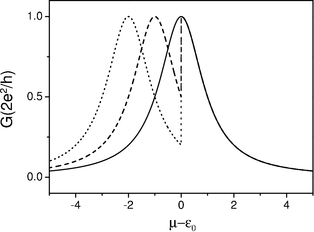
In the absence of interaction the conductance profile is a Lorentzian (solid line). If $U\neq 0$, when the Fermi energy crosses the BIC (in $\mu=\varepsilon_{0}$) the resonance shifts in $-U/2$, as shown for $U=2$ and $U=4$ (dash y dotted line, respectively). In other words, the sudden filling of a BIC, as described by Eq. (13), shifts the energy of the transmitting state, with the subsequent arising of a discontinuity in the conductance. This rough description allows to gain more insight of the results shown by Büsser et al. in multilevel quantum dots in Kondo regime [28]. These authors found similar discontinuities in the conductance as the gate voltage was varied, when a localized state crossed the Fermi energy. These localized states are a many-body version of the bound states in the continuum discussed here. This effect is analogous to that of a charge sensing described in [30], but in the present scheme, the sensed charge is that of a BIC inside the proper system.

In summary, we have studied the behavior of the Friedel phase in quantum dots systems when BICs are produced. This phase exhibits an abrupt change when these states arise, effect with consequences in the charge of the system, which jumps in a unity when the energy of the BIC drops below the Fermi energy.

References

- [1] J. von Neumann and E. Wigner, Phys. Z. 30, 465 (1929).
- [2] L. Fonda and R. G. Newton, Ann. Phys. 10, 490 (1960).
- [3] Frank H. Stillinger and David R. Herrick, Phys. Rev. A 11, 446 (1975).
- [4] H. Friedrich and D. Wintgen, Phys. Rev. A 31, 3964 (1985); H. Friedrich and D. Wintgen, Phys. Rev. A 32, 3231 (1985).
- [5] R. L. Schult, H. W. Wyld, and D. G. Ravenhall, Phys. Rev. B 41, 12760 (1990).
- [6] Zhen-Li Ji and Karl-Frederik Berggren, Phys. Rev. B 45, 6652 (1992).
- [7] M. L. Ladrón de Guevara, F. Claro, and P. A. Orellana, Phys. Rev. B 67, 195335 (2003).
- [8] I. Rotter and A. F. Sadreev, Phys. Rev. E 71, 046204 (2005).
- [9] G. Ordóñez, K. Na, S. Kim, Phys. Rev. A 73, 022113 (2006).
- [10] M. L. Ladrón de Guevara and P. A. Orellana, Phys. Rev. B 73, 205303 (2006).
- [11] A. F. Sadreev, E. N. Bulgakov and I. Rotter, Phys. Rev. B 73, 235342 (2006).
- [12] S. Longhi, Eur. Phys. J. B 57 45 (2007).
- [13] Federico Capasso, Carlo Sirtori, Jerome Faist, Deborah L. Sivico, Sung-Nee G. Chu and Alfred Y. Cho, Nature 358, 565 (1992).
- [14] J. S. Langer and V. Ambegaokar, Phys. Rev. 121, 1090 (1961).
- [15] Tooru Taniguchi and Markus Büttiker, Phys. Rev. B 60 13814 (1999).
- [16] D. C. Langreth, Phys. Rev. 150, 516 (1966).
- [17] H.-W. Lee, Phys. Rev. Lett. 82, 2358 (1999).
- [18] A. L. Yeyati and M. Büttiker, Phys. Rev. B 62, 7307 (2000).
- [19] S. Bandopadhyay and P. S. Deo, Phys. Rev. B 68, 113301 (2003).
- [20] M. Rontani, Phys. Rev. Lett. 97, 076801 (2006).
- [21] P. S. Deo, Phys. Rev. B 75, 235330 (2007).
- [22] Supriyo Datta and Weidong Tian, Phys. Rev. B 55, R1914 (1997).
- [23] E. Akkermans, A. Auerbach, J. E. Avron and B. Shapiro, Phys. Rev. Lett. 66 76 (1991).
- [24] V. A. Gopar, P. A. Mello, and M. Büttiker, Phys. Rev. Lett. 77, 3005 (1996).
- [25] Hongqi Xu and Weidong Sheng, Phys. Rev. B 57, 11903 (1998).
- [26] Tae-Suk Kim, Sam Young Cho, Chul Koo Kim, and Chang-Mo Ryu, Phys. Rev. B 65, 245307 (2002).
- [27] A. V. Malyshev, P. A. Orellana, F. Domínguez-Adame Phys. Rev. B 74, 033308 (2006).
- [28] C. A. Büsser, G. B. Martins, K. A. Al-Hassanieh, Adriana Moreo, and Elbio Dagotto, Phys. Rev. B 70, 245303 (2004).
- [29] D. S. Fisher and P. A. Lee, Phys. Rev. B 23, 6851 (1981).
- [30] R. Berkovits, F. von Oppen, and Y. Gefen, Phys. Rev. Lett. 94 076802 (2005).