On the theory of cavities with point-like perturbations. Part I: General theory
Abstract
The theoretical interpretation of measurements of “wavefunctions” and spectra in electromagnetic cavities excited by antennas is considered. Assuming that the characteristic wavelength of the field inside the cavity is much larger than the radius of the antenna, we describe antennas as “point-like perturbations”. This approach strongly simplifies the problem reducing the whole information on the antenna to four effective constants. In the framework of this approach we overcame the divergency of series of the phenomenological scattering theory and justify assumptions lying at the heart of “wavefunction measurements”. This selfconsistent approach allowed us to go beyond the one-pole approximation, in particular, to treat the experiments with degenerated states. The central idea of the approach is to introduce “renormalized” Green function, which contains the information on boundary reflections and has no singularity inside the cavity.
1 Introduction
Cylindrical microwave cavities with different cross-sections and small height are now widely used as the simplest realization of “quantum” (wave) billiards [1, 2, 3]. Indeed for the lowest TM-mode (transversal magnetic) inside of the cavity the transversal component of electric field satisfies the two-dimensional Helmholz equation with Dirichlet boundary condition [4]. This problem is mathematically equivalent to the problem for the quantum particle inside a box with hard walls. This boundary problem can not be solved analytically for arbitrary cavity shapes, where the corresponding classical problem is non-integrable and shows chaotic behavior. Microwave cavities are a simple realization of “quantum” chaotic systems. In spite of its experimental simplicity, microwave billiards exhibit general properties of quantum chaotic systems [5].
Experimentally the cavity is always open, since one has to excite and measure the field inside. Usually one antenna is used for an excitation and the same or a second one for the measurement [5] (see Fig.1). These antennas can be considered as “probes”, assuming that the influence of antennas on the investigated properties is comparatively small. However this assumption quite often is violated. To understand the data in these cases we have developed a self-consisted theory of the experiment.
The detailed analysis of the antenna construction represents an individual complicated problem [6]. Therefore one has to treat antennas phenomenologically to obtain analytical formulas. The standard scattering matrix formalism [7, 8, 5] applied to the billiard system does not take properly into account singularities from the sources and contains divergent series. This disadvantage can be overcome if one uses an approach based on “point perturbations” of the system [9, 10]. The main idea of the approach is the introduction of the “renormalized” Green function instead of the Green function with coincident space arguments.
In Section 2 we explain the idea of a point-like perturbation in two-dimensional case and derive the matching condition between wavefunctions inside of the antenna and inside of the cavity. Doing this we basically follow the line of Exner and eba [11]. Ibidem we discuss the physical meaning of the coupling coefficients. In Section 3 we generalize the scattering matrix (-matrix) obtained in [11] to the case of multiple antennas and estimate coupling coefficients for metallic and dielectric scatterers. Section 4 represents a general theory of an experimental wavefunction extraction based on the expression for -matrix obtained in the previous section. The theory is based on the one-pole approximation in the isolated resonances regime. At the end of the Section we show what happens when the “wavefunction” is measured in the case of degenerated states.
While for closed cavities one can take into account only a finite number of resonances inside of the experimental range of wavenumbers, for open cavities this approximation fails. In Section 5 we show that for an open cavity with broad resonances the transmission coefficient between two antennas is proportional to the Green function of the unperturbed system. This gives the possibility to investigate the spatial structure of the Green function of an open cavity, for example nodal domain distributions [12, 13].
2 Matching for point-like antenna
a)

b)

We now discuss the general idea of the approach used in Ref. [11] which allows us to treat the presence of scatterers and antennas in a simple way assuming that the wavelength of the field is much larger than the characteristic size of the area of the attachment. Figure 1 illustrates the principal setup to measure spectra of a cavity. One sees that a quasi-one dimensional waveguide is attached to a cavity at some point. We will assume that the waveguide is straight and one can separate variables inside of it and define a scalar longitudinal wavefunction depending on the variable inside the waveguide. Furthermore we assume that the height of the cavity is small and the distance between transversal wavenumbers is large. Thus it is natural to suppose that the one-dimensional longitudinal wavefunction in the waveguide relates to the longitudinal wavefunction in the cavity in such a way that only some general and energy independent properties of the matching are important. Since the detailed construction of the matching usually is quite complicated, the only restriction applied is that the final operator describing the coupling between antenna and cavity should be linear and Hermitian.
We substantially follow paper [11]. Basically the idea of the approach is to construct a self-adjoint extension of the Hamiltonian in the presence of point-like perturbations. In various situations self-adjoint extensions were considered [10, 14] and related problems were studied [15, 16].
Let us consider the matching of a quasi one-dimensional antenna to a cavity. We denote by the longitudinal wavefunction inside the one-dimensional antenna and by a function inside the cavity. Thus is a function on the space consisting of two parts: cavity and antenna. We assume that the antenna is coupled at the end to the point of the cavity. We define the operator which acts on the function in the following way:
| (1) |
where and is the two-dimensional Laplacian. Since for TEM-mode in the waveguide and the lowest TM-mode in the cavity thresholds do not exist we did not consider them in Eq. (1). The generalization to higher transversal modes in the cavity will be presented in the Section 7.
In the stationary case we look for the solution of the spectral problem
| (2) |
where is the total wavenumber.
Now we turn to the question how to define operator to be Hermitian. This is equivalent to the introduction of proper boundary matching conditions for the functions and .
In order to avoid divergent integrals at the origin first we consider the cavity with a small pricked ring of radius with a center at the point . We call this area . Following the general procedure [17, 9, 11] we consider two quadratic forms
| (3) |
where bar means complex conjugation, superscript ‘’ denotes hermitian conjugation and angle brackets mean integration. Then consider the difference
| (4) |
In the last equality we introduced cylindrical coordinates , , and assumed
| (5) |
where is the physical boundary of the cavity and is the derivative along the outer normal to the boundary. This is equivalent to the assumption that the functions or their normal derivatives are zero at the boundary (Dirichlet or Neumann boundary conditions or their linear combination).
Assuming that functions have the same kind of singularities for as the Green function for the two-dimensional plane [18, 19]
| (6) |
where is the Hankel function of the first kind and is Euler constant, we can write asymptotic expansions for :
| (7) |
where are constants. We have written the factor in order to simplify the further calculations. Here is calculated in arbitrary length units. Though depends on the choice of the length unit, the sum of the first two terms in expansions (7) is invariant. We will discuss this feature later.
Assuming that and for , we get
| (8) |
Finally in the limit equality (4) takes the form
| (9) |
Let us introduce vectors , , , and rewrite the last equality in the form
| (10) |
where denotes the scalar product of two vectors. Since the operator is linear we write
| (11) |
and get that matrix has to be Hermitian. Thus the general matching condition reads
| (12) |
where are real and . As it is assumed that is -independent, the constants and are -independent as well. From the last formula one can see that for antenna and cavity are decoupled, which means there is no mixing between functions : , . Thus we conclude that are coupling constants, describes the boundary condition at the end of the antenna and describes the scattering strength of the antenna. corresponds to (Dirichlet boundary condition) and corresponds to (Neumann boundary condition).
Let us now prove the invariance on the length scale of the expression (7). From the matching condition (12) we have
| (13) |
Substituting this relation in (7) we get
| (14) |
Let us introduce the scattering length by the following equality
| (15) |
Then (14) takes the form
| (16) |
which is invariant. The definition of the scattering length (15) corresponds to the condition that the wavefunction is zero at the distance from the perturbation point when . It differs from the definition given in [9].
3 -matrix for a cavity with multiple antennas
Here we consider the case with antennas attached to a cavity at points . We look for the solution in the form
| (17) |
where is the solution inside the -th antenna, is the field inside the cavity, is the Green function in the cavity and are unknown coefficients which have to be defined.
The Green function has singularities at the points . Thus in the neighborhood of we write
| (18) |
where represents the renormalized Green function. It plays the key role in the following calculations. Numerically the renormalized Green function can be calculated by means of the boundary element method [20].
From the definition we see that depends on the chosen system of units. However all equations determining physical observable quantities will of course be invariant.
Then we define generalized boundary values at the matching points
| (19) |
Using matching condition (12), we get
| (20) |
These equations can be rewritten in a matrix form
| (21) | |||
| (22) |
where vectors have elements respectively, matrix has elements
and diagonal matrices have elements on diagonals respectively. Substituting from (22) into (21) we get
| (26) |
where . Thus
| (27) |
where the -matrix has the form
| (28) |
The Green function of a closed cavity is real, thus from Eq. (28) one sees that the -matrix is unitary. Using the equality
| (29) |
we represent in the following way:
| (30) |
For the case of a single antenna formula (30) was obtained in [11].
From (30) we see that poles of -matrix are the complex solutions of the equation
| (31) |
In the limit of a closed system () we get the equation determining the spectrum of the system with only scatterers inside
| (32) |
Eq. (32) shows that in the limit , poles of the system approach the poles of the unperturbed system.
3.1 One-dimensional cavities
If an antenna is attached to a narrow waveguide with a width comparable to the wavelength, then the cavity can be considered as the one-dimensional one. The -matrix for such a cavity can be calculated analogously to two-dimensional case. We introduce the operator inside the cavity
| (33) |
where is a threshold from the quantization in direction. We are looking for the solution of the spectral problem (2). We denote the position of the antenna attachment, are the coordinates of the ends of the cavity, . Calculating the difference of two quadratic forms we get
| (34) |
where ,
| (35) |
Then we write . From (34) is Hermitian. Usually one assumes that , thus
| (36) |
This gives
| (37) | |||
| (38) |
For a cavity with a scatterer inside () we get
| (39) |
Exactly the same condition holds for the derivatives of the solution of the following equation with true delta-scatterers
| (40) |
We have mapped the problem of a 1D cavity with a point-like scatterer to a Schrödinger equation with a -potential. Such a mapping is possible in one-dimensional system only.
From the asymptotic
| (41) |
the condition (39) and the assumption that we find , where is a scattering length.
Let us now construct the -matrix for a number of antennas attached to a cavity at the points . Analogously to (17), (20) we write
| (42) |
where and
| (43) |
where is the Green function of the closed one dimensional cavity. Using the identity
| (44) |
we find analogously to (30)
| (45) |
where
| (46) |
On the contrary to (32) poles of the closed system () tend to the unperturbed ones when .
3.2 Example: Single antenna attached to an infinite cavity
One can imagine a Gedankexperiment where an antenna is attached to an infinitely large cavity. In such a cavity there are no reflections from the walls. Experimentally this situation can be realized if one places a perfect absorber along the boundary of the cavity. In terms of the cross-section such a resonator can be considered as a two-dimensional plane.
Let us consider a single antenna attached to a plane at the point . In this case the unique element of -matrix is equal to the reflection coefficient and are scalar constants. From (30) we find
| (47) |
where
| (48) |
The last equality follows from (6). In the limit of a closed cavity the pole of is
| (49) |
where is the scattering length. The eigenvalue of the problem (2) is . This eigenvalue corresponds to the eigenstate induced by a point-like scatterer with a wavenumber below the threshold. This means that a point-like scatterer in two-dimensional case can be always treated “quantum-mechanically” as an attractive well. Since in electromagnetic cavities the threshold for the lowest transversal mode is equal to zero, this pole can be observed only for higher transversal modes.
3.3 Estimation of the scattering length
In the previous example we showed that a point-like perturbation can be always treated as an attractive well. Nevertheless using it one can model not only dielectric but also metallic scatterers. The apparent contradiction is explained by the fact that in the long-wave limit the whole information about the scatterer is reduced to its scattering length which can be the same for the attractive as well as for the repulsive scatterer. This description fails whenever two scatterers are close to each other or close to the boundary (compare [21]). Below we estimate a scattering length for attractive and repulsive scatterers.
Let us consider a cylindrical cavity with radius and a cylindrically symmetric scatterer of radius whose center coincides with the centrum of the cavity. We shall treat the scatterer in a quantum-mechanical way as a potential and shall consider states with zero angular momentum.
We put the origin of the frame in the center of the cavity. We denote the wavefunctions inside and outside of the scatterer by and , respectively. Here . Then
| (50) |
where and are Bessel and Neumann functions of zero order. At the boundary of the cavity . This gives . Equating logarithmic derivatives at the boundary of the scatterer we find
| (51) |
where . We assume that . Then one can put on the left hand-side of (51) and use the asymptotic expansions , , , [19]. This gives
| (52) |
From the last equation we get the condition
| (53) |
Let us consider what happens if we simulate the scatterer by a point-like perturbation. Using the following equalities
| (54) |
| (55) |
This gives the following quantization condition
| (56) |
Comparing Eqs. (53) and (56) we find
| (57) |
Let us discuss the last result. First it shows that a singular point-like scatterer can model an attractive as well as a metallic scatterer. For the metallic scatterer of the radius we find and in accordance with (16).
Let us consider now an “attractive scatterer”. For simplicity we consider a potential well of constant depth . Then , , . If then
| (58) |
Substituting (58) in (57) we find that the scattering length can increase exponentially for an attractive scatterer. For quite small we have . Thus we conclude that exponential increase of the scattering length for an attractive scatterer leads to the new characteristic length different from the radius of the scatterer.
From (55) we find that the cases of small “metallic” scatterers () and small attractive (“dielectric”) scatterers () lead to different signs of the shift of resonances of the resonator with respect to the empty one. For metallic scatterers resonances are shifted to higher wavenumbers and for the dielectric ones they are shifted to lower wavenumbers (see also [5]), which will become evident from the next section.
4 Wavefunction measurements
In this section we consider the technique of wavefunctions measurements in the closed cavity. If the cavity is closed, its spectrum is discrete. The presence of antennas opens the cavity, thus all eigenvalues become resonances of the -matrix. If some resonances are isolated from the rest, they can be considered separately and the influence of all others can be neglected. The same consideration takes place for an open cavity with a number of sharp resonances, isolated from the rest. The wavefunction corresponding to an isolated sharp resonance can be measured experimentally. Below we consider the idea of wavefunction measurements and some effects appearing if resonances are overlapping.

4.1 One pole approximation
Close to an eigenvalue of the discrete spectrum the Green function may be written as
| (59) |
provided and are far enough from each other. Function can be written in the form
| (60) |
where has no pole at . In one pole approximation (60) reads
| (61) |
Using (59), (61) one can calculate the inverse matrix appearing in Eq. (30) [2]. Indeed in this case
| (62) |
where , , , with the renormalized dimensionless coefficient
| (63) |
Using the identity
| (64) |
we can rewrite Eq. (30) for close to in the form
| (65) |
where . This immediately gives us poles of the -matrix:
| (66) |
Since nondiagonal elements are proportional to , they contain an additional information on the sign of the wavefunction.
Formula (66) implies the possibility to measure wavefunctions through the shifts of resonances at different points of the cavity induced by a point like perturbation. In Ref. [1] the author used a movable point-like scatterer and fixed antenna whereas in [2, 22] the antenna has been moved.
Figure 2 illustrates shifts of the resonance of the empty rectangular cavity (solid curve) as well as in the presence of a small metallic (dashed curve) and a dielectric (dashed-dotted curve). One sees that for a metallic scatterer the resonance is shifted to a higher wavenumber11 1 For the larger metallic scatterer ( mm) we observed a shift of the resonances to the lower wavenumbers in the low- regime (). This might be related to the fact that in the lower wavenumbers regime the distance between antenna and scatterer becomes comparable to the wavelength and the scattering length of the antenna. Then the proper description of the situation requires to go beyond one-pole approximation or even beyond the concept of a point-like scatterer. This experiment has to be investigated further in details. while for the dielectric scatterer it is shifted to a lower wavenumber. This observation is in agreement with the arguments of the Section 3.3.
4.2 -poles approximation
In -poles approximation one takes into account only contributions from poles in some range of wavenumbers. For we get an approximate expression for the Green function truncating the convergent series at the th term:
| (67) |
can be written in the form
| (68) |
where has no poles for . The approximation assumes that the energy dependence of can be neglected. Then we get approximately
| (69) |
where is some value from the range . Using (67), (69) we can write
| (70) |
Here , , , . We see that inside of the given window of wavenumbers is an offset renormalizing the scattering strength.
Let us write -matrix (30) in -poles approximation. We neglect energy dependence everywhere apart from the Green function. We have
| (71) |
where , . We write
| (72) | |||
| (73) |
Finally we get
| (74) | |||
| (75) |
If then
| (76) |
Introducing an effective Hamiltonian
| (77) |
we can write
| (78) |
Experimentally one usually removes the global phase of -matrix, describing the antenna matching itself. Theoretically this means that instead of (78) one introduces a new matrix
| (79) |
Poles of -matrix can be found from the equation
| (80) |
For the closed system the last equation reduces to
| (81) |
Effective Hamiltonians of the type (77) were used in [5, 7, 8]. Resonances of -matrix in a general situation are discussed in [23].
4.3 Experimental “wavefunctions” in the case of degenerated states
Let us consider a cavity with the degenerated eigenvalue . In this case any weak perturbation mixes all eigenstates corresponding to . In the wavefunction measurement an antenna is a perturbation. Moving the antenna one changes mixing coefficients and produces a new field configuration inside the cavity. Therefore it is not clear whether one can easily treat the experimental wavefunction in this case. We show below that the experimental pattern in such a situation is just a sum of squares of all eigenfunctions . This combination is invariant with respect to the choice of eigenfunctions.
The simplest approximation in this situation is to take into account only eigenfunctions corresponding to . Let us calculate an experimental pattern which can be reconstructed from the measurement with a single antenna. The resonance position for the fixed antenna position R can be calculated from Eq. (80). Using Eq. (69) we get
| (82) | |||
| (83) |
From Eq. (83) we conclude that in the case of degenerated eigenvalue the experimentally measured pattern should correspond to the sum of squares of corresponding eigenfunctions.
In Fig. 3 experimental examples from a rectangular microwave billiard with a side ratio of 2:1 are presented. For the technical details the reader is referred to Ref. [24]. The figure shows experimental and theoretical patterns corresponding to doublets consisting of the th, th states and the th, th states. States of each doublet are degenerated, the data were obtained from the reflection measurement with a single movable antenna. Thus one expects to measure the sum of squares of two eigenfunctions. Pictures a)-d) illustrate experimental data, all others show theoretical simulations.
a)

c)

e)

g)

i)

b)

d)

f)

h)

j)

Fig. 3a) shows the resonances corresponding to the th state with the antenna at the positions marked by a square, a triangle and a disk at Fig. 3c). Solid, dashed and dashed-dotted lines in Fig. 3a) correspond to a square, a triangle and a disk, respectively. Here only a single resonance is observed and no splitting could be seen. Fig. 3b) shows the shift of the resonance while the antenna is shifted along the horizontal line in Fig. 3c). In Figs. 3c) and d) the obtained resonance wavenumber shifts patterns are plotted in a gray-scale. In Figs. 3e)-h) the squares , of the rectangular eigenstates are plotted. In Figs. 3i)-j) is plotted, demonstrating the perfect agreement with the experimental results shown in Figs. 3c)-d).
5 Transmission measurements in open systems
Recent measurements of nodal domains in open microwave cavities [12, 13] raised a question on the theoretical description of this type of experiments. The crucial difference compared to the case considered above of a closed cavity consists in the absence of sharp resonances of the -matrix. This makes it impossible to use the one-pole approximation being the base of wavefunctions measurements in closed systems.
In the experiment the transmission coefficient from the fixed antenna to the movable one is measured and interpreted directly as a “wavefunction” corresponding to the continuous spectrum of the unperturbed open system. We show below that in fact in the experiment the Green function of the cavity is measured. To prove this statement we start from Eq. (30). The straightforward calculation gives for the case of two antennas
| (84) | |||
| (85) |
Let us assume that is far from all poles and scattering is weak, i.e.
| (86) |
Here we used (15). Thus for quite distant antennas we can write
| (87) |
Measuring at a fixed wavenumber and a fixed antenna position we get a value proportional to . An additional phase shift in due to the prefactor of the Green function in Eq. (84) can be easily removed for the closed cavity, since the Green function in this case is real.
5.1 Example: Single antenna attached to a semi-infinite cavity
The following example illustrates general effects taking place in the vicinity of a boundary. We consider two antennas attached to a semi-infinite cavity at points . The cross-section of the cavity is a half plane.
Let the boundary of the cavity coincides with -axis in the plane. We define . The transmission coefficient through these antennas is defined by (84) where can be found from the method of images:
| (88) |
| (89) |
For simplicity we assume and neglect nondiagonal elements in in (85). In this approximation
| (90) |
If the movable antenna is placed far from the boundary then . Using the asymptotic expansion of the Hankel function [19] and (15) we write
| (91) |
Thus we see that at distances of the order of the wavelength from the boundary contains an oscillating term. This term decays when one moves the antenna away from the boundary. The origin of this oscillating part is the mirror source of the movable antenna. This mirror source can be treated as an “impurity” charge, thus the oscillating behavior of may be interpreted in terms of Friedel oscillations [25].
6 Cavity with closed loops
In this section we consider a cavity with closed loops (see Figure 4). This model is another realization of a quantum graph [26]. In order to simplify calculations we do not consider attached antennas.

6.1 Cavity with short loops
Analogously to Eq. (1) we introduce the Hamiltonian inside the cavity
| (93) |
Repeating steps (3)-(10) we get
| (94) |
where are vectors with components , .
6.2 A more realistic model of the loop
The model of loops considered above is appropriate only for short loops or for some narrow energy region since it does not contain the spectrum of the one-dimensional wire connecting different points. To take into account the “inner structure” of the loop let us consider a more realistic model. We consider a cavity with a loop of the length matched to it at two points . We neglect the curvature of the wire. Analogously to Eq. (17) we write
| (99) |
Matching conditions (12) at points give
From Eq. (6.2) we find that the spectrum of the system is defined by the equation
| (114) |
where are matrices
If the cavity and the wire are decoupled then and Eq. (114) reduces to
| (121) |
The last equation gives the unification of spectra of the cavity with scatterers inside and the wire.
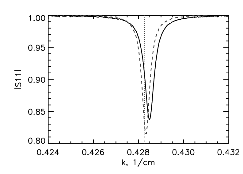
In Fig. 5 one sees the experimentally observed shift of the same resonance of the rectangular cavity as shown in Fig. 2. The dotted line shows the position of the eigenwavenumber of the rectangular cavity. The solid line corresponds to the modulus of the reflection coefficient from the cavity excited by the antenna with two additionally attached antennas each closed by a 50 load. The dashed line illustrates the modulus of the reflection coefficient from the same cavity, were the antennas were connected by a wire.
7 The -matrix for multimode cavity
If there are more than one open transversal modes in the cavity with transversal wavenumbers the ansatz of the solution (17) has to be generalized. To treat this situation let us consider identical “copies” of the cavity (see figure 6) with wavefunctions and introduce the operator acting on the spacial variables of the antenna and the cavities:
| (122) |
where is -th transversal wavenumber.

We look for the solution of the spectral problem (2) in the form
| (123) |
where (for the lowest TM-mode in electromagnetic billiards and ).
The same procedure as for a single transversal channel gives us the following expression for the -matrix:
| (124) |
where , ,
| (125) |
Here the matrix has elements
| (126) |
where .
8 Conclusions
In the paper we presented the general selfconsistent theory for measurements on electromagnetic cavities with point-like antennas and scatterers. In the framework of the considered approach we justified the idea lying on the heart of wavefunctions measurement. The experimental patterns for the cases of degenerated states are explained. The generalization of the basic idea allowed to describe cavities with more than one open transversal channel and antennas connected by loops. Mathematical objects appearing in the last cases can be considered as quantum graphs.
9 Acknowledgements
We gratefully acknowledge useful discussions with Petr eba. This work was supported by the Deutsche Forschungsgemeinschaft via an individual grant.
Appendix A Operator algebra for point scatterers in a closed cavity.
Similar to the one-dimensional case one usually treats a point-like scatterer as a -potential which can be written in an arbitrary representation as a matrix , where is a coupling matrix [5]. However in a multidimensional case a point-like perturbation does not correspond exactly to a -potential. We show below that instead of a -potential in the two-dimensional case a point-like scatterer situated at the point R is described by a product , where is a renormalizing operator.
From Eqs. (7), (19) we find that the function obeys the equation
| (127) |
Using Eq. (12) with we write
| (128) |
where
| (129) |
Thus acts on the function without a singularity at the point as an identical operator and gives the renormalized value for a function with a logarithmic singularity (see Eq. (7)).
In the basis of eigenfunctions the matrix elements of the -function are given by
| (130) |
In this basis Eq. (128) reads
| (131) |
where , . The solvability condition of Eq. (128) is
| (132) |
The last equality can be rewritten in the form
| (133) |
For any vectors we have if exists. Thus for we have
| (134) |
From this we conclude that
| (135) |
Finally the equation for the spectrum reads
| (136) |
The last equation is in accordance with (32).
Appendix B Green function for the system with antennas.
Let us consider a cavity with a number of fixed antennas. In order to measure the wavefunction of such a system one has to introduce a movable antenna. The wavefunction of the cavity with a movable antenna is the Green function of the cavity with only fixed antennas. Then the natural question is to calculate Green function of the cavity with a number of fixed antennas.
Let us look for the Green function of the system with fixed antennas in the form
| (137) |
where is the Green function for the cavity without antennas. The function (137) satisfies the equation for the Green function. The Green function should correspond to outgoing waves spreading inside of the fixed antennas, thus inside of the th fixed antenna the solution is
| (138) |
In the neighborhood of the Green function has the following asymptotic
| (139) |
Using the condition (12) we get
From the last equality analogously to (21), (22) we find
| (147) |
If then the last formula reduces to the so-called “Krein’s resolvent formula” for the Green function of the system with point-like scatterers [10]. Krein’s formula can be also obtained by the operator technic of Appendix 1 using the following identities
| (148) |
where .
References
- [1] S. Sridhar. Experimental observation of scarred eigenfunctions of chaotic microwave cavities. Phys. Rev. Lett., 67:785, 1991.
- [2] J. Stein, H.-J. Stöckmann, and U. Stoffregen. Microwave studies of billiard Green functions and propagators. Phys. Rev. Lett., 75:53, 1995.
- [3] U. Kuhl, H.-J. Stöckmann, and W. Weaver. Classical wave experiments on chaotic scattering. J. Phys. A, 38:10433, 2005.
- [4] J. D. Jackson. Classical Electrodynamics. Wiley, New York, 1962.
- [5] H.-J. Stöckmann. Quantum Chaos - An Introduction. University Press, Cambridge, 1999.
- [6] J. Barthélemy. Chaos Ondulatoire en Presénce de Pertes: Modélisation et Expérience de Billards Micro-Ondes. PhD thesis, Université Paris, 2003.
- [7] C. Mahaux and H. A. Weidenmüller. Shell-Model Approach to Nuclear Reactions. North-Holland, Amsterdam, 1969.
- [8] C. H. Lewenkopf and H. A. Weidenmüller. Stochastic versus semiclassical approach to quantum chaotic scattering. Ann. Phys. (N.Y.), 212:53, 1991.
- [9] Yu. N. Demkov and V. N. Ostrovskiy. Zero-range potentials and their applications in atomic physics. Plenum Press, New York, 1988.
- [10] S. Albeverio, F. Gesztesy, R. Høegh-Krohn, and H. Holden. Solvable Models in Quantum Mechanics. Springer, New YorkBerlin, 1988.
- [11] P. Exner and P. eba. Resonance statistics in a microwave cavity with a thin antenna. Phys. Lett. A, 228:146, 1997.
- [12] U. Kuhl, R. Höhmann, H.-J. Stöckmann, and S. Gnutzmann. Nodal domains in open microwave systems. Phys. Rev. E, 75:036204, 2007.
- [13] U. Kuhl. Wave functions, nodal domains, flow, and vortices in open microwave systems. Eur. Phys. J. Special Topics, 145:103, 2007.
- [14] B. L. Voronov, D. M. Gitman, and I. V. Tyutin. Self-adjoint differential operators assosiated with self-adjoint differential expressions. Preprint, 2006. quant-ph/0603187v2.
- [15] S. Albeverio, F. Haake, P. Kurasov, M. Kuś, and P. Šeba. S-matrix, resonances, and wave functions for transport through billiards with leads. J. Math. Phys., 37:4888, 1996.
- [16] J. Brüning and V. A. Geyler. Scattering on compact manifolds with infinitely thin horns. J. Math. Phys., 44:371, 2003.
- [17] L. D. Landau and E. M. Lifshitz. Quantum Mechanics: (Nonrelativistic Theory). In: Theoretical Physics 3. Pergamon Press, Oxford, London, Edinburgh, 1965.
- [18] Dean G. Duffy. Green’s functions with applications. Chapman & Hall/CRC, Boca Raton, 2001.
- [19] I. S. Gradshteyn and I. M. Ryzhik. Table of Integrals, Series, and Products. Corrected and enlarged edition. Academic Press, San Diego, 1980.
- [20] Shuichi Tasaki, Takahisa Harayama, and Akira Shudo. Interior dirichlet eigenvalue problem, exterior neumann scattering problem, and boundary element method for quantum billiards. Phys. Rev. E, 56, 1997.
- [21] J. Brüning, S. Yu. Dobrokhotov, V. A. Geyler, and T. Ya. Tudorovskiy. On the theory of multiple scattering of waves and the optical potential for a system of point-like scatterers. An application to the theory of ultracold neutrons. Russ. J. Math. Phys., 12:157, 2005.
- [22] J. Stein and H.-J. Stöckmann. Experimental determination of billiard wave functions. Phys. Rev. Lett., 68:2867, 1992.
- [23] I. Rotter. Dynamics of quantum systems. Phys. Rev. E, 64:036213, 2001.
- [24] U. Kuhl, E. Persson, M. Barth, and H.-J. Stöckmann. Mixing of wavefunctions in rectangular microwave billiards. Eur. Phys. J. B, 17:253, 2000.
- [25] Arnd Bäcker, Thomas Friedrich, Maksim Miski-Oglu, Achim Richter, and Steven L. Tomsovic. Friedel oscillations in microwave billiards. private communication, 2008.
- [26] T. Kottos and U. Smilansky. Quantum graphs: a simple model for chaotic scattering. J. Phys. A, 36:3501, 2003.