Nested Cluster Algorithm for Frustrated Quantum Antiferromagnets
Abstract
Simulations of frustrated quantum antiferromagnets suffer from a severe sign problem. We solve the ergodicity problem of the loop-cluster algorithm in a natural way and apply a powerful strategy to address the sign problem. For the spin Heisenberg antiferromagnet on a kagomé and on a frustrated square lattice, a nested cluster algorithm eliminates the sign problem for large systems. The method is applicable to general lattice geometries but limited to moderate temperatures.
pacs
75.10Jm, 75.40Mg, 75.50.EeMonte Carlo calculations are a powerful tool for first principles investigations of strongly coupled quantum systems. Early simulations of quantum spin systems were performed with local Metropolis-type algorithms [1]. They suffered from critical slowing down and were thus limited to rather high temperatures. Cluster algorithms perform non-local updates and are capable of substantially reducing critical slowing down. Such algorithms were first developed by Swendsen and Wang for discrete classical Ising and Potts spins [2] and then generalized by Wolff [3] to classical spins with a continuous symmetry. Improved estimators which average over an exponentially large number of configurations at polynomial cost are an additional benefit of cluster algorithms. The first cluster algorithm for the spin quantum Heisenberg model was developed in [4]. While that algorithm works efficiently only for quantum spin chains, the loop-cluster algorithm [5] is efficient also in higher dimensions, and was first applied to the 2-d spin Heisenberg antiferromagnet on a square lattice in [6]. The continuous-time variant of the algorithm eliminates the Suzuki-Trotter time-discretization error and can reach very low temperatures [7]. This method has also been used to simulate systems on very large lattices [8] and with very long correlation lengths [9]. An elegant and powerful related method based on stochastic series expansion is available as well [10].
Unfortunately, in many cases of physical interest, including frustrated quantum spin systems, quantum Monte Carlo calculations suffer from a very severe sign problem. Using an improved estimator, the sign problem of the 2-d classical model at vacuum angle has been addressed with a variant of the Wolff cluster algorithm [11]. In that case, some clusters are half-instantons also known as merons. Flipping a meron-cluster leads to a sign-change of the Boltzmann weight and hence to an exact cancellation between two configurations. As a consequence, only configurations without meron-clusters contribute to the partition function. Restricting the simulation to those configurations eliminates the sign problem, since all configurations in the zero-meron sector have a positive sign. The meron concept has been generalized to fermionic systems [12] and the meron-cluster algorithm has been used to solve a number of very severe fermion sign problems [13, 14, 15]. Unfortunately, the meron-cluster algorithm is not generally applicable. In fact, as shown in [16], some sign problems are NP-complete. Hence, a hypothetical method that can solve any sign problem would solve all NP-complete problems in polynomial time. This would imply the equality of the complexity classes NPP. Since it is generally believed that NPP, it is expected that a universally applicable method that solves all sign problems cannot exist. In this paper we construct a nested cluster algorithm which, for the first time, is capable of eliminating severe sign problems of frustrated antiferromagnets at least at moderate temperatures.
Let us consider the antiferromagnetic spin quantum Heisenberg model with the Hamiltonian
| (1) |
Here is a quantum spin operator located at the site of a lattice , and is the antiferromagnetic exchange coupling between a pair of spins located at the sites and . Although our method can be applied directly in the Euclidean time continuum, in order to ease its implementation we work in discrete time. Depending on the lattice geometry, the Hamiltonian is expressed as a sum of terms which leads to a Suzuki-Trotter decomposition of the partition function
| (2) | |||||
Here the inverse temperature represents the extent of a periodic Euclidean time interval, which is divided into discrete time steps of size . Each is a sum of mutually commuting pair interactions on a set of disconnected bonds. Inserting complete sets of spin states between the factors in eq.(2), the partition function is expressed as a path integral over all spin configurations [6]
| (3) |
The weight of a configuration is a product of contributions from individual space-time plaquettes corresponding to the two-spin transfer matrix elements . In the basis , , , , up to an irrelevant overall factor, the two-spin transfer matrix takes the form
| (4) |
with and . The off-diagonal transfer matrix elements are negative. The product of the negative signs over all space-time plaquettes defines the total of a spin configuration. The remaining factor represents a positive Boltzmann weight which can be interpreted as a probability and thus can be used for importance-sampling in a Monte Carlo simulation.
When one samples the system using the positive weight , one must include in the measured observables and expectation values are given by
| (5) |
Here the index refers to expectation values in the simulated ensemble with positive Boltzmann weights and partition function such that
| (6) | |||||
Here is the spatial volume and is the difference between the free energy densities of the original ensemble with the weight and the simulated ensemble with the positive weight . The expectation value of the sign is exponentially small in the space-time volume . Since it is obtained as a Monte Carlo average of contributions , one needs an exponentially large statistics in order to accurately measure . This is impossible in practice and gives rise to a very severe sign problem.
How can one increase the statistics by an exponential factor without investing more than a polynomial numerical effort? The meron-cluster algorithm [11, 12] achieves this by constructing an improved estimator for the sign. Like the meron-cluster algorithm, the method presented here is based on the loop-cluster algorithm [5] which decorates a spin configuration with bonds connecting spins to closed loop-clusters. The four spins on a space-time plaquette are connected in pairs. In fact, and in eq.(4) represent weights of two possible bond configurations on a space-time plaquette. The weight corresponds to bonds connecting the spins and with their time-like neighbors and , while corresponds to space-like bonds connecting with and with . Sites connected by bonds form a closed oriented loop-cluster. Up to an overall spin-flip of the entire cluster, the spin configuration on a cluster is determined by the cluster geometry. Time-like bonds connect parallel spins, while space-like bonds connect anti-parallel spins. Integrating out the spins, the partition function can be expressed as a sum over bond configurations
| (7) |
Here is the number of time-like and is the number of space-like plaquette break-ups, while is the number of loop-clusters. The factor arises because each cluster has two possible spin orientations. The partition function can be sampled by a Metropolis update of the plaquette break-ups. Remarkably, while the original cluster algorithm which operates on spins and bonds never changes the sign and is thus not ergodic [17], the algorithm which operates only on bonds (after the spins have been integrated out) is ergodic and still avoids unnatural freezing. Interestingly, remains invariant under cluster flips, i.e. all clusters are non-merons. However, in this case the meron-cluster algorithm does not solve the sign problem because almost half of the configurations in the zero-meron sector have a negative sign [17]. Since it does not change under spin flips, is uniquely determined by the bond configuration. It is important to note that the sign can be expressed as a product of cluster signs . Depending on the orientation of a cluster, each space-like break-up contributes a factor to the two clusters traversing the corresponding space-time plaquette. By construction, each cluster traverses an even number of space-like break-ups, and hence .
We distinguish space-time plaquettes shared by two different clusters from internal plaquettes belonging entirely to one cluster. Updating the break-up on a space-time plaquette shared by two different clusters does not lead to a sign-change. Only updates of cluster-internal plaquettes may change the sign. We apply the following method to construct an improved estimator for the sign. Once a statistically independent bond configuration has been produced by the cluster algorithm, we perform an inner Monte Carlo simulation by updating only the cluster-internal plaquette break-ups. Each cluster defines the set of lattice sites contained in . The inner Monte Carlo algorithm generates clusters with different orientations that visit all sites of in different orders, thus contributing different values of . In this process, break-ups that lead to the decomposition of into separate clusters must be rejected. The inner Monte Carlo algorithm estimates an average for each set of sites . Since the different sets are independent, the improved estimator of the sign is given by
| (8) |
Remarkably, the nesting of an outer and an inner cluster algorithm achieves exponential error reduction at polynomial cost. A similar strategy was very successfully applied to the measurement of exponentially suppressed Wilson loops in lattice gauge theory [18] as well as to quantum impurity models [19]. Correlation functions and susceptibilities can also be measured with improved estimators. Let us consider the staggered magnetization operator . Here is a stagger factor depending on the sub-lattice to which the site belongs. The corresponding staggered susceptibility
| (9) |
is obtained from an improved estimator which is given in terms of with as
| (10) |
In which cases will the nested cluster algorithm eliminate or at least substantially reduce the sign problem? Since some sign problems are NP-hard, it is expected that any method will fail at least in those cases. The nested cluster algorithm fails to solve the sign problem when a cluster fills almost the entire volume, because then the inner Monte Carlo algorithm becomes inefficient. Since large clusters necessarily arise in the presence of large correlation lengths, the nested cluster algorithm does not work efficiently in low-temperature ordered phases.
Even in the absence of long-range order, cluster algorithms may become inefficient if the clusters grow to unphysically large sizes beyond the physical correlation length. This potential problem is prevented when there is a reference configuration that limits cluster growth [15]. For the antiferromagnet on the square lattice the reference configuration is given by the classical Néel state, i.e. all spins in a loop-cluster are in a staggered pattern. The cluster-size squared is then tied to the staggered susceptibility which protects the clusters from growing to unphysically large sizes. Also for frustrated systems it is natural to consider a classical ground state as a reference configuration. When one quantizes the spins along a local quantization axis in the direction of the spin orientation in the classical ground state, an interesting algorithm with open string-clusters emerges. The spins in each cluster are in the reference configuration and hence these clusters are protected from becoming unphysically large. However, the meron-concept does not apply to the open string-clusters, i.e. when these clusters are flipped, they are not independent but affect each other in their effect on the sign. Remarkably, one can still integrate out the spins analytically. This glues the open string-clusters together to the closed loop-clusters of the algorithm discussed before. While typical closed loop-clusters are hence larger than the correlation length corresponding to the classical order, they still represent physical correlated regions. In fact, they grow up to the length scale at which the signs, which are a manifestation of quantum entanglement, decorrelate.
Even if the typical cluster-size is moderate, the inner Monte Carlo algorithm may not lead to an efficient cancellation of signs. For example, there are cases in which the improved estimator is not positive. Still, if such cases are rare, the sign problem is substantially reduced. In order to optimize the performance of the algorithm, the numerical effort invested in the inner and outer Monte Carlo procedures must be properly balanced against each other. It pays off to invest a larger number of inner Monte Carlo sweeps on the larger sets . In any case, the efficiency of the nested cluster algorithm must be investigated on a case by case basis.
We now consider the Heisenberg antiferromagnet with uniform nearest-neighbor coupling on the lattices illustrated in figure 1. The frustrated square lattice has an additional coupling along the diagonals.

We have simulated large kagomé lattices with up to spins at moderate temperatures with . Figure 2 shows the probability distribution of the improved estimator . Although sometimes it is negative, it still leads to an accurate determination of the average sign.

We consider with on sub-lattice , respectively, which may signal coplanar spin order. As shown in figure 3, with increasing volume both and decrease dramatically over numerous orders of magnitude, but are still accurately accounted for by the nested cluster algorithm. For example, with spins . A brute force approach would require an astronomical statistics of about sweeps in order to achieve a similar precision.
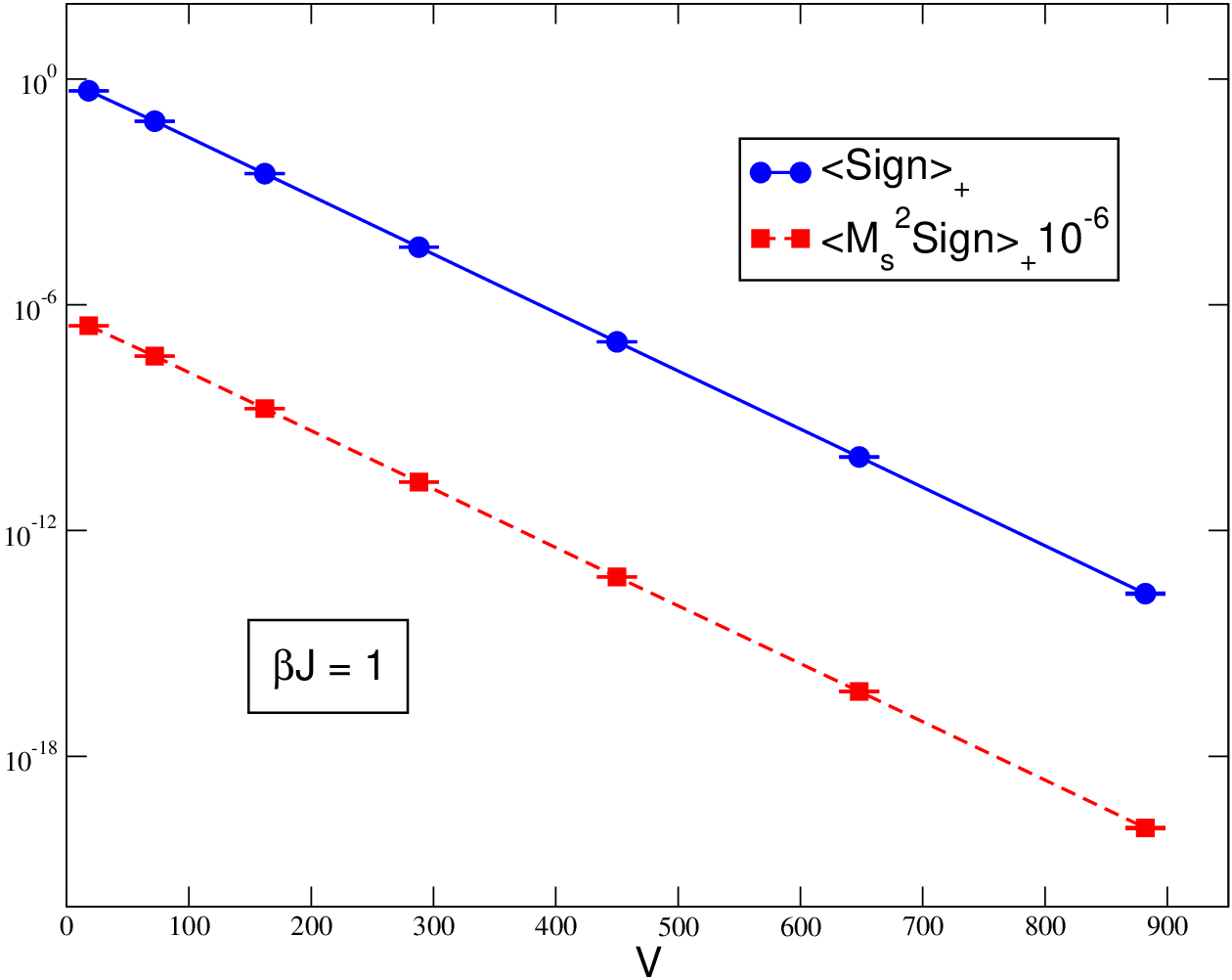
Figure 4 shows the coplanar staggered susceptibility compared to the collinear Néel susceptibility . On the square lattice, frustration reduces the Néel order, while (at least for ) the coplanar order is as weak as on the kagomé lattice (and practically indistinguishable from it in figure 4).

To conclude, in contrast to other Monte Carlo methods, the nested cluster algorithm is capable of eliminating very severe sign problems for large systems, at least at moderate temperatures. This is useful, for example, for determining the couplings of frustrated magnets by comparison with experimental finite temperature data. As we have demonstrated, although the nested cluster algorithm cannot reach very low temperatures, by studying appropriate susceptibilities one may still obtain valuable insights concerning possible types of order. Applications to frustrated antiferromagnets on various lattice geometries are currently in progress.
U.-J. W. likes to thank S. Chandrasekharan for a long-lasting fruitful and very inspiring collaboration on the sign problem. We also have benefited from interesting discussions with M. Troyer. This work was supported by the Schweizerischer Nationalfonds.
References
- [1] J. D. Reger and A. P. Young, Phys. Rev. B37 (1988) 5978.
- [2] R. H. Swendsen and J.-S. Wang, Phys. Rev. Lett. 58 (1987) 86.
- [3] U. Wolff, Phys. Rev. Lett. 62 (1989) 361.
- [4] U.-J. Wiese and H.-P. Ying, Phys. Lett. A168 (1992) 143.
- [5] H. G. Evertz, G. Lana, and M. Marcu, Phys. Rev. Lett. 70 (1993) 875.
- [6] U.-J. Wiese and H.-P. Ying, Z. Phys. B93 (1994) 147.
- [7] B. B. Beard and U.-J. Wiese, Phys. Rev. Lett. 77 (1996) 5130.
- [8] J.-K. Kim and M. Troyer, Phys. Rev. Lett. 80 (1998) 2705.
- [9] B. B. Beard, R. J. Birgeneau, M. Greven, and U.-J. Wiese, Phys. Rev. Lett. 80 (1998) 1742.
- [10] A. W. Sandvik, Phys. Rev. B56 (1997) 11678.
- [11] W. Bietenholz, A. Pochinsky, and U.-J. Wiese, Phys. Rev. Lett. 75 (1995) 4524.
- [12] S. Chandrasekharan and U.-J. Wiese, Phys. Rev. Lett. 83 (1999) 3116.
- [13] S. Chandrasekharan, J. Cox, K. Holland, and U.-J. Wiese, Nucl. Phys. B576 (2000) 481.
- [14] S. Chandrasekharan and J. C. Osborn, Phys. Rev. B66 (2002) 045113.
- [15] S. Chandrasekharan, J. Cox, J. C. Osborn, and U.-J. Wiese, Nucl. Phys. B673 [FS] (2003) 405.
- [16] M. Troyer and U.-J. Wiese, Phys. Rev. Lett. 94 (2005) 170201.
- [17] P. Henelius and A. W. Sandvik, Phys. Rev. B62 (2000) 1102.
- [18] M. Lüscher and P. Weisz, JHEP 09 (2001) 010.
- [19] J. Yoo, S. Chandrasekharan, and H. U. Baranger, Phys. Rev. E71 (2005) 036708.