Resonant interactions of nonlinear water waves in a finite basin
Abstract
We study exact four-wave resonances among gravity water waves in a square box with periodic boundary conditions. We show that these resonant quartets are linked with each other by shared Fourier modes in such a way that they form independent clusters. These clusters can be formed by two types of quartets: (1) angle-resonances which cannot directly cascade energy but which can redistribute it among the initially excited modes and (2) scale-resonances which are much more rare but which are the only ones that can transfer energy between different scales. We find such resonant quartets and their clusters numerically on the set of 1000 x 1000 modes, classify and quantify them and discuss consequences of the obtained cluster structure for the wavefield evolution. Finite box effects and associated resonant interaction among discrete wave modes appear to be important in most numerical and laboratory experiments on the deep water gravity waves, and our work is aimed at aiding the interpretation of the experimental and numerical data.
pacs
47.35.Bb, 89.75.KdI Introduction
Weakly nonlinear systems of random waves are usually studied in the framework of wave turbulence theory (WTT) (for introduction to WTT see book [1]). Besides weak nonlinearity and phase randomness, this statistical description is based on the infinite-box limit. This approach yields wave kinetic equations for the wave spectrum which have important stationary solutions, Kolmogorov-Zakharov (KZ) spectra [1]. Importance of KZ spectra is in that they correspond to a constant flux of energy in Fourier space and, therefore, they are analogous to the Kolmogorov energy-cascade spectrum in hydrodynamic turbulence. WTT approach can also be used to study evolution of higher momenta of wave amplitudes and even their probability density function, and, therefore, to examine conditions for deviation from Gaussianity and onset of intermittency [5, 2, 3, 4]. Significant effort has been done in the past to test WTT and its predictions numerically [3, 9, 6, 7, 8] as well as experimentally [10, 11, 12, 13]. It has been noted however that in both the numerical and the laboratory experiments the domain boundaries typically play a very important role and the infinite-box limit assumed by WTT is not achieved. Indeed, as mentioned in [9], to overcome the wavenumber discreteness associated with the final box one needs at least 10000 x 10000 numerical resolution which is presently unavailable for this type of problems. On the other hand, as shown in [10], even in a 10m x 6m laboratory flume the finite-box effects are very strong. It is important to understand that WTT takes the infinite-box limit before the weak-nonlinearity limit, which physically means that a lot of modes interact simultaneously if they are in quasi-resonance, i.e. satisfy the following conditions
| (1) |
with some resonance broadening which is a monotonically increasing function of nonlinearity (mean wave amplitude). Here and are wave vector and dispersion function (frequency) which correspond to a general wave form WTT is supposed to work when the resonance broadening is greater than the spacing between the adjacent wave modes
| (2) |
where is the box size. For some types of waves, for example for the capillary water waves, this condition is easy to satisfy, and therefore to achieve WTT regime [14]. However, this condition is often violated for some other types of waves, in particular for the surface gravity waves which will be the main object of this paper. This occurs in numerical simulations, due to limitations on the numerical resolution [9, 7] and in laboratory experiments, due to an insufficient basin size [10, 11]. In these cases, the Fourier space discreteness (which is due to a finite box size) leads to significant depletion of the number of wave resonances with respect to the infinite box limit. In turn, this results in a slowdown of the energy cascade through the -space with respective steepening of the wave spectra [15, 10]. In addition, the wavenumber grid will cause the wave spectra to be anisotropic in this case.
What happens when the condition (2) is so badly violated that only waves which are in exact resonance (i.e. ) can interact? In this case, the mechanism of the wave phase randomization based on many quasi-resonant waves interacting simultaneously will be absent and, therefore, one should expect less random and more coherent behavior. In [16] it was shown that in many wave systems, resonantly interacting waves in finite domains are partitioned into small independent clusters in Fourier space, such that there cannot be an energy flux between different clusters. In particular, in [17] some examples of wave systems were given in which no resonances exist (capillary water waves, ), as well as systems with an infinite number of resonances (oceanic planetary waves, ). Both of these examples are three-wave systems [i.e. in (1)]. In the present paper we will concentrate on finding resonances for the deep water gravity waves, which is a four-wave system.
The problem of computing exact resonances in a confined laboratory experiment is highly non-trivial because the wavenumbers are integers and (1) is a system of Diophantine equations on many integer variables in large powers. Computational time of solving this system by a simple enumeration of possibilities in this case grows exponentially with each variable and the size of spectral domain under consideration. A specially developed -class method [18, 19, 20] has allowed to accelerate the computation and find all the resonances among waves in large spectral domains, in a matter of minutes. In this paper we use -class method to construct resonant wave clusters formed by 4-wave resonances among water gravity waves covered by the kinematic resonance conditions in the form:
| (3) |
with and integer Our main aim is to understand how anisotropic resonance clusters influence the general dynamics of the complete wave field.
II Construction of -classes
We adopt the general definition of a -class given in [18] for the dispersion function in the following way. Consider the set of algebraic numbers . Any such number has a unique representation
where is a product
while are all different primes and the powers are all smaller than . Then the set of numbers from having the same is called a -class . The number is called a class index. For a number , is called the weight of . For instance, wave vector belongs to the -class with Obviously, for any two numbers belonging to the same -class, all their linear combinations with integer coefficients belong to the same class .
It can be shown that Sys.(3) have two general types of solutions:
Type I: All 4 wave vectors belong to the same class in which case first equation of the Sys.(3) can be rewritten as
| (4) |
with integer
and
Type II: All 4 wave vectors belong to two different classes in this case first equation of the Sys.(3) can be rewritten as
| (5) |
with integer
Notice that (5) is not an identity in the initial variables because an integer can have several different presentations as a sum of two squares, for instance, 4-tuple {{-1,4},{2,-5},{-4,1},{5,-2}} is an example of II-type solution, with all weights and -class indexes .
The I- and II-type of solutions describe substantially different energy exchanges in the -space. The II-type resonances are called angle-resonances [23] and consist of wavevectors with pairwise equal lengths, i.e. and or and . Thus, these resonances do not transfer energy outside of the initial range of and, therefore, cannot provide an energy cascade mechanism. However, these resonances can redistribute energy among the initial wavenumbers, in both the direction and the scale . Since the initial support of energy in cannot change, the II-type resonances alone would form a finite dimensional system, and it would be reasonable expect a relaxation of such a system to a thermodynamic Rayleigh-Jeans distribution determined by the initial values of the motion integrals (the energy and the waveaction in the this case). Note that such a thermalization could happen only among the resonant wavenumbers, and many modes which are initially excited but not in resonance would not evolve at all. (Such an absence of the evolution was called ”frozen turbulence” in [6] where the capillary waves were studied for which there are no exact resonances). Whether the thermalization does occur in finite clusters and under what conditions (e.g. the cluster size etc.) are interesting questions that remain to be studied in future.
On the other hand, the I-type resonances are called scale-resonances [23], and they can generate new wavelengths, - this corresponds to 3 or 4 different weights in (4) [23]. Thus, they are the only kind of resonances that can transfer energy outside of the range of initial .
Before studying the structure of resonances let us notice the following simple but important fact. Suppose a quartet
| (6) |
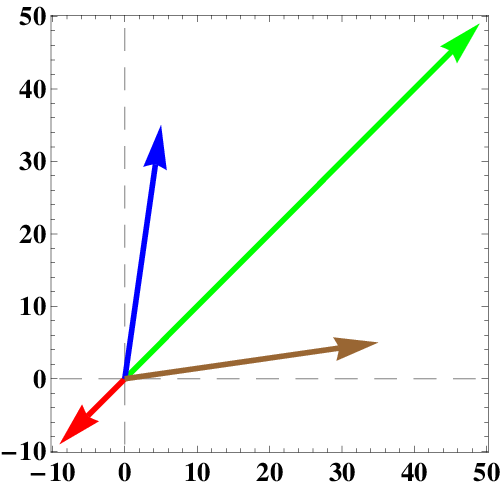
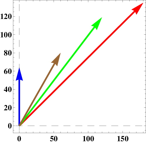
is a solution of (3), then each permutation of indexes or simultaneous and will generate a new solution of (6); in general case, all together 8 different symmetry generated solutions. Of course, in some particular cases, when some of the vectors belonging to a quartet coincide, the overall number of symmetry generated solutions can be smaller. For instance, the quartet is part of the cluster of 8 symmetry generated solutions, while the quartet belongs to the cluster of 4 such solutions. On the Fig. 1 the smallest tridents cluster is shown, with and without multi-edges. Graphical presentation of a cluster as a graph with multi-edges is of course mathematically correct but would make the pictures of bigger clusters somewhat nebulous (see Fig. 1, left panel). Notice that although formally we have solutions with multiplicities due to the symmetries, physically all these solutions correspond to the same quartet, and therefore we count them as one. Therefore, further on we omit multi-edges in our graphical presentations as it is shown in Fig. 1, right panel.


In the next sections, on all the Figures, the structure of resonance clusters in the spectral space is shown as follows: each wave vector is presented as a node of integer lattice and nodes belonging to one solution are connected by lines.
III Scale-resonances
We have studied the cluster structure of the scale-resonances in the spectral domain In our computational domain we have found 230464 such resonances, among them 213760 collinear (i.e. all 4 wave vectors are collinear) and only 16704 (7.25%) non-collinear resonances. However, the nonlinear interaction coefficient in collinear quartets is equal to zero and, therefore, they have no dynamical significance [24]. On the other hand, for mathematical completeness we will consider these solutions too, because there may exist 4-wave systems with the same dispersion law but with different forms of interaction coefficients such that are not necessarily zero on the collinear quartets.


In the Table I the structure of all clusters is presented while in the Table II - the structure of non-collinear is given; cluster length is the number of quartets belonging to one cluster.
| Cluster | Number of | Cluster | Number of |
|---|---|---|---|
| length | clusters | length | clusters |
| 1 | 43136 | 56 | 3 |
| 2 | 1256 | 60 | 6 |
| 8 | 452 | 72 | 1 |
| 10 | 184 | 80 | 1 |
| 12 | 20 | 92 | 2 |
| 16 | 14 | 128 | 1 |
| 20 | 10 | 152 | 1 |
| 40 | 7 | 176 | 1 |
| 48 | 2 | 208 | 1 |
| Cluster | Number of | Cluster | Number of |
|---|---|---|---|
| length | clusters | length | clusters |
| 1 | 1312 | 10 | 18 |
| 2 | 48 | 12 | 6 |
| 3 | 8 | 16 | 8 |
| 6 | 14 | 34 | 2 |
| 8 | 4 | 46 | 2 |
In Fig. 2 structure of collinear and non-collinear quartets is shown ia a smaller domain
III.1 Collinear quartets
First of all, let us make an important remark. If a 4-tuple consists of all collinear wave vectors, then the ratio is the same for all 4 wave vectors. Let us assume that , then
| (7) |
where is an arbitrary finite rational constant and
| (8) |
and Sys.(3) takes the form
Now we can compute taking arbitrary integer provided that is divisible on , and keeping in mind that , we can find all collinear solutions with Obviously, a rational number defines a line in the spectral space and not all the lines are allowed. Case corresponds to the solutions lying on the axes X () and Y (), i.e. with all or correspondingly, e.g. 4-tuple . Parametrization of the resonances in this case was first given in [24]. As we have already mentioned before, these quartets are dynamically irrelevant because there is no nonlinear interaction within these quartets [24].
III.2 Non-collinear quartets
III.2.1 Tridents
Non-collinear scale-resonances have been studied first in
[15, 9] in the spectral domain and a special type of quartets named tridents have
been
singled out. By definition, a wave quartet is called a trident if:
1) There exist two vectors among four in a quartet, say and ,
such that , thus they satisfy
;
2) Two other vectors in the quartet, and , have the same length: ;
3) and are equally inclined to
, thus
.
and two-parametric series of solutions has been written out:
| (10) |
with arbitrary integer . It is easy to check that vectors belong to the same class , with weights
and obviously
Parametrization (9) corresponds to the tridents oriented along the X-axis with its vectors and and, therefore, we will call them axial tridents. There exist also non-axial tridents, for instance, the quartet . As mentioned in [15, 9], all the non-axial tridents can be obtained from the axial ones, (9), via a rotation by angles with rational values of cosine combined with respective re-scaling (to obtain an integer-valued solution out of rational-valued ones).
| Cluster length | Number of clusters |
| 1 | 1320 |
| 2 | 48 |
| 6 | 40 |
| 12 | 10 |
| 18 | 2 |
| 22 | 2 |
In the computational domain , we have found 13888 non-axial tridents, the first non-axial trident is shown on the Fig. 3. Among 13888, 13504 tridents have no vectors on any axis and 384 tridents have just one vector on an axis (for instance, ). The total amount of all possible tridents is 14848, thus only 960 are axial ( of the total number). The data on tridents’ clustering are given in the Table III.
III.2.2 Non-tridents
Our study of the resonance solution set in the spectral domain shows that not all non-collinear cascading quartets are tridents. They are called further non-tridents, e.g. a quartet is a non-trident quartet.
The overall number of tridents is 14848 while the number of non-tridents is 1856. Notice that the first non-trident quartet lies in the spectral domain . This means, that if we are interested only in the large-scale quartets, say, quartets with the complete set of scale-resonances consists of 1728 quartets, among them - 1632 collinear quartets and 96 tridents, but no non-tridents yet.
III.3 Clusters
In the previous Section we have shown that there are three different types of scale-resonances: collinear quartets, tridents and non-tridents. There are also clusters formed by different types of scale-resonances, for instance, clusters containing tridents and non-tridents (Fig. 5, left panel) or collinear and non-collinear quartets (Fig. 5, right panel). Notice that, since collinear quartets of gravity water waves have zero interaction coefficients [24], the cluster shown on the right panel can dynamically be regarded as two independent quartets.

One of the most important characteristics of the resonance structure is the wavevector multiplicity (introduced in [20]), which describes how many times a given wavevector is a part of some solution. In the Table IV the wavevectors multiplicities are given for non-collinear quartets. It turned out that of all these wavevectors (6720 from overall amount 7384) have multiplicity 1 (counting the 8 symmetry generated solutions as the same quartet.)
| Multiplicity | Amount of vectors |
| 1 | 6720 |
| 2 | 424 |
| 3 | 192 |
| 4 | 36 |
| 5 | 8 |
| 6 | 4 |
In Fig. 1, we see an example of such a simple cluster consisting from just one physical quartet. In the Fig. 6 the cluster of 4 connected quartets is shown (the symmetry generated solutions are omitted), with all together only 7 different wave-frequencies.

Obviously, the cluster structure defines the form of dynamical system corresponding to the cluster. The main motivation of our detailed study of clusters is, of course, in constructing an isomorphism (i.e. one-to-one correspondence) between a cluster and a dynamical system. In [21] this construction has been presented for an arbitrary 3-wave resonance system, with triads as primary elements of the planar graph. Its implementation in Mathematica was given in [22], where interaction coefficients similar to in (18) were also computed. To construct this isomorphism two following facts were used: 1) in a 3-wave resonance system only scale-resonances exist, and 2) if we add an arbitrary triad to a cluster, in general we always add some new wave-frequencies as well (the only exception is identified in [21]). A 4-wave resonance system does not possess these nice properties; on the contrary - there exist scale- and angle-resonances, and most of the quartets are parts of symmetry generated solution sets. It would be a challenge to develop a general approach to construct dynamical systems for resonance clusters in an arbitrary 4-wave system.
IV Angle-resonances
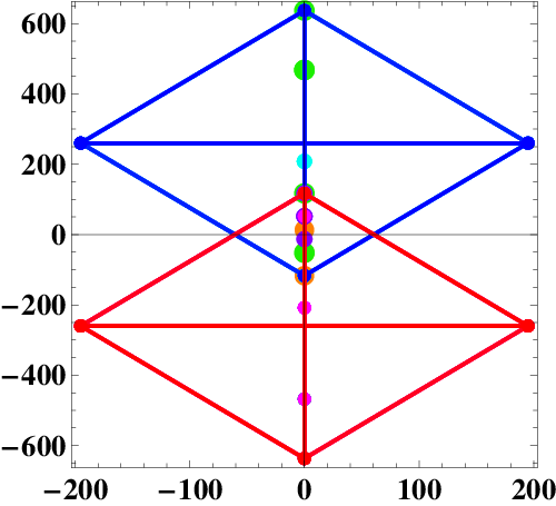
Until now we have studied the structure of the scale-resonances which are described by (4) and which generate new scales (i.e. new values of , thereby providing the energy cascade mechanism. The angle-resonances represented by (5) do not generate new scales but they can redistribute energy among the modes which were excited initially (or which are forced externally). Taken on their own, these resonances could lead to the thermal equilibrium distribution of the energy and the waveaction among the (initially excited) resonant waves, if the number of such waves is large, or they could lead to a periodical behavior or a strange attractor, if the number of the initially excited modes is small. The important fact, however, is that the scale- and the angle-resonances are not independent and can form a mixed cluster containing both types of this resonances [23]. The energy cascade mechanism in such a mixed cluster is presented schematically in Fig.7 where the quadrangles and denote scale-resonances so that 4-tuples and represent scale-resonances and squares represent angle-resonances.

If a wave takes part simultaneously in angle- and scale-resonances, corresponding nodes of and are connected by (red) dashed arrows so that and We have found many examples of such mixed clusters in our solution set, for instance:
with
which is further on connected with an angle-resonance
(not shown in Fig.7) via a node-vector .
The energy flux over scales due to the mixed cluster is weak: one wave can participate in a few dozen of angle-resonances (see Fig. 8), which means that only a small part of its energy will go to a scale-resonance. Moreover, even this weak energy cascade may terminate at finite wavenumber if it happens to move along a finite cluster which terminates before reaching the dissipation range (or before reaching the range of high frequencies where the nonlinearity gets large enough for the quasi-resonances to take over the energy flux from the exact resonances).

The number of angle-resonances in the spectral domain is of order of while the number of scale-resonances in the same domain is of order of , among them less than are non-collinear and do play a role in the energy exchange among the modes within the quartets (see next the Section). It is easy to see that an arbitrary wavevector takes part in infinite number of resonances if spectral domain is unbounded. Indeed, let us fix and then a quartet
| (11) |
a scale-resonance with arbitrary . More involved 5-parametric series of angle-resonances found from the following considerations. For angle-resonances of four wavevectors , Eqs.(3) can be rewritten as
| (12) |
Simple algebraic transformations and known parameterizations of the sum of two integer squares (e.g. for a circle or for the Pythagorean triples) yield
| (13) |
This is an easy task to check then that the solutions of (12) can be written out (perhaps with repetitions) via five integer parameters (rational solutions should be renormalized to integer). Notice that (11) degenerates to trivial resonances
| (14) |
if , i.e. it does not include any resonances of wavevectors of the form , for instance . In this case the choice in (13) gives
| (15) |
Analytical series are very helpful not only for computing resonance quartets and clusters structure but also while investigating the asymptotic behavior of interaction coefficients.

The multiplicity histogram for the angle-resonances is shown in Fig.9. On the axis the multiplicity of a vector is shown and on the axis the number of vectors with a given multiplicity. This graph has been cut off - multiplicities go very high, indeed the vector (1000,1000) takes part in 11075 solutions. All this indicates that the angle-resonances play an important role in the overall dynamics of the wave field.
V Dynamics
V.1 The wave field
Once the clusters are found, one can consider an evolution of amplitudes of waves that belong to each individual cluster by considering a respective reduction of the dynamical equation. For the gravity wave case, the appropriate dynamical equation is Zakharov equation for the complex amplitude corresponding to the -mode,
| (16) |
where is an interaction coefficient for gravity water waves which can be found in [25].
For very weak waves, amplitudes vary in time much slower than the linear oscillations. The factor on RHS will rapidly oscillate for most waves except for those in an exact resonance for which this factor is 1. Thus, only the resonant modes will give a contribution to the dynamics in this case and the oscillating contributions of the non-resonant terms will average out in time to zero and will not give any contribution to the cumulative change of . Leaving only the resonant terms, we have
| (17) |
where means a summation only over and which are in resonance with . Obviously, we should consider ’s from the same cluster only (i.e. solve the problem for one cluster at a time). Note that the fast timescale of the linear dynamics completely disappeared from this equation. Thus, paradoxically, the dynamics of very weak waves in finite boxes is strongly nonlinear: it is more nonlinear than in WTT which works for larger amplitudes and where quasi-resonances ensure phase randomness. This explains the fact found in the three-wave example that even relatively large clusters often exhibit a periodic or quasi-periodic behavior [26].
A study of the system (17) is possible analytically for small clusters (perhaps even integrating the system in some lucky cases) and numerically for large clusters, which is an interesting subject for future research. Some properties, however, can already be seen in the example of a single quartet which has been studied before [27]. Let us briefly discuss these properties.
V.2 A quartet
The dynamical system describing slowly changing amplitudes of a quartet has the form [27]:
| (18) |
and . The mathematical analysis of the system (18) can be performed similar to what has been done in [28] for an integrable 3-wave system of resonantly interacting planetary waves, though computations of the modulus of elliptic integral are more involved and variety of different dynamical scenarios is substantially reacher (see [27] for details). The general answer can be given in terms of Jacobean elliptic functions.
Obviously, the quartets with interaction coefficient do not influence the general dynamics of the wave field at the corresponding time scale. As it was shown in [24], for all collinear quartets , and therefore they can be excluded form consideration.
On the other hand, in [29] so-called ”degenerate quartets” (tridents in our terminology) have been studied and it was established numerically that they have strictly periodic behavior: after appropriate translation in the horizontal plane, two snapshots of the free-surface taken at and are identical.
For a general quartet and for arbitrary and arbitrary initial conditions, the system (18) ”does not exhibit strict periodicity” in numerical simulations [27]. Thus, the general formulae for the solutions of (18) have to be studied in more details in order to distinguish periodic and non-periodic dynamics of an arbitrary quartet. On the other hand, since our main interest in this paper is the large-scale dynamics, all scale-resonances with a non-zero interaction coefficient are tridents and therefore demonstrate a periodic time behavior. Of course, if a trident is involved into a cluster with some other quartets then one should be cautious about the predictions obtained for an isolated quartet.
VI Summary and Discussion of Results
• In this paper, we studied properties of deep water gravity waves bounded by a square periodic box. At very small wave amplitudes, when the nonlinear resonance broadening is less than the -space spacing, WTT fails and only the waves which are in exact four-wave resonance can interact. This situations appears to be typical for all existing numerical simulations [9] and laboratory experiments [10]. Thus, to understand the wave behavior in laboratory experiments and in numerical simulations it is crucial to study exact resonances among discrete wave modes, which was the focus of the present paper. Of course, the notation of ”very small amplitudes” has to be worked out explicitly for interpreting the results of laboratory experiments. The smallness of amplitudes is defined by the choice of a small parameter and depends of the intrinsic characteristics of the wave system, for instance, for atmospheric planetary waves it is usually taken as the ratio of the particle velocity to the phase velocity which allows to obtain explicit estimation [30] for a wave amplitude (corresponding to the weakly nonlinear regime) as a function of and . For the water surface waves, the wave steepness, , is usually taken as a small parameter and corresponds then to the weakly nonlinear regime. For such weakly nonlinear waves to feel discreteness of the -space, their nonlinear frequency broadening has to be less than the distance between adjacent -modes. In terms of the wave steepness this condition reads , see [15, 9].
• We found numerically all resonant quartets on the set of 1000 x 1000 modes making use of the -class method originally developed in [18]. We found that all resonant quartets separate into noninteracting with each other clusters. Each cluster may consist of two types of quartets: scale- and angle-resonances. The angle-resonances cannot transfer energy to any -modes which are not already present in the system. They cannot carry an energy flux through scales and their main role is to thermalize the initially excited modes. The scale-resonances are much more rare than the angle ones and yet their role is important because they are the only resonances that can transfer energy between different scales. Most of the scale-resonances, but not all, are of the trident type, for which a partial parametrization can be written out explicitly. If one is interested in large-scale modes only, say 100 x 100 domain, then the tridents are the only scale-resonances, which is very fortunate due to the available parametrization.
• Even though the angle-resonances cannot cascade energy, they are important for the overall cascade process because they are involved in the same wave clusters with the scale-resonances. One wave mode may typically participate in many angle resonances and only one scale resonance. Thus, one can split large clusters into ”reservoirs”, each formed by a large number of angle quartets in quasi-thermal equilibrium, and which are connected with each other by sparse links formed by scale quartets. This structure suggests a significant energy cascade slowdown and anisotropy with respect to the infinite-box limit. Further study is needed to examine the structure of such large clusters and possible energy cascade routes from the region of excitation at low wavenumbers to the dissipative large range. In the essentially finite domain the situation is opposite. Quite recently results of the laboratory experiments with surface waves on deep water were reported [31, 32, 33] in which regular, nearly permanent patterns of the water surface have been observed. A feasible way to interpret these results would be 1) to establish that the conditions of the experiments correspond to the weakly nonlinear regime; if yes - to proceed as follows: 2) to compute all exact resonances in the wave-lengths range corresponding to those in the experiments; 3) to demonstrate that for chosen wave-lengths and the size of laboratory tank no scale-resonances appear, 4) to attribute the regular patterns to the corresponding angle-resonances. Obviously, the scale-resonances would produce the spectrum anisotropy and disturb the regular patterns.
• We also discussed consequences of the cluster structures for the dynamics, and argued that one should expect a less random and more regular behavior in the case of very low amplitude waves with respect to larger (but still weak) waves described by WTT. More study is needed in future both analytically, for small clusters, and numerically, for large clusters. A particularly interesting question to answer in this case is about any possible universal mechanisms of transition between the regular dynamics to chaos and possible coexistence of the regular and chaotic motions.
• Last not least. The knowledge of the 2D-resonance structure might yield new insights into the origin of some well-known physical phenomena, for instance, Benjamin-Feir (B-F)instability [34] or McLean instability. This is ”a modulational instability in which a uniform train of oscillatory waves of finite amplitude losses energy to a small perturbation of waves with nearly the same frequency and direction” [35]. As it was shown recently in [36, 37, 35], the modulational instability, though well established not only water waves theory but also in plasmas and optics, has to be seriously reconsidered. It turned out that 1) it can be shown analytically that arbitrary small dissipation stabilizes the B-F instability, and 2) results of laboratory experiments show that B-F theory generally over-predicts the growth rate. Moreover, the growth rate changes with the time [35]. Some researchers state even that ”… this effect is far less significant than was believed and should be disregarded” [38]. The other way to treat the problem would be to try and and explain the modulational instability through non-collinear (that is, essentially two-dimensional) exact resonances [39]. Similar questions arise in the study of McLean instabilities defined by the magnitudes of the water depth on which surface waves are studied. For instance, as it was demonstrated in [40], in some regimes of shallow water the instabilities are due to higher order resonances among 5 to 8 waves. It would, therefore, be interesting to see how the B-F and McLean instabilities are modified by the finite flume effects and the corresponding discreteness of the wave resonances, and to see what role this could have played in the past laboratory and numerical experiments. Results presented in our paper can be regarded as a necessary first step for such an investigation, and the future work would involve application of the -class method to computing the higher order resonances which may be involved in modulational instabilities.
Acknowledgments
Acknowledgements. E.K. acknowledges the support of the Austrian Science Foundation (FWF) under project P20164-N18 ”Discrete resonances in nonlinear wave systems”. O.R. and S.N. acknowledge the support of the Transnational Access Programme at RISC-Linz, funded by European Commission Framework 6 Programme for Integrated Infrastructures Initiatives under the project SCIEnce (Contract No. 026133). Authors are genuinely grateful to both anonymous Referees whose suggestions made the form our paper more clear and led, in particularly, to including the very important paragraph about Benjamin-Fair and McLean instabilities. Authors express a special gratitude to Victor L’vov for fruitful and stimulating discussions.
References
- [1] V.E. Zakharov, V.S. L’vov and G. Falkovich. Kolmogorov Spectra of Turbulence. Series in Nonlinear Dynamics, Springer (1992)
- [2] Y. Lvov and S.V. Nazarenko, Phys. Rev. E: 69: 066608 (2004)
- [3] Y. Choi, Y. Lvov, S.V. Nazarenko and B.Pokorni. Physics Letters A: 339 (3-5): 361 (2004)
- [4] Y. Choi, Y. Lvov and S.V. Nazarenko. Physics Letters A: 332 (3-4): 230 (2004)
- [5] A.C. Newell, S.V. Nazarenko and L. Biven, Physica D 152-153: 520 (2001)
- [6] A.N. Pushkarev and V.E. Zakharov, Physica D 135 (1-2): 98 (2000)
- [7] V.E. Zakharov, A.O. Korotkevich, A.N. Pushkarev and A.I. Dyachenko, JETP Lett. 82 (8): 487 (2005)
- [8] S. Annenkov and V. Shrira, Phys. Rev. Lett 96: 204501 (2006)
- [9] Y.V. Lvov, S. Nazarenko and B. Pokorni. Physica D 218: 24 (2006)
- [10] P. Denissenko, S. Lukaschuk and S. Nazarenko, Phys. Rev. Lett. 99: 014501 (2007)
- [11] E. Falcon, C. Laroche and S. Fauve. Phys. Rev. Lett. 98: 094503 (2007)
- [12] G. Kolmakov, A. Levchenko, M. Braznikov, L. Mezhov-Deglin, A. Slichenko and P. McClintock. Phys. Rev. Lett. 93: 74501 (2004)
- [13] M. Braznikov, G. Kolmakov, A. Levchenko and L. Mezhov-Deglin. Europhysics Lett. 58: 510 (2002)
- [14] V. M. Eguíluz, M. T. Levinsen and P. Alstrom. Europhys. Lett. 58: 517 (2002)
- [15] S. Nazarenko. J. Stat. Mech. LO2002 (2006)
- [16] E. Kartashova. Phys. Rev. Lett. 72: 2013 (1994)
- [17] E. Kartashova. AMS Transl. 182 (2): 95 (1998)
- [18] E. Kartashova. J. Low Temp. Phys. 145 (1-4): 286 (2006)
- [19] E. Kartashova and A. Kartashov. Int. J. Mod. Phys. C 17(11): 1579 (2006)
- [20] E. Kartashova and A. Kartashov. Comm. Comp. Phys. 2 (4): 783 (2007)
- [21] E. Kartashova and G. Mayrhofer. Physica A: Stat. Mech. Appl. 385: 527 (2007)
- [22] E. Kartashova, C. Raab, Ch. Feurer, G. Mayrhofer and W. Schreiner. In Ch. Kharif, E. Pelinovsky (Eds): Extreme Waves in the Ocean, Springer (to appear). E-print: http://arxiv.org/abs/0706.3789) (2008)
- [23] E. Kartashova. Phys. Rev. Lett. 98 (21): 214502 (2007)
- [24] A.I. Dyachenko, Y.V. Lvov and V.E. Zakharov, Physica D 87 (1-4): 233 (1995)
- [25] V.P. Krasitskii. J. Fluid Mech. 272: 1 (1994)
- [26] E. Kartashova and V.S. L’vov. Submitted to Phys. Rev. Lett. E-print arXiv:0801.3374v1 (2008)
- [27] M. Stiassnie and L. Shemer. Wave motion 41: 307 (2005)
- [28] E. Kartashova and V.S. L’vov. Phys. Rev. Lett. 98 (19): 198501 (2007)
- [29] L. Shemer and M. Stiassnie. In Y. Toba, H. Mitsuyasu, F.D. Reidel (Eds): The ocean surface, p.51-57. Dodrecht, Holland (1985)
- [30] E.A. Kartashova. Theor. Math. Phys. 99: 1510 (1994)
- [31] H. Segur and D.M. Henderson. Euro. Phys. J. – Special Topics 147: 25 (2007)
- [32] W. Craig, D.M. Henderson, M. Oscamou and H. Segur. Math. Comput. Simul, doi: 10.1016/ j.matcom. (2006)
- [33] D.M. Henderson, M.S. Patterson and H. Segur. (2006) J. Fluid Mech. 559: 413 (2006)
- [34] T.B. Benjamin and J.E. Feir. J. Fluid Mech. 27: 417 (1967)
- [35] H. Segur, D. Henderson, J. Hammack, C.-M. Li, D. Pheiff. and K. Socha. J. Fluid Mechanics 539: 229 (2005)
- [36] J.L. Hammack, D.M. Henderson. J. Offshore Mech. Artic Eng. 125: 48 (2003)
- [37] J.L. Hammack, D.M. Henderson and H. Segur. J. Fluid Mechanics 532: 1 (2005)
- [38] B.M. Lake and H.C. Yuen. J. Fluid Mech. 83: 75 (1977)
- [39] This idea has been discussed by one of the authors, E.K., and late Joe Hammack in 1995. But at that time -class method was not yet implemented, exact resonances could not be computed and all the reasoning was rather theoretical.
- [40] M. Francius and C. Kharif. Geophysical Research Abstracts 7: 08757 (2005)