Efficient simulation of quantum evolution using dynamical coarse-graining.

The number of independent observables of a quantum system with the Hilbert space dimension $N$ is $N^{2}-1$. In many-body systems, when $N$ increases exponentially with the number of degrees of freedom, that large number of observables can be neither measured nor calculated. Only a limited number of dynamical variables is accessible to an experimentalist, while all the uncontrollable parameters are averaged out. This means that generically, an observed quantum system is characterized by a small number of the expectation values of accessible observables. To theoretically characterize the dynamics of a quantum system it is desirable: (i) to find equations of motion for this reduced set of expectation values; (ii) to be able to solve the associated equations of motion efficiently. A computational cost of a direct quantum simulation scales as $O(N^{\delta})$, $\delta>1$ [1]. A simulation is defined as efficient if the corresponding equations of motion can be solved with a computational cost which is reduced substantially from that number.

In the present study we explore the possibility of an efficient simulation of a restricted set of observables, using a novel paradigm for the simulation. Assuming that the set of experimentally accessible observables is small, it is plausible that there exist a number of microscopic theories, leading to the same observed dynamics. If a microscopic theory can be found, which leads to equations of motion that can be solved efficiently, the dynamics of the restricted set of observables can be efficiently simulated. More specifically, we propose to simulate the unitary dynamics of a quantum system by embedding it in a particular open system dynamics. In this dynamics the coupling to the bath is constructed to have a negligible impact on the evolution of the selected set of observables on the characteristic time scale of their unitary evolution. The key point is that the resulting open system dynamics can be efficiently simulated. The reduction of the computational complexity of the evolution, imposed by the bath, is attributed to dynamical coarse-graining, collapsing the system to a preselected representation which is used as the basis for the dynamical description. Since the bath has no observable effect by construction it should be considered solely as a computational tool. For that reason a term fictitious bath is used in the paper to refer to it.

The quantum systems considered in the present work have finite Hilbert space dimension. The dynamics is generated by the Lie-algebraic Hamiltonians:

$\displaystyle{{\mathrm{\hat{H}}}}=\sum_{i}a_{i}{{\mathrm{\hat{X}}}}_{i}+\sum_{ij}b_{ij}{{\mathrm{\hat{X}}}}_{i}{{\mathrm{\hat{X}}}}_{j},$

(1)

where the set $\{{{\mathrm{\hat{X}}}}_{i}\}$ of observables is closed under the commutation relations:

$\displaystyle\left[{{\mathrm{\hat{X}}}}_{i},{{\mathrm{\hat{X}}}}_{j}\right]=i\sum_{k=1}^{K}f_{ijk}{{\mathrm{\hat{X}}}}_{k},$

(2)

i.e., it forms the spectrum-generating [2] Lie algebra [3] of the system. This algebra is labeled by the letter $\mathfrak{g}$ in what follows. Lie-algebraic Hamiltonians (1) are abundant in molecular [4, 5], nuclear [2, 5] and condensed matter physics [2] . The basis of the algebra $\{{{\mathrm{\hat{X}}}}_{i}\}$ is chosen as a distinguished set of observables, which are to be simulated efficiently. Lie algebras considered in the present work are compact semisimple algebras [3] and the basis $\{{{\mathrm{\hat{X}}}}_{i}\}$ is assumed to be orthonormal with respect to the Killing form [3].

The corresponding open system dynamics, which is alleged to simulate the unitary dynamics of the elements of $\mathfrak{g}$, is governed by the following Liouville-von Neumann equation of motion

$\displaystyle\frac{\partial}{\partial t}{{\mathrm{\hat{\rho}}}}={\cal L}{{\mathrm{\hat{\rho}}}}=-i\left[{{\mathrm{\hat{H}}}},{{\mathrm{\hat{\rho}}}}\right]-\gamma\sum_{j=1}^{K}\left[{{\mathrm{\hat{X}}}}_{j},\left[{{\mathrm{\hat{X}}}}_{j},{{\mathrm{\hat{\rho}}}}\right]\right],$

(3)

which has the Lindblad form [6, 7], i.e., it describes a Markovian completely positive [7] nonunitary evolution of the quantum system. The physical interpretation of the evolution, governed by Eq.(3) is the process of weak measurements [8] of the algebra of observables $\mathfrak{g}$, performed on the quantum system, evolving under the Hamiltonian (1).

The foundation of the method is the observation that coupling to the bath induces a decoherence of the evolving density operator in a particular basis known as generalized coherent states (GCS), associated with the algebra (Section II). It is shown that if the Hamiltonian is linear in ${{\mathrm{\hat{X}}}}_{i}$ and a certain ”classicality condition” is satisfied by the Hilbert space representation of the algebra, the decoherence time-scale is much shorter than the timescale on which the effect of the bath on the elements of $\mathfrak{g}$ is measurable, i.e., the relaxation time-scale. It is conjectured that this strong time separation will also hold for Hamiltonians bilinear in the elements of $\mathfrak{g}$ (Section III).

We propose to take advantage of this property of the open system dynamics for efficient simulation of the unitary evolution of $\{{{\mathrm{\hat{X}}}}_{i}\}$, using stochastic unravelings of the evolution [9, 10, 11] and representing the evolving stochastic pure state in the time-depending basis of the GCS [12, 13] (Section IV). The effect of the decoherence translates into localization of evolving stochastic pure state in the GCS basis, which enables efficient representation and simulation of the stochastic evolution. Averaging over the unravelings recovers the unitary dynamics of the algebra generators. It is shown that the averaging can be performed efficiently provided the corresponding dynamics can be efficiently measured in the lab. The effect of coupling to the fictitious bath is illustrated by the dynamics of a Bose-Einstein condensate (BEC) in a double-well trap [14, 15] modeled by the two-mode Bose-Hubbard Hamiltonian (Section V). It is demonstrated that the bath induces drastic localization on the level of a stochastic pure-state evolution, while having no observed effect on the dynamics of the elements of the spectrum-generating algebra of the system.

A central theme in this section is the intimate relation between the evolution of the subalgebra of observables and the dynamics of the generalized coherent states (GCS) associated with this subalgebra. The GCS minimize the total uncertainty with respect to the basis elements of the subalgebra and in addition are maximally robust to interaction with the bath, modeled by Eq.(3).

The purpose of the present section is to show that the classicality condition (13) implies a large time-scales separation between the decoherence of the state and the relaxation of the observables comprising the spectrum-generating algebra of the system, if the Hamiltonian (1) is linear in the generators of the algebra. It is conjectured that the time-scales separation is preserved by the Hamiltonians at most bilinear in the generators. As a consequence, the unitary evolution of the observables on the intermediate time scale can be simulated by the open system dynamics, while the effect of the decoherence can be employed for efficient simulation of the open dynamics.

Consider an Hamiltonian linear in the elements of the algebra $\mathfrak{g}$, i.e., all $b_{ij}=0$ in Eq. (1). The corresponding Heisenberg equations for the observables in $\mathfrak{g}$ becomes:

	$\displaystyle\frac{\partial}{\partial t}{{\mathrm{\hat{X}}}}_{i}$	$\displaystyle=$	$\displaystyle-i\left[{{\mathrm{\hat{H}}}},{{\mathrm{\hat{X}}}}_{i}\right]-\gamma\sum_{j=1}^{K}\left[{{\mathrm{\hat{X}}}}_{j},\left[{{\mathrm{\hat{X}}}}_{j},{{\mathrm{\hat{X}}}}_{i}\right]\right]$		(14)
		$\displaystyle=$	$\displaystyle-i\sum_{k=1}^{K}\left(ia_{ik}\right){{\mathrm{\hat{X}}}}_{k}-\gamma\sum_{j,l=1}^{K}\left(if_{jik}\right)\left(if_{jkl}\right){{\mathrm{\hat{X}}}}_{l}$
		$\displaystyle=$	$\displaystyle-i\sum_{k=1}^{K}\left(ia_{ik}\right){{\mathrm{\hat{X}}}}_{k}-\gamma\sum_{j,l=1}^{K}\left(T^{j}\right)^{2}_{il}{{\mathrm{\hat{X}}}}_{l},$

where $T^{i}_{jk}=if_{ijk}$ is a matrix element of the adjoint representation [3] of ${{\mathrm{\hat{X}}}}_{i}$. It is assumed without loss of generality that $\mathfrak{g}$ is a compact simple subalgebra of observables ( in the general case of a semisimple algebra, the system of Eqs.(14) decouples into systems of equations for the simple components of the algebra). The coefficients in the r.h.s. of (14) obey

$\displaystyle\sum_{j=1}^{K}\left(T^{j}\right)^{2}=C_{2}$

(15)

where $C_{2}$ is the quadratic Casimir of $\mathfrak{g}$ in the adjoint representation. Therefore

$\displaystyle\left(\sum_{j=1}^{K}\left(T^{j}\right)^{2}\right)_{il}=(C_{2})_{il}=c_{\texttt{adj}}\delta_{il}$

(16)

leading to

$\displaystyle\frac{\partial}{\partial t}{{\mathrm{\hat{X}}}}_{i}$

$\displaystyle=$

$\displaystyle-i\sum_{k=1}^{K}\left(ia_{ik}\right){{\mathrm{\hat{X}}}}_{k}-\gamma c_{\texttt{adj}}{{\mathrm{\hat{X}}}}_{i},$

(17)

which in a matrix notation reads

$\displaystyle\frac{\partial}{\partial t}{{\mathrm{\hat{X}}}}$

$\displaystyle=$

$\displaystyle-i\left(A-\gamma c_{\texttt{adj}}\right){{\mathrm{\hat{X}}}},$

(18)

where $A=A^{\dagger}$ is defined by $A_{kl}=ia_{kl}$ and ${{\mathrm{\hat{X}}}}\equiv\{{{\mathrm{\hat{X}}}}_{1},{{\mathrm{\hat{X}}}}_{2},...{{\mathrm{\hat{X}}}}_{k}\}$. We define ${{\mathrm{\hat{Y}}}}\equiv\{{{\mathrm{\hat{Y}}}}_{1},{{\mathrm{\hat{Y}}}}_{2},...{{\mathrm{\hat{Y}}}}_{k}\}$ by

$\displaystyle\frac{\partial}{\partial t}{{\mathrm{\hat{Y}}}}_{i}$

$\displaystyle=$

$\displaystyle-iA{{\mathrm{\hat{Y}}}}_{i}=-i\omega_{i}{{\mathrm{\hat{Y}}}}_{i},$

(19)

where $\omega_{i}$ are real since $A$ is Hermitian. Then ${{\mathrm{\hat{Y}}}}$ diagonalize also Eq.(18):

$\displaystyle\frac{\partial}{\partial t}{{\mathrm{\hat{Y}}}}_{i}$

$\displaystyle=$

$\displaystyle\left(-iA-\gamma c_{{\texttt{adj}}}\right){{\mathrm{\hat{Y}}}}_{i}=\left(-i\omega_{i}-\gamma c_{\texttt{adj}}\right){{\mathrm{\hat{Y}}}}_{i},$

(20)

leading to the solution of Eq.(18):

$\displaystyle{{\mathrm{\hat{Y}}}}_{i}(t)$

$\displaystyle=$

$\displaystyle{{\mathrm{\hat{Y}}}}_{i}(0)e^{-\left(i\omega_{i}+\gamma c_{\texttt{adj}}\right)t}$

(21)

and

$\displaystyle{{\mathrm{\hat{X}}}}_{i}(t)=\sum_{j}c_{ij}{{\mathrm{\hat{Y}}}}_{i}(t).$

(22)

The solution (21) is obtained for an arbitrary compact simple subalgebra of the system observables $\mathfrak{g}\cong\mathfrak{su}(K)\subseteq\mathfrak{su}(N)$ for a quantum system in a $N$-dimensional Hilbert space. It can be generalized to a semisimple subalgebra of observables, i.e., a direct sum of simple subalgebras, $\mathfrak{g}=\oplus_{i=1}^{n}\mathfrak{su}(K_{i})\subseteq\mathfrak{su}(N)$, corresponding to a tensor-product partition of the system Hilbert space ${\cal H}=\otimes_{i=1}^{n}{\cal H}_{i}$. In this case, Eq.(21) corresponds to local observables of any given subsystem.

From Eq.(21) we see that the expectation values of observables in $\mathfrak{g}$ oscillate on the timescales $\omega_{i}$ and decay on the time scale $\gamma c_{\texttt{adj}}$. Consider an observable ${{\mathrm{\hat{Y}}}}_{i}$ such that $\omega_{i}\gg\gamma c_{\texttt{adj}}$. When the measurement of ${{\mathrm{\hat{Y}}}}_{i}$ in a time interval

$\displaystyle(\omega_{i})^{-1}\ll\tau\ll(\gamma c_{\texttt{adj}})^{-1},$

(23)

is performed, the nonunitary character of the evolution cannot be discovered. Therefore, given the time interval $\tau$ any $\gamma$ with the property $\tau\ll(\gamma c_{\texttt{adj}})^{-1}$ will lead to apparently unitary dynamics of ${{\mathrm{\hat{Y}}}}_{i}$ on the time interval $\tau$ .

Next we note that since $(\Lambda,\mu)\neq 0$ in Eq.(11) (a positive root has strictly positive scalar product with the maximal weight vector) strong inequality (13) implies $|\Lambda|\gg|\mu|$, which leads to the following strong inequality

$\displaystyle\sqrt{c_{\cal H}}\gg\sqrt{c_{\texttt{adj}}}.$

(24)

Therefore, a time interval $\tau$ exists such that

$\displaystyle(\gamma c_{\cal H})^{-1}\ll\omega_{i}^{-1}\ll\tau\ll(\gamma c_{\texttt{adj}})^{-1}.$

(25)

for some $i$ corresponding to an observable ${{\mathrm{\hat{Y}}}}_{i}$ in Eq.(21). The lhs of the inequality (25) is the decoherence rate of a generic superposition of the GCS with respect to the algebra $\mathfrak{g}$ and the lhs is the decay rate of the observable ${{\mathrm{\hat{Y}}}}_{i}$. This system of strong inequalities implies two important properties of the open system dynamics, Eqs.(14): (i) a generic superposition of the GCS collapses into a mixture of the GCS on a time scale much shorter than a physically interesting time scale of the unitary evolution of the observable; (ii) the time scale of the unitary evolution of the observable is much shorter than its relaxation time scale.

It should be to emphasized that the classicality condition (13) is not sufficient to imply properties (i) and (ii) in a generic case of nonlinear Hamiltonians (1). Generic nonlinearity in the Hamiltonian is expected to introduce faster time-scales in the relaxation of the observables. The crucial question is whether these timescales are as short as the decoherence timescale $(\gamma c_{\cal H})^{-1}$. Since the decoherence time-scale depends not only on the algebra but also on its Hilbert space representation, it seems that in order to introduce as fast time-scales into the relaxation, the nonlinearity should effectively couple most of the Hilbert-Schmidt basis of the system operators on the physically interesting time-scale of the unitary evolution of the algebra elements. It is conjectured that a Hamiltonians at most bilinear in the elements of the spectrum-generating algebra does not possess such strong coupling property. A closer investigation of this important question is left to future research.

Efficient simulation is defined as a simulation based on a numerical solution of the first order differential equations for a number of dynamical variables which is much smaller than the Hilbert space dimension of the system. The number of dynamical variables $m$ cannot be smaller than the number of observables to be simulated, which equals the dimension $K$ of the spectrum-generating algebra $\mathfrak{g}$. If there is a large gap between the dimension of the algebra and the Hilbert space dimension $K=\texttt{dim}\{\mathfrak{g}\}\ll\texttt{dim}\{{\cal H}\}=N$ the simulation based on the the number of variables $K\lesssim m\ll N$ is considered efficient.

The principle of efficient simulation of the observables, forming the spectrum-generating algebra $\mathfrak{g}$ of the Hamiltonian (1) is based upon

• •

  Simulating the unitary evolution of the observables by the fictitious open system dynamics, governed by the Liouville-von Neumann Eq.(3);

• •

  Unraveling the Liouville-von Neumann Eq.(3) into pure state evolutions, governed by the stochastic nonlinear Schrödinger equation (sNLSE) (see below);

• •

  Efficient simulation of the stochastic nonlinear pure state dynamics, using expansion of the state in a time-dependent basis of the generalized coherent states (GCS), associated with the spectrum-generating algebra $\mathfrak{g}$.

In the previous section we have discussed the first of the listed items. The other two items focus on the principles of efficient simulation of the open-system evolution.

Solving directly the Liouville-von Neumann master Eq.(3) is more difficult than the original problem. A reduction in complexity is based on the equivalence between the Liouville-von Neumann equation and the stochastic nonlinear Schrödinger equation (sNLSE)[9, 10, 11]:

$\displaystyle d\left|{\psi}\right\rangle$

$\displaystyle=$

$\displaystyle\left\{-i{{\mathrm{\hat{H}}}}dt-\gamma\sum_{i=1}^{K}\left({{\mathrm{\hat{X}}}}_{i}-\left\langle{{\mathrm{\hat{X}}}}_{i}\right\rangle_{\psi}\right)^{2}dt+\sum_{i=1}^{K}\left({{\mathrm{\hat{X}}}}_{i}-\left\langle{{\mathrm{\hat{X}}}}_{i}\right\rangle_{\psi}\right)d\xi_{i}\right\}\left|{\psi}\right\rangle,$

(26)

where the Wiener fluctuation terms $d\xi_{i}$ satisfy

$\displaystyle<d\xi_{i}>=0,\ \ \ d\xi_{i}d\xi_{j}=2\gamma dt.$

(27)

To demonstrate the equivalence, Eq.(26) can be cast into the evolution of the projector ${{\mathrm{\hat{P}}}}_{\psi}=\left|\psi\right\rangle\left\langle\psi\right|$

$\displaystyle d{{\mathrm{\hat{P}}}}_{\psi}=\left(-i\left[{{\mathrm{\hat{H}}}},{{\mathrm{\hat{P}}}}_{\psi}\right]-\gamma\sum_{j=1}^{K}\left[{{\mathrm{\hat{X}}}}_{j},\left[{{\mathrm{\hat{X}}}}_{j},{{\mathrm{\hat{P}}}}_{\psi}\right]\right]\right)dt+\sum_{i}\left\{\left({{\mathrm{\hat{X}}}}_{i}-\left\langle{{\mathrm{\hat{X}}}}_{i}\right\rangle_{\psi}\right)d\xi_{i},{{\mathrm{\hat{P}}}}_{\psi}\right\}.$

(28)

Averaging Eq.(28) over the noise recoveres the original Liouville-von Neumann equation (3). Therefore, the problem of efficient simulation of the Liouville-von Neumann dynamics is transformed to the problem of efficient simulation of the nonlinear stochastic dynamics, governed by sNLSE Eq. (26).

The simulation of the pure state evolution according to the sNLSE(26) is based on an expansion of the evolving state in the time-dependent basis of the GCS, Eq.(4). In the case of a finite Hilbert space an arbitrary state can be represented as a superposition of $M\leq N$ GCS:

$\displaystyle\left|\psi\right\rangle=\sum_{i=1}^{M}c_{i}\left|\Omega_{i},\Lambda\right\rangle,$

(29)

where $\Omega_{i}$ is an element of the coset space $G/H$, $G$ is the dynamical group of the system generated by $\mathfrak{g}$, $H$ is the maximal stability subgroup, corresponding to the reference state $\left|\Lambda\right\rangle$ and $\Lambda$ is the highest weight of the Hilbert space representation of the algebra. The coset space $G/H$ has natural symplectic structure [13] and can be considered as a phase space of the quantum system, corresponding to $\mathfrak{g}$. Accordingly, $\Omega_{i}$ is a point in the phase space. The total number of variables defining (up to an overall phase) the state $\psi$ (29) equals $M$ times the dimension of the phase space $G/H$ plus the number $M$ of amplitudes $c_{i}$. The dimension of $G/H$ depends on the properties of the Hilbert space representation of the algebra, but is always strictly less then the dimension of the algebra $K$ [13]. Therefore, the number $m$ of real parameters, characterizing the state $\psi$ (29) satisfies the following inequality

$\displaystyle m<M(K+2).$

(30)

It follows that the necessary condition for efficient simulation of the dynamics is that $1\lesssim M\ll N$ in the physically relevant time interval.

It is assumed that initial state of the system is a GCS, corresponding to $M=1$ in the expansion (29). If one omits the nonlinear and stochastic terms in the Eq.(26) it becomes a regular Schröedinger equation, governing the unitary evolution of the state. If the Hamiltonian in Eq.(26) is linear in the elements of $\mathfrak{g}$, the initial GCS evolves into a GCS by the definition, Eq.(6). Restoring the nonlinear and stochastic terms to Eq.(26) breaks the unitarity of the evolution but a GCS still evolves into a GCS under the full equation, Ref.[20]. Therefore a GCS solves the sNLSE(26), driven by a linear Hamiltonian. In Ref.[20] it is proved that a CGS is a globally stable solution in that case, i.e., an arbitrary initial state evolves asymptotically into a GCS.

Adding bilinear terms to the Hamiltonian (1) breaks the invariance of the subalgebra $\mathfrak{g}$ under the action of the Hamiltonian and, as a consequence, an initial GCS evolves into a superposition of a number $M>1$ of the GCS (29) in the corresponding unitary evolution. If the number of terms $M$ becomes large, $M=O(N)$, the unitary evolution can no longer be simulated efficiently. The nonlinear and stochastic terms (representing the effect of the fictitious bath) in Eq.(26) is expected to decrease the effective number $M$ of terms in the expansion (29) of the evolving state. This effect will be termed localization. The natural measure of the localization is the total uncertainty of the evolving state with respect the spectrum-generating algebra $\mathfrak{g}$ or, equivalently, the generalized purity of the state with respect to $\mathfrak{g}$ [21].

The localizing effect of the bath is proved in the Ref.[20]. Heuristically, it can be understood as follows. If each sum in the sNLSE (26) is replaced by a single contribution of a given operator ${{\mathrm{\hat{X}}}}$ the uncertainty of the evolving state with respect to ${{\mathrm{\hat{X}}}}$ is strictly decreasing under the action of the bath, unless the state is an eigenstate of ${{\mathrm{\hat{X}}}}$, in which case it vanishes [9, 10, 11]. Therefore, the effect of the bath is to bring an arbitrary state into an eigenstate of ${{\mathrm{\hat{X}}}}$. In our case, the observables ${{\mathrm{\hat{X}}}}_{i}$ are noncommuting and cannot be diagonalized simultaneously. Therefore, it is expected that the effect of the bath in this case will be to take an arbitrary state to the state which minimizes the total uncertainty with respect to the elements of the algebra, i.e., to a GCS.

The characteristic time scale of the localization is the decoherence time scale $(\gamma c_{\cal H})^{-1}$. If the classicality condition (13) holds and the nonlinearity of the Hamiltonian is moderate (Cf. the end of Section III), the localization is effective on a time interval much shorter than the relaxation of the observables in $\mathfrak{g}$. As a consequence, the unitary dynamics of these observables can be obtained by (i) simulating the nonlinear stochastic evolution of the localized pure states, (ii) calculating the expectation values of the observables in each stochastic unraveling and (iii) averaging over the stochastic realizations.

Calculating the expectation values and averaging (steps (ii) and (iii) above) are not part of the definition of efficient simulation, and therefore should be considered separately. Even if the step (i) can be performed efficiently according to the definition, it is left to show that the complexity of performing steps (ii) and (iii), measured, for example, by a number of elementary computer operations, scale substantially less than the size of the Hilbert space dimension.

To calculate the expectation value of an observable in a state represented by the GCS expansion (29) one has to calculate $M(M+1)/2$ matrix elements of the operator between the GCS. Each matrix element for an operator ${{\mathrm{\hat{X}}}}_{i}\in\mathfrak{g}$ can be calculated group-theoretically [13, 22], i.e., independently on the Hilbert space representation. Therefore, if $M\ll N$ the computation of the expectation values of the elements of $\mathfrak{g}$ can be performed efficiently.

Complexity of the step (iii) is measured by the number of stochastic realizations necessary to obtain the expectation values of the observables to a prescribed accuracy. In Appendix C it is shown that the averaging can be performed efficiently, provided the expectation values of the elements of $\mathfrak{g}$ can be measured efficiently. More precisely

$\displaystyle n_{st}(\epsilon)\leq n_{ex}(\epsilon)\texttt{dim}\{\mathfrak{g}\},$

(31)

where $n_{st}(\epsilon)$ is the number of stochastic realizations, necessary to obtain the expectation value of each observable ${{\mathrm{\hat{X}}}}_{i}\in\mathfrak{g}$ to an absolute accuracy $\epsilon$, $n_{ex}(\epsilon)$ is the number of experimental runs, necessary to obtain the expectation value of each ${{\mathrm{\hat{X}}}}_{i}$ to the absolute accuracy $\epsilon$ and $\texttt{dim}\{\mathfrak{g}\}$ is the dimension of the subalgebra of observables which is assumed to be a small number. It follows that the averaging can be done efficiently, provided the measurement can be performed efficiently, which is assumed. In addition, it is important to emphasize that it is not necessary to converge the averaging process in order to obtain a meaningful information: even a single ”trajectory” bears important information.

We shall finally focus on the step (i) of simulating the nonlinear stochastic evolution of the localized pure states. The localization means that the number of GCS terms $M$ in the expansion (29) is much smaller than the Hilbert space dimension $N$ and, by virtue of the inequality (30), the number $m$ of parameters that characterize the evolving state is much smaller than $N$.

The details of the derivation of equations of motion for the parameters will be given elsewhere [23]. Here we point out the main ingredients of the derivation. We put the sNLSE (26) in the equivalent exponential form

	$\displaystyle|\psi>+|d\psi>$	$\displaystyle=$	$\displaystyle\exp\left\{-i{{\mathrm{\hat{H}}}}dt-\gamma\sum_{i=1}^{K}\left({{\mathrm{\hat{X}}}}_{i}-\left\langle{{\mathrm{\hat{X}}}}_{i}\right\rangle_{\psi}\right)^{2}dt+\sum_{i}\left({{\mathrm{\hat{X}}}}_{i}-\left\langle{{\mathrm{\hat{X}}}}_{i}\right\rangle_{\psi}\right)d\xi_{i}\right\}|\psi>$
		$\displaystyle=$	$\displaystyle\exp\left\{-\gamma\sum_{i=1}^{K}\left({{\mathrm{\hat{X}}}}_{i}-\left\langle{{\mathrm{\hat{X}}}}_{i}\right\rangle_{\psi}\right)^{2}dt+\sum_{i}\left({{\mathrm{\hat{X}}}}_{i}-\left\langle{{\mathrm{\hat{X}}}}_{i}\right\rangle_{\psi}\right)d\xi_{i}\right\}e^{-i{{\mathrm{\hat{H}}}}dt}|\psi>,$

using the fact that the infinitesimal transformations commute to the leading order.

The transformation

$\displaystyle|\psi^{\prime}>=e^{-i{{\mathrm{\hat{H}}}}dt}|\psi>$

(33)

is a unitary evolution, corresponding to the Schröedinger equation. The first order differential equation of motions of parameters of the representation (29) under this unitary evolution can be derived variationally [24], using (29) as a variational ansatz. Therefore, the unitary evolution can be simulated efficiently, provided the number of terms in the expansion (29) is small.

Consider the second, nonunitary transformation

	$\displaystyle|\psi^{\prime}>$	$\displaystyle=$	$\displaystyle\exp\left\{-\gamma\sum_{i=1}^{K}\left({{\mathrm{\hat{X}}}}_{i}-\left\langle{{\mathrm{\hat{X}}}}_{i}\right\rangle_{\psi}\right)^{2}dt+\sum_{i=1}^{K}\left({{\mathrm{\hat{X}}}}_{i}-\left\langle{{\mathrm{\hat{X}}}}_{i}\right\rangle_{\psi}\right)d\xi_{i}\right\}|\psi^{\prime}>$		(34)
		$\displaystyle\stackrel{{\scriptstyle*}}{{=}}$	$\displaystyle e^{\phi(t)}\exp\left\{\sum_{i=1}^{K}{{\mathrm{\hat{X}}}}_{i}\left(2\gamma\left\langle{{\mathrm{\hat{X}}}}_{i}\right\rangle_{\psi}dt+d\xi_{i}\right)\right\}|\psi^{\prime}>$
		$\displaystyle=$	$\displaystyle e^{\phi(t)}\sum_{i=1}^{M}c^{\prime}_{i}\exp\left\{\sum_{i=1}^{K}{{\mathrm{\hat{X}}}}_{i}\left(2\gamma\left\langle{{\mathrm{\hat{X}}}}_{i}\right\rangle_{\psi}dt+d\xi_{i}\right)\right\}\left|\Omega^{\prime}_{i},\Lambda\right\rangle$
		$\displaystyle\stackrel{{\scriptstyle**}}{{=}}$	$\displaystyle e^{\phi(t)}\sum_{i=1}^{M}c^{\prime}_{i}e^{\phi_{i}}\left|\Omega^{\prime\prime}_{i},\Lambda\right\rangle=\sum_{i=1}^{M}c^{\prime\prime}_{i}\left|\Omega^{\prime\prime}_{i},\Lambda\right\rangle,$

where the starred equality follows from the fact that the Casimir operator $\sum_{i=1}^{K}{{\mathrm{\hat{X}}}}_{i}^{2}$ act as identity on an arbitrary state $\psi^{\prime}$, and the double-starred equality follows from the fact that a not-necessarily-unitary transformation generated by an element of the algebra maps a GCS to a GCS modulo a complex phase [13]. This transformation can be performed group-theoretically [13], i.e., efficiently.

The unitary evolution, Eq.(33), generated by the nonlinear Hamiltonian (1), will lead to delocalization of the evolving state. The nonunitary evolution, Eq.(34), $-$ to localization. At sufficiently strong localization the number of terms $M$ necessary to converge the solution of the sNLSE (26) on a fixed time interval will be much smaller, than in the corresponding unitary evolution, and efficient simulation of sNLSE (26) will become feasible.

The next section takes up an example of a two-mode Bose-Hubbard model of a Bose-Einstein condensate in a double-well trap to illustrate the localizing properties of the fictitious bath.

A common model for an ultracold gas of bosonic atoms in a one-dimensional periodic optical lattice is described by the Bose-Hubbard Hamiltonian:

$\displaystyle{{\mathrm{\hat{H}}}}=-\Delta\sum_{i}({{\mathrm{\hat{a}}}}_{i+1}^{\dagger}{{\mathrm{\hat{a}}}}_{i}+{{\mathrm{\hat{a}}}}_{i}^{\dagger}{{\mathrm{\hat{a}}}}_{i+1})+\frac{U}{2}\sum_{i}({{\mathrm{\hat{a}}}}_{i}^{\dagger}{{\mathrm{\hat{a}}}}_{i})^{2},$

(35)

where $\Delta$ is the nearest neighbors hopping rate and $U$ is the strength of the on-site interactions between particles. In the simplest case of a two-sites lattice model, which has been realized experimentally by confining a condensate in a double-well trap [14, 15], the Hamiltonian (35) reduces to

$\displaystyle{{\mathrm{\hat{H}}}}=-\Delta({{\mathrm{\hat{a}}}}_{1}^{\dagger}{{\mathrm{\hat{a}}}}_{2}+{{\mathrm{\hat{a}}}}_{2}^{\dagger}{{\mathrm{\hat{a}}}}_{1})+\frac{U}{2}\left(({{\mathrm{\hat{a}}}}_{1}^{\dagger}{{\mathrm{\hat{a}}}}_{1})^{2}+({{\mathrm{\hat{a}}}}_{2}^{\dagger}{{\mathrm{\hat{a}}}}_{2})^{2}\right),$

(36)

where $\Delta$ is the tunneling rate. Eq. (36) can be transformed [25] to the ${\mathfrak{su}}(2)$ set of operators

	$\displaystyle{{\mathrm{\hat{J}}}}_{x}$	$\displaystyle=$	$\displaystyle\frac{1}{2}({{\mathrm{\hat{a}}}}_{1}^{\dagger}{{\mathrm{\hat{a}}}}_{2}+{{\mathrm{\hat{a}}}}_{2}^{\dagger}{{\mathrm{\hat{a}}}}_{1})$
	$\displaystyle{{\mathrm{\hat{J}}}}_{y}$	$\displaystyle=$	$\displaystyle\frac{1}{2i}({{\mathrm{\hat{a}}}}_{1}^{\dagger}{{\mathrm{\hat{a}}}}_{2}-{{\mathrm{\hat{a}}}}_{2}^{\dagger}{{\mathrm{\hat{a}}}}_{1})$		(37)
	$\displaystyle{{\mathrm{\hat{J}}}}_{z}$	$\displaystyle=$	$\displaystyle\frac{1}{2}({{\mathrm{\hat{a}}}}_{1}^{\dagger}{{\mathrm{\hat{a}}}}_{1}-{{\mathrm{\hat{a}}}}_{2}^{\dagger}{{\mathrm{\hat{a}}}}_{2})$

leading to the following Lie-algebraic form

$\displaystyle{{\mathrm{\hat{H}}}}=-\omega{{\mathrm{\hat{J}}}}_{x}+U{{\mathrm{\hat{J}}}}_{z}^{2},$

(38)

where $\omega=2\Delta$. The Hilbert space of the system of $N$ bosons in this model corresponds to the $j=N/2$ irreducible representation of the ${\mathfrak{su}}(2)$ algebra. We seek to simulate the evolution of the operators (37), driven by the Hamiltonian (38), where the initial state of the system is a GCS with respect to the ${\mathfrak{su}}(2)$, the spin-coherent state [26, 13, 27] . More specifically, the initial state is chosen as

$\displaystyle\left|\psi(0)\right\rangle=\left|-j\right\rangle,$

(39)

which corresponds to the state of the condensate, localized in a single well.

The dynamics driven by the weak measurement of the operators (37) on the evolving condensate is described by the Liouville-von Neumann equation of the form (3):

$\displaystyle\frac{\partial}{\partial t}{{\mathrm{\hat{\rho}}}}=-i[{{\mathrm{\hat{H}}}},{{\mathrm{\hat{\rho}}}}]-\gamma\sum_{i=0}^{2}[{{\mathrm{\hat{J}}}}_{i},[{{\mathrm{\hat{J}}}}_{i},{{\mathrm{\hat{\rho}}}}]].$

(40)

The classicality condition (13) for the $2j+1=N+1$-dimensional representation of the ${\mathfrak{su}}(2)$, corresponding to $N$ atoms in the trap, translates into the $N\gg 1$ condition (Appendix B). Therefore, for sufficiently large numbers of atoms in the trap the classicality is satisfied and a sufficiently weak measurement of the operators ${{\mathrm{\hat{J}}}}_{x}$, ${{\mathrm{\hat{J}}}}_{y}$ and ${{\mathrm{\hat{J}}}}_{z}$ is expected to induce strong decoherence in the spin-coherent state basis, but leaving the dynamics of the operators practically unperturbed. As a consequence, the generalized purity of a stochastic unraveling of the Eq.(40) $P_{{\mathfrak{su}}(2)}[\psi]=\sum_{i}\left\langle{{\mathrm{\hat{J}}}}_{i}/j\right\rangle^{2}$ is expected to remain close to unity, which enables efficient simulation of the corresponding dynamics.

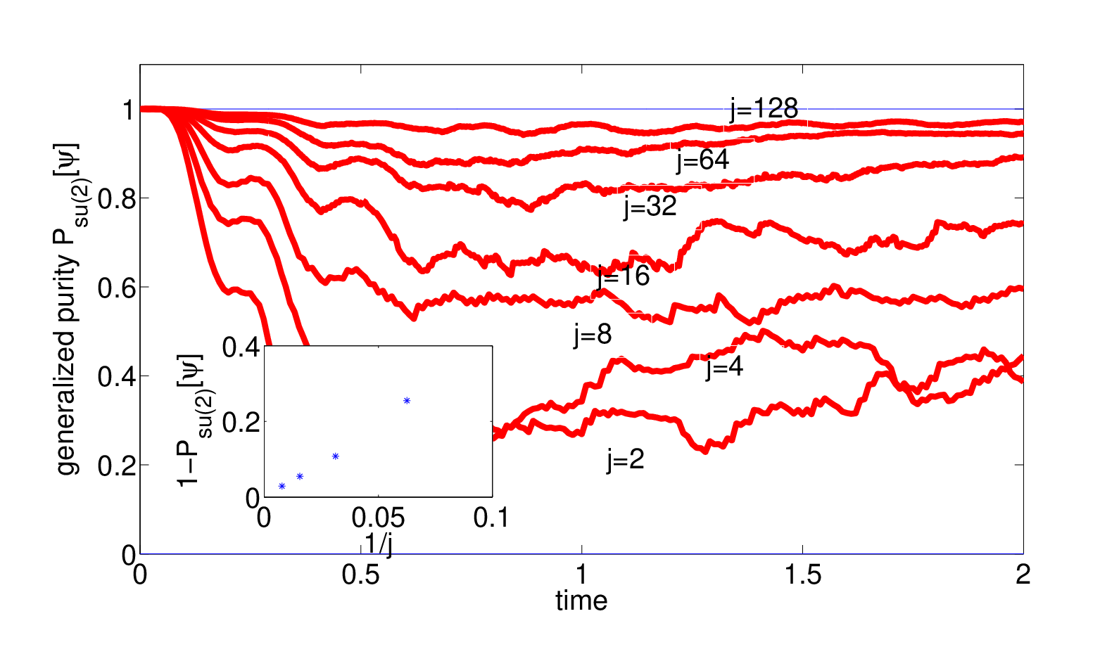
Fig. (1) displays the evolution of the expectation values of the operators ${{\mathrm{\hat{J}}}}_{x}/j$, ${{\mathrm{\hat{J}}}}_{y}/j$ and ${{\mathrm{\hat{J}}}}_{z}/j$ in the unitary evolution $\gamma=0$ and in the nonunitary case $\gamma=0.05/j$ for $N=2j=128$ particles in the condensate. The hopping rate $\omega=15$ and the strength of the on-site interaction is $U=\omega/2j$. It can be seen that the evolution is negligibly perturbed by the bath for the chosen strength of the coupling $\gamma$. We also plot the generalized purity of the unitarily evolving state and of a random stochastic unraveling of the nonunitary evolution. The generalized purity in the unitary case decreases to the value of about 0.06, which corresponds (Appendix A) to the number of configurations $M=0.75(2j+1)\approx 100=O(N)$ in the GCS expansion of the solution. On the other hand, the generalized purity in the stochastic unraveling is about $0.9-0.95$ which corresponds to a drastic reduction of the number of configurations to $M=0.04(2j+1)\approx 5\ll N$.

An interesting feature of the stochastic evolution displayed on Fig.(1) (and observed in other numerical simulations, see Fig.(2)) is that apparently, the generalized purity approaches a constant value on average. Since the generalized purity is a measure of localization of the state on the corresponding phase space (which is the Bloch sphere for the ${\mathfrak{su}}(2)$ algebra [26, 13, 27]) such behavior is suggestive of a soliton-like solution of the sNLSE (26). Investigation of existence and properties of these soliton-like solutions seems to be an interesting topic for future research. For the time being let us assume that the stationary (on average) value $P$ of the generalized purity as displayed on Fig.(1) is an analytical function of $1/j$ (see Fig.2 for some evidence). Then

$\displaystyle P=1-\frac{1}{j}f(\omega^{a}U^{b}\gamma^{c}),$

(41)

to the lowest order in $1/j$, where $f$ is an unknown function of the dimensionless argument $\omega^{a}U^{b}\gamma^{c}$ and $a+b+c=0$. Using the estimate (Appendix A) for the number of configurations we obtain

$\displaystyle M=(2j+1)(1-\sqrt{P})=f(\omega^{a}U^{b}\gamma^{c}),$

(42)

i.e., the number of configurations in the expansion of the stochastic unraveling does not depend on $j$. Numerical evidence implies that generally $f(\omega^{a}U^{b}\gamma^{c})\neq 1$. For example, the value of $f(\omega^{a}U^{b}\gamma^{c})$ deduced from the Fig. 2 is three. This implies, that asymptotically, as $j\rightarrow\infty$, the dynamics of the single-particle observables of the two-modes Bose-Hubbard model can be reproduced not by an averaging over stochastic GCS evolutions (stochastic mean-field solutions), but rather by an averaging over the stochastic evolutions of superpositions of a constant small number $M>1$ of GCS.

The current observations were also found in different parametric regimes of the Bose-Hubbard model. Similar behavior has been observed in the study of the ${\mathfrak{su}}(2)$-Hamiltonians, such as the Lipkin-Meshkov-Glick model [28] of a system of interacting fermions.

The novel strategy for efficient simulation of a unitary evolution of a restricted set of observables has been outlined (Cf. Fig.3). The restricted set comprises the spectrum-generating Lie-algebra of the system. The unitary evolution of the observables is simulated by a particular open-system dynamics, corresponding to the process of weak measurement of the observables, performed on the evolving quantum system. The scheme is based on a large time-scales separation between the decoherence of the evolving state in the basis of the generalized coherent states (GCS), associated with the algebra, and the relaxation of the elements of the algebra. The necessary condition for the successful implementation of the algorithm is the ”classicality” condition on the spectrum-generating algebra and its Hilbert space representation. This time-scale separation is proved for linear Hamiltonians and it is conjectured that the time-scales separation is preserved if the Hamiltonian is at most bilinear in the elements of the algebra. Numerical evidence obtained in the ${\mathfrak{su}}(2)$ case supports the conjecture. The ”classicality” condition excludes efficient simulation of certain subalgebras of observables (Appendix B). For example, the unitary dynamics of local observables of a composite system of qubits cannot be simulated with higher efficiency by the open-system evolution.

The fast decoherence reduces the computational complexity of the evolution, while the slow relaxation leaves the dynamics of the restricted set of observables practically unaffected on physically interesting time-scales. The effect of a fictitious coupling to a bath can be viewed as a dynamically induced coarse-graining of the evolving state in the phase-space, associated with the spectrum-generating Lie-algebra. The fine structure of the evolving state, irrelevant for the expectation values of the ”smooth” observables, is rubbed out by the decoherence, thereby reducing the computational complexity of the evolution. This coarse-graining can be seen as a generalization of the process of conversion of quantum correlations (entanglement) to classical correlations under the action of local dephasing environments [29]. The reduction of the computational complexity is realized by simulating the stochastic nonlinear Schrödinger equation (sNLSE), governing the stochastic unraveling of the nonunitary evolution. The GCS are globally stable solutions of the sNLSE, corresponding to an Hamiltonian, linear in the algebra elements [20]. Numerical evidence obtained in the ${\mathfrak{su}}(2)$ case suggests that Hamiltonians bilinear in the generators asymptotically lead to soliton-like stable localized solutions of the corresponding sNLSE. Averaging over the stochastic realizations of the open-system evolution recovers the unitary dynamics of the restricted set of observables. It is proved that the averaging can be performed efficiently, provided that the observables can be efficiently measured in an experiment.

The fictitious bath is fine-tuned $-$ it corresponds to a process of weak measurement of the orthonormal basis set of the operators, performed with equal rates and strengths. This fine-tuned bath is constructed as a computational tool. On the other hand, if the fine-tuning condition is dropped, the resulting open-system dynamics can represent a real physical situation, where the linear part of the Hamiltonian is perturbed by the time-dependent $\delta$-correlated noise [30]. In that case the density operator of the system will follow an open evolution, corresponding to a process of weak measurement of the algebra elements, performed with generally different rates [30]. It is expected, that if the noise is sufficiently weak, the constant part of the Hamiltonian will induce fast (on the relaxation time-scale) rotation in the Hilbert-Schmidt operator space, which effectively will average out the difference between the contributions of various measurements. Therefore, this real bath is expected to induce the same type of localization as the fine-tuned fictitious bath. Numerical evidence obtained in the ${\mathfrak{su}}(2)$ case supports this conjecture [23]. Restricting the measurements to the algebra elements, the experimentalist will not observe the effect of the bath if the noise is sufficiently small, while measuring the higher order correlations will reveal the nonunitary character of the evolution. Generally, it is expected that the resulting open-system dynamics can be simulated with higher efficiency than the corresponding unitary dynamics, provided the ”classicality” condition holds.

The main open questions to be addressed are:

• •

  Investigation of the effect of nonlinear terms in the Hamiltonian (1) on the relaxation time-scales of the observables in the spectrum-generating algebra in the corresponding fictitious open-system dynamics, Eq.(3).

• •

  Development of an efficient and convergent algorithm for simulating the evolution of a state in the GCS basis representation.

• •

  A rigorous proof of the conjecture, that for Lie-algebraic Hamiltonians, bilinear in the generators, Eq.(1), the generalized purity of the stochastic unraveling of the corresponding open system evolution, Eq.(3), is stationary on average and the stationary purity approaches a limiting value independent on the dimension of the Hilbert space if the classicality condition becomes stronger.

References

- [1] Ronnie Kosloff, J. Phys. Chem. 92, 2087 (1988).
- [2] A. Bohm, Y. Neeman and A. O. Barut, Dynamical groups and spectrum generating algebras (World Scientific, Singapur, 1988).
- [3] R. Gilmore, Lie groups, Lie Algebras and Some of Their Applications (John Wiley and Sons, New York, 1974).
- [4] F. Iachello and R. Levine, Algebraic Theory of Molecules (Oxford University Press, Oxford, 1995).
- [5] F. Iachello, Lie Algebras and Applications (Springer, Berlin, 2006).
- [6] G. Lindblad, Comm. Math. Phys. 48, 119 (1976).
- [7] H.-P. Breuer and F. Petruccione, Open quantum systems (Oxford university press, 2002).
- [8] L. Diosi, Weak measurements in quantum mechanics (v 4, p276-282 in: Encyclopedia of Mathematical Physics, eds.: J.-P. Fransoise, G.L. Naber, and S.T. Tsou , Elsevier, Oxford, 2006).
- [9] N. Gisin, Phys. Rev. Lett. 52, 1657 (1984).
- [10] L. Diosi, Physics Letters A 129, 419 (1988).
- [11] N. Gisin and I. C. Percival, J. Phys A: Math.Gen. 25, 56775 (1992).
- [12] A. Perelomov, Generalized Coherent States and their Applications (Springer, Berlin, 1985).
- [13] W. Zhang, D. H. Feng and R. Gilmore , Rev. Mod. Phys. 62, 867 (1990).
- [14] T. Schumm, S. Hofferberth, L.M. Andersson, S. Wildermuth, S. Groth, I. Bar-Joseph, J. Schmiedmayer, P. Kruger, Nature Physics. 1, 57 (2005).
- [15] R. Gati, B. Hemmerling, J. Folling, M. Albiez, M. K. Oberthaler, Phys. Rev. Lett. 96, 130404 (2006).
- [16] R. Delbourgo and J. R. Fox, J. Phys A: Math.Gen. 10, L233 (1977).
- [17] H. Barnum, E. Knill, G. Ortiz and L. Viola , Phys. Rev. A 68, 032308 (2003).
- [18] A. A. Klyachko, (e-print, quant-ph/0206012).
- [19] S. Boixo, L. Viola and G. Ortiz, EPL 79, 40003 (2007).
- [20] M. Khasin and R. Kosloff (arXiv: 0804.1103v1).
- [21] L. Viola and W. G. Brown, J. Phys A: Math.Gen. 40, 8109 (2007).
- [22] R. Somma, H. Barnum, G. Ortiz and E. Knill, , Phys. Rev. Lett. 97, 190501 (2006).
- [23] M. Khasin and R. Kosloff, in preparation.
- [24] P. Kramer and M. Saraceno, Geometry of the Time-Dependent Variational Principle in Quantum Mechanics (Springer-Verlag, Berlin, 1981).
- [25] A. Vardi and J. R. Anglin, Phys. Rev. Lett. 86, 568 (2001).
- [26] F.T. Arecchi, E. Courtens, R. Gilmore and H. Thomas, Phys. Rev. A 6, 2211 (1972).
- [27] V.R. Viera and P.D. Sacramento, Ann. Phys. 242, 188 (1995).
- [28] H. J. Lipkin, N. Meshkov and A.J. Glick, Nucl. Phys. 62, 188 (1965).
- [29] M. Khasin and R. Kosloff, Phys. Rev. A 76, 012304 (2007).
- [30] V. Gorini and A. Kossakowski, J. Math. Phys. 17, 1298 (1976).
- [31] I. Tikhonenkov, J. R. Anglin and A. Vardi, Phys. Rev. A 75, 013613 (2007).
- [32] F. Trimborn, D. Witthaut and H. J. Korsch (arXiv:0802.1139v1).