A secular theory of coplanar, non-resonant planetary system
Abstract
We present the secular theory of coplanar -planet system, in the absence of mean motion resonances between the planets. This theory relies on the averaging of a perturbation to the two-body problem over the mean longitudes. We expand the perturbing Hamiltonian in Taylor series with respect to the ratios of semi-major axes which are considered as small parameters, without direct restrictions on the eccentricities. Next, we average out the resulting series term by term. This is possible thanks to a particular but in fact quite elementary choice of the integration variables. It makes it possible to avoid Fourier expansions of the perturbing Hamiltonian. We derive high order expansions of the averaged secular Hamiltonian (here, up to the order of 24) with respect to the semi-major axes ratio. The resulting secular theory is a generalization of the octupole theory. The analytical results are compared with the results of numerical (i.e., practically exact) averaging. We estimate the convergence radius of the derived expansions, and we propose a further improvement of the algorithm. As a particular application of the method, we consider the secular dynamics of three-planet coplanar system. We focus on stationary solutions in the HD 37124 planetary system.
Keywords:
celestial mechanics – secular dynamics – analytical methods – stationary solutions – extrasolar planetary systems – stars: HD 371241 Introduction
The recent discoveries of extrasolar planetary systems bring new and interesting problems regarding their dynamical stability and long-term evolution. At present, at least 30 multi-planet systems are known and their number is still growing, thanks to refined techniques of observations. Surprisingly, the orbital parameters of these systems are very different from those typical in the Solar System architecture — large planetary masses and eccentricities are common. Simultaneously, these systems usually are compact. Likely, this property is a consequence of the observational selection. The most effective detection techniques, like the radial velocity observations, rely on indirect effects of mutual interactions between planets and their host star. Many of the known multi-planet systems are supposed to be involved in short-term mean motion resonances (MMRs). However, there are also configurations with relatively well separated orbits. In that case the secular interactions may lead to interesting dynamical phenomena.
To study the long term dynamics of planetary systems, different analytical and numerical techniques are used. The analytical approach is much more effective in the investigations of global, qualitative dynamics than widely applied numerical techniques (including fast indicators or direct numerical integration of the equations of motion). The numerical experiments provide only limited (or local) information on the dynamical features of the studied configurations. Usually, the interpretation of the results of massive calculations can be problematic without solid theoretical background. In contrast, analytical techniques offer much deeper insight into qualitative properties of motion. The analytical approach makes it possible to explore large volume of the phase space. This is crucial for the dynamical studies of extrasolar planetary systems detected during short time of observations. These observations have relatively large errors, they are typically irregularly sampled or degenerated (in the sense that they can provide only limited information on the system state, like the radial velocity technique). This leads to poorly determined or unconstrained orbital and physical parameters of the detected systems. In that case, the analytical theories help us to investigate and/or to detect global properties of the solutions to the equations of motion in observationally permitted ranges of the parameters. We can investigate in detail certain families of these solutions, their bifurcations and stability. Examples of such solutions are stationary solutions (equilibria) or periodic orbits that build a skeleton of the phase space. Investigating these families, we follow the classic methodology invented by Poincaré. The analytical theories are milestones for detailed numerical studies of particular aspects of the dynamics. Hence, their constant development is always desirable.
Moreover, due to extreme parameters of the studied configurations, the classic planetary theory developed so far is often too week. For instance, the classic Lagrange-Laplace theory (Murray & Dermott, 2000) designed as a model of the secular dynamics of planets in the Solar System fails in the case of large eccentricities and inclinations. Hence, new analytical and semi-analytical theories are recently developed, breaking the limitations of the classic approach. One of the most effective techniques for studying the secular dynamics of extrasolar systems has been recently invented by Michtchenko & Malhotra (2004) and further developed in (Michtchenko et al., 2006). These papers are devoted to a study of two-planet configurations. In this work, we consider an analytical secular theory of a coplanar system of -planets (point masses) under assumption that the orbital configurations are not involved in strong mean-motion resonances and that they are far from collisions zones of orbits. We calculated the averaged perturbation in the form of power series with respect to the semi-major axes ratios up to very high order (equal to 24 in the present work). These expansions have no explicit limits on the eccentricities provided that the non-resonance condition is satisfied. Our development is elementary and is based on very basic properties of the Keplerian motion. Although it concerns the two-planet system, we show that it can be easily generalized for the case of -planet configurations. Hence, the theory can be regarded not only as an attempt to improve the secular theories for two-planet systems in (Rodríguez & Gallardo, 2005; Henrard & Libert, 2005; Libert & Henrard, 2005; Libert & Henrard, 2006; Ji et al., 2007; Veras & Armitage, 2007, e.g.,), relying on the classic expansion of the perturbing Hamiltonian in eccentricities (Murray & Dermott, 2000; Ellis & Murray, 2000) or the octupole theory that makes use on the averaging of the low-order expansion of the perturbing function in the semi-major axes ratio (Ford et al., 2000; Blaes et al., 2002; Lee & Peale, 2003). We try to reduce the limitations of the classic theory of non-resonant systems.
The plan of this paper is as follows. In Section 2, we describe a general model of a coplanar configuration of planets. We introduce the expansion of perturbing Hamiltonian and a very simple and basic algorithm of its averaging. We compare the results of the method with the outcome of the octupole theory, and we discuss some subtle differences between these theories. We also present the results of the tests of the expansion, taking as examples a few known multi-planet configurations which apparently fit well in the framework of the non-resonant secular theory. The exact semi-numerical method is helpful to determine absolute bounds of the validity of the analytic approach. We also outline a further improvement of the averaging algorithm. In Section 3 we construct the secular model of the three-planet system and we perform a preliminary study of the secular dynamics of a few known three-planet configurations. In particular, we focus on the equilibria in the secular problem, and we found interesting stationary solutions in the extrasolar system HD 37124 (Vogt et al., 2005; Goździewski et al., 2008).
2 The secular dynamics of a multi-planet system
The Hamiltonian of a multi-planet system with respect to canonical Poincaré variables (Laskar & Robutel, 1995; Michtchenko & Malhotra, 2004, see, e.g.,) can be expressed by a sum of two terms,
| (1) |
where
| (2) |
is for the integrable part comprising of the direct sum of the relative, Keplerian motions of planets and the host star. Here, the dominant point mass of the star is , and , are the point masses of the -planets. For each planet–star pair we define the mass parameter where is the Gauss gravitational constant, and are the so called reduced masses. Due to mutual interactions between the planets, the Keplerian part is perturbed by a function ,
| (3) |
where are for the position vectors of the planets relative to the star, are for their conjugate momenta relative to the barycenter of the whole -body system, denote the relative distance between planets and . It is well known that even in the simplest case of three point masses (the star and two mutually interacting planets), the problem is non-integrable and is not possible to obtain its exact analytical solutions. In practice, such solutions can be only derived in the form of approximations derived by means of different perturbation techniques (Murray & Dermott, 2000; Morbidelli, 2002; Ferraz-Mello, 2007, e.g.,).
To apply the canonical perturbation theory, we first transform to the following form:
| (4) |
where stand for the action-angle variables, and , where is a small parameter. In the absence of this perturbation, the system is trivially integrable. However, with the perturbation added, the dynamics of the full system become extremely complex. In the realm of the Hamiltonian canonical theory, the approximate, analytical solutions to this problem may be derived by an expansion of the perturbation with respect to the small parameter and by subsequent simplification of the lowest order terms by means of appropriate canonical contact transformations. This idea of Delaunay appears in many “incarnations”. One of its first novel realizations is known as the von Zeipel method (Brumberg, 1995, e.g.,). Much more improved version of this technique that not require series inversion has been invented by Hori (1966) and next refined by Deprit (1969). This theory is well known in the literature as the Lie-Hori-Deprit method. For an excellent review of these methods see a monograph by Ferraz-Mello (2007). Another method of seeking for approximate solutions to Eq. 4 relies directly on the averaging proposition (Arnold et al., 1993, see, e.g.,). Usually, the canonical angles can be divided onto two classes: fast and slow ones. By averaging the perturbing part with respect to the fast angles over their periods, we obtain the secular perturbation Hamiltonian which does not depend on these fast angles. Simultaneously, their conjugate momenta become integrals of the secular problem. In the planetary model with a dominant stellar mass, we have two natural time-scales of motion: the orbital motion of the planets and a slow evolution of their orbits. Assuming that no strong mean motion resonances are present, and the system is far enough from collisions, the averaging makes it possible to reduce the number of the degrees of freedom and to obtain qualitative information on the long-term changes of the slowly varying orbital elements (i.e., on the slow angles and their conjugate momenta).
To apply each one of these methods, the Hamiltonian of the -planet system should be first transformed to the required form, Eq. 4. This can be accomplished by expressing it with respect to the canonical Poincaré elements (Murray & Dermott, 2000; Michtchenko & Malhotra, 2004):
| (5) | |||||
where are the mean longitudes, stand for canonical semi-major axes, are for the eccentricities, denote inclinations, are the longitudes of pericenter, and denote the longitudes of the ascending node. We note that the transformation between the canonical orbital elements of Poincaré, , , , , and associated Cartesian coordinates and momenta may be derived by the formal two-body transformation between classic (astro-centric) Keplerian elements and the Cartesian coordinates (Morbidelli, 2002; Ferraz-Mello et al., 2006, e.g.,). Moreover, in the settings adopted here, the rectangular coordinates and momenta are understood through the Cartesian positions of planets relative to the star, and, according to the definition of the Poincaré variables, the canonical momenta are taken relative to the barycenter of the system.
The -body Hamiltonian expressed in terms of the Poincaré variables has the form of:
In this Hamiltonian, play the role of the fast angles. In the absence of strong MMRs, these angles can be eliminated by the following averaging formulae:
| (6) |
(As we see below, it can be also applied for some selected pairs of planets). Hence, the conjugate momenta become integrals of the secular model and the Keplerian part is a constant that does not contribute to the equations of motion. However, the calculation of the multiple integral is quite a difficult task which is a central part of the problem. We try to solve it with quite basic mathematical properties of the Keplerian osculating orbits.
We should keep in mind that the averaging of the secular Hamiltonian in the problem over Keplerian motions implies truncation of the perturbation to first order in the masses (more generally, to the first order in the perturbation parameter ). For large mutually interacting planets (or binary stars), the deviations of the true orbits from the Keplerian approximation during the orbital period may become significant, and the secular theory may fail. Nevertheless, it is a common drawback of the idea behind Eq. 6. For the same reason, the classic perturbation techniques usually fail in the case of close encounters between the planets. In such an instance, some other criteria helping to explore the stability regions may be applied, for example, the Hill stability criterion (Marchal & Bozis, 1982; Gladman, 1993; Barnes & Greenberg, 2006; Michtchenko et al., 2008; Barnes & Greenberg, 2008).
2.1 The indirect part of the disturbing function
We start with the averaging of the indirect part of the disturbing Hamiltonian. The result of this averaging can be found in Brouwer & Clemence (1961), nevertheless, to make this paper self-consistent, we present the calculations in detail. The indirect part is a scalar product of canonical momenta , which have the form of:
| (7) |
where and is the total mass of the system. The scalar product includes terms of the type of . Moreover, each product depends on all astro-centric velocities of the planets, (). Apparently, to average out the indirect part of the disturbing function, we must compute multiple integral over all mean longitudes (). In fact, this integral can be reduced to a sum of double integrals computed for all pairs of planets, i.e., we average out expressions of the form of . The result is the following:
| (8) |
where denote mean motions of the planets and stands for the Kronecker delta. Note, that the averaging over the mean anomalies gives the same results as the averaging over the mean longitudes under the condition that the integration limits are set to and , respectively. Clearly, the indirect part of the disturbing function does not contribute to the secular dynamics of the system because it depends on only (Brouwer & Clemence, 1961), (Michtchenko & Malhotra, 2004, see also). We note that this result is exact as far as the assumptions of the averaging principle are fulfilled (we are far enough from the MMRs and there are present two different time-scales in the problem).
2.2 The direct part of the disturbing function
Now we have a more difficult problem to resolve. For the -planet system, the averaged direct part of the disturbing function has the form of:
| (9) |
where the multiple integral Eq. (6) over all mean anomalies is reduced to a sum of secular Hamiltonians describing mutual interactions between all pairs of planets; i.e., for each pair , where and , we have:
| (10) |
Hence, the secular model of -planet system can be reduced to a simple sum of two-planet Hamiltonians.
Now, we compute the double integral for a fixed pair of planets and . The distance between these planets is the following:
| (11) |
where is the angle between vectors and :
| (12) |
This formulae can be rewritten to:
| (13) |
According to the Kepler problem theory, and may be expressed through the eccentric anomaly, , or, equivalently, through the true anomaly, . We write down appropriate expressions for planet and , respectively:
Here, is the eccentric anomaly of the inner planet in the selected pair of interacting bodies, and is the true anomaly of the outer planet. Moreover:
where , and
The dependence of the two-body formulae on may seem strange. However, when we investigate the co-planar system of two particular planets, we are free to choose the reference frame because the mutual interaction between these planets depend only on their relative orbital phases. To be more specific, we must calculate the distance between planets and , or the scalar product (Eq. 11). That is obviously independent on the reference frame. In general, we could write:
| (14) |
where are the orbital reference frames of the inner and outer planet, respectively, matrices represent Eulerian rotations of to a common reference frame () for both orbits. Because this frame may be chosen freely, we fix the -direction of the common frame along the apsidal line of the inner planet (still, for a particular pair of planets). Then and must be rotated by angle . That can be repeated for each pair of planets in multi-planet system because the secular Hamiltonian is represented by a sum of formally independent two-planet terms.
Finally, the inverted distance between planets can be expressed as follows:
where , and
| (15) | |||||
| (16) | |||||
Now we underline that the position of the inner planet is given through the eccentric anomaly while the position of the outer planet is given with respect to the true anomaly. The formulae under the square root are expressed by a polynomial of trigonometric functions and, as we can see below, that is critically important property making it possible to calculate the integral in Eq. 10.
Now, we expand the inverse of the distance between planets and in Taylor series with respect to small parameter . The series are evaluated around as follows:
| (17) |
where
| (18) |
As the final result of this expansion, we obtain a polynomial with respect to trigonometric functions of the anomalies which has the general form of:
| (19) |
Here, is a vector of natural numbers and are coefficients depending on eccentricities and semi-major axes. One more step is still necessary. The integral in Eq. 10 must be computed with respect to the mean anomalies. Here, the classic theories make use on and expressed through Fourier series of the mean anomalies with coefficients dependent on the eccentricities.
However, we found that it is possible to avoid these expansions. Again, using the basic formulae of the Keplerian motion, we perform a formal change of variables in Eq. 10 with: and , where functions and are defined with:
| (20) |
After this change of variables, the average in Eq. 10 is equivalent to calculation of the following double integral:
| (21) |
where .
Fortunately, functions are again trigonometric polynomials and they do not change the general, polynomial form of Eq. 19. However, the second scaling function is not a polynomial with respect to or . Yet Eq. 17 involves a factor . It cancels out one power of appearing in the denominator of Eq. 20. In order to calculate the expansion in Eq. 17, for we differentiate with respect to as the composite function (Eq. 18). This operation emerges factors of the type of , where . Looking at the general form of and we see that the term appears with natural powers larger than and it cancels out remaining in the denominator of Eq. 20. In this way, the general form of trigonometric polynomial in Eq. 19 is preserved. Still, the free term in the Taylor expansion of leads to an expression involving . Fortunately, we must integrate such term with limits from to and this effectively can be reduced to averaging out over the orbital period (or the whole range of the true anomaly).
Finally, we can integrate Eq. 21 term by term. Basically, the problem has been reduced to the calculation of definite integrals from products of trigonometric functions and in some natural powers. These integrals can be derived quite easily, at least in principle, nevertheless with increasing order of the Taylor expansion, the calculations become extremely tedious. To accomplish them, we used MATHEMATICA and fast AMD-Opteron computer.
The final result of the averaging is an expansion of the secular, two-body Hamiltonian for a chosen pair of planets and :
| (22) |
Looking at the general form of this secular Hamiltonian, we learn that the role of a formal parameter in the power-series expansion of plays (apparently) the following expression:
| (23) |
Obviously, these series cannot converge if , hence we require that . Of course, this is only the necessary (and as we see below, very rough) condition for the convergence of these series. However, as we explain in Sect. 2.5, attributing to the role of a parameter deciding on the convergence of these series is in fact misleading because their divergence flows from quite a different source.
A few first terms of the expansion of the secular Hamiltonian, Eq. 22, are listed below. The free term (for ) is constant because it depends on the mean semi-major axis only. The term with vanishes identically.
Terms of order and may be identified with the quadrupole and octupole secular Hamiltonian, respectively (Ford et al., 2000; Lee & Peale, 2003):
| (24) | |||
| (25) |
Higher order terms are the following:
| (26) | |||
| (27) | |||
| (28) | |||
We computed the expansion up to the order of 24. This expansion is available on the request in the form of raw MATHEMATICA input file; also available in the form of on-line material after publishing this paper.
2.3 A comparison with the octupole theory
Here, we compare the results provided by the secular theory derived in the previous section with the results obtained with the help of the octupole theory of two planets (Lee & Peale, 2003) which has been obtained through averaging the perturbation Hamiltonian with the help of von Zeipel method up to the third order in . It has been applied to study qualitative features of the secular dynamics in hierarchical planetary systems (i.e. with small ). A similar theory has been developed by Ford et al. (2000) who investigated secular dynamics in hierarchical triple stellar systems with large separation of the third body.
To make our discussion more transparent, we use, in this section, the notation of Lee & Peale (2003). Their equations (13), (14) and (15) have the following form:
| (29) | |||
| (30) | |||
| (31) |
where are planetary masses, is the mass of the star, (we set the gravitational constant to ). To derive the octupole theory in terms of Jacobi reference frame, we start from writing down Eq. 1 with respect to Jacobi coordinates of two point masses, as a sum of two Keplerian terms and the perturbation:
where
Here, are the conjugate Jacobi momenta, , and the reduced masses are
For details, see, e.g., (Malhotra, 1993). Now, after expanding with respect to small and retaining first order terms, we can show that the perturbation has the same form as Eq. 3 with the accuracy to the second order in the masses (Malhotra, 1993):
The same truncated Hamiltonian is analyzed in (Libert & Henrard, 2005) who derived the secular Hamiltonian of the 12-th order in eccentricities by the ”averaging with scissors” (i.e., by eliminating from the Fourier expansion of all fast periodic terms dependent on ). These authors report that their secular theory reproduces qualitatively results of Michtchenko & Malhotra (2004) on the analytical way.
The indirect part of the truncated Hamiltonian also averages out to a constant, hence the rest of the averaging process is the same as in the case of written with respect to the Poincaré elements. Nevertheless, the averaged is missing terms of orders higher than two in the planetary masses. Indeed, with our method we derived the secular octupole Hamiltonian which has the same functional form as formulae (17) in (Lee & Peale, 2003). However, there are some differences in coefficients and [see their equations (18) and (19)]. These coefficients in our expansion are the following:
| (32) | |||
| (33) |
where we extracted out two factors leading to the difference between the respective formulae:
| (34) | |||
| (35) |
These factors can be thought as equal to in (Lee & Peale, 2003). However, the theories are consistent within the assumed accuracy of the expansion and the relative magnitude of terms skipped from [of the order of ].
Actually, our averaging algorithm can be applied also to the full perturbing Hamiltonian, thanks to straightforward generalization for terms like the following:
where are some constants. In that instance, we obtain exactly the same as in (Lee & Peale, 2003). Hence, as one would expect, both approaches lead to fully equivalent results.
This comparison also reveals that the averaging of the truncated Hamiltonian is in fact quite problematic because the accuracy of the secular expansion has nothing to do with the magnitude of the rejected terms. Already for Jupiter-mass planets, a contribution of these terms may be significant (see Sect. 2.4 for details).
Moreover, a direct comparison of the theories would be more subtle. Although the functional forms of the perturbing Hamiltonians are the same, they are expressed in terms of two different sets of canonical variables. Hence, the mean elements have different meaning in these theories, i.e., the same physical configuration of the planets will be parameterized with quantitatively different values of the mean elements.
2.4 Tests of the analytic secular theory
To test the accuracy and relevance of the high order expansion of , we calculated the magnitude of subsequent terms relative to the free term. This expansion is computed up to the order of 24 for parameters () of extrasolar planetary systems taken from the Jean Schneider Encyclopedia of Extrasolar Planets11 1 http://exoplanets.eu. The results of this experiment are presented in Fig. 1. Each panel in this figure is labeled with the name of a relevant star and a number of putative planets it hosts (written in brackets). As we can see, for all examined systems, the sum of terms in of the same order (note that we can have two and more planets in the system) decrease rapidly with the order of the expansion. For a few most separated systems with two planets (e.g., HD 217107, HD 190360), the highest order terms are as low as in the relative magnitude. In the tested sample, the largest 24th-order terms are . Hence, the secular energy can be calculated with excellent accuracy. We note that similar tests of the precision of the secular theory were presented in (Rodríguez & Gallardo, 2005) and (Libert & Henrard, 2005).

In the second test, we compare the outcome of our algorithm with the results of semi-analytical approach by Michtchenko & Malhotra (2004); Michtchenko et al. (2006) [see also Migaszewski & Goździewski (2008a) for some technical aspects] who applied the method to study the secular dynamics of two-planet system. In the algorithm of Michtchenko & Malhotra (2004) the perturbing Hamiltonian is averaged out by means of the numerical integration. Hence, one avoids any expansion of the Hamiltonian and the results are formally exact (or very accurate, providing that precise enough quadratures are applied).
To examine the accuracy of the analytic secular theory, we calculated the levels of the secular Hamiltonians for a number of extrasolar planetary systems which can be potentially regarded as non-resonant or well fitting assumptions of the secular theory. Because the phase space of the secular problem is three-dimensional [i.e., ], we choose the so called representative plane of the initial conditions to plot the secular energy levels. The definition of the representative plane follows Michtchenko & Malhotra (2004). The secular Hamiltonian of a coplanar two-planet system depends only on and eccentricities coupled through the integral of the total angular momentum (or the so called Angular Momentum Deficit, ). Effectively, the secular problem has one degree of freedom and is integrable. Michtchenko & Malhotra (2004) have shown that all phase trajectories of the non-resonant system pass through a plane defined with or [see also (Pauwels, 1983) for the qualitative analysis of the secular two-planet problem]. The representative plane may be defined for fixed and as follows:
This plane comprises of two -half-planes with for and with for . Simultaneously, the derivatives of the secular Hamiltonian with respect to are equal to zero for . It follows from the symmetry of interacting orbits with respect to both apsidal lines. Having the secular Hamiltonian in explicit analytic form, we can verify this property directly. Indeed, each term in the secular Hamiltonian depends on only through with , and it means that is even function of . Hence, implies factors involving and these terms vanish identically for . Formally, it is possible that also for , however, to find such solutions we should solve highly nonlinear equation involving and trigonometric functions of .
Each pair of for which corresponds to an equilibrium in the secular problem (simultaneously, they are the extrema of the secular Hamiltonian). These equilibria appear both in the negative half-plane of , as mode II solutions (this mode is Lyapunov stable, and may be characterized with librations of angle around in the evolution of neighboring orbits), and in the positive half-plane of as mode I solutions (Lyapunov stable, with librations of angle around of the nearby orbits). Further, in the regime of large eccentricities, in the positive half-plane a new, non-classic mode of motion may appear [it is the so called non-linear secular resonance, NSR from hereafter, see (Michtchenko & Malhotra, 2004) for details]. These results are derived through the numerical (exact) approach, hence their reproduction by the analytical theory provides an absolute test of its quality and accuracy.


The results of the second experiment are presented in Figure 2. Each panel in this figure is for the representative plane of initial conditions computed and calculated for two-planet systems characterized with mass ratio and semi-major axes ratio . These parameters are written in the top-left corner at each relevant panel. To illustrate the significance of highest order terms in Eq. 22, we plot contour levels of , i.e., the relative magnitude of the sum of the last two terms with respect to the magnitude of the free term (in general, would stand for a sum of expansion terms over the number of planet pairs in the given multi-body configuration). Four particular contour levels of , , and , respectively, are distinguished with thicker lines and labeled accordingly.
In each panel, we also marked positions of stationary solutions (modes I, II, and NSR). Solutions represented by thick curves are derived with the help of numerical averaging (Michtchenko & Malhotra, 2004): blue curves are for stable equilibria, and thick green curves are for unstable solutions (the non-linear secular resonance). These curves represent practically exact (or very precise) solution to the problem. The thin, red lines mark the positions of equilibria calculated analytically, with the help of the th-order expansion of .
The results can be summarized with a few interesting conclusions. Clearly, in the regions of the representative -plane at which , the precision of the analytical method is excellent. The secular theory predicts exactly positions of the equilibria in the negative half-plane of (when ) no matter how large is . On contrary, the exact derivation of the shape of the non-linear secular resonance is a challenging problem for the analytic approach (Henrard & Libert, 2005, see also). The nonlinear resonance can be reproduced well by the analytic theory providing that . This is also an empirical border of the convergence of the secular expansion. We also found another empirical convergence condition that follows from the notion of the geometric series, i.e, This inequality is illustrated with triangular, orange colored regions labeled with “”. In these regions, the series are divergent, hence the secular theory cannot reproduce the real dynamics. This may be interpreted as a clear limitation of the analytic theory. In fact, as we show below (Sect. 2.5), this problem appears rather due to imperfect algorithm of the expansion, which can be still improved. On the other hand, the results of this test provide an example that illustrates excellent properties of the semi-analytical approach invented by Michtchenko & Malhotra (2004).
2.5 An improved averaging algorithm
A real source of the divergence of the secular series, Eq. 22, can be deduced after we draw in Fig. 2 the “anti-collision” line defined through (see the right-half of the representative plane). Clearly, the series diverge above this line and the positions of the equilibria are strongly distorted. In this area, for some points or parts of the orbits, , while in the expansion Eq. 22, must be satisfied in the whole ranges of the anomalies. That may happen when the pericenter of the outer orbit is closer to the star than the apocenter of the inner orbit, no matter what is the relative orientation of their apsidal lines. Then the condition of , which required to write down Eq. 13, is violated. Obviously, it may be expressed by the equation of the anti-collision line, and in other words, through the requirement that the inner orbit lies inside a circle of a radius equal to the pericenter distance of the outer orbit. Now it is also clear why for the apsides anti-aligned, we have always very good convergence of the secular series while in the right half-plane, the convergence region is generally strongly limited. Hence, the convergence limit of the expansion described in Sect. 2 may be simply interpreted through the conditions for the collision lines. We may also note that the problem persists in any secular theory that relies directly on Eq. 13. One should be also aware that the conditions of crossing orbits do not depend on masses. If the masses are large, the dynamical collision curve appears for much smaller eccentricity than the geometrical collision line. (Goździewski et al., 2008; Michtchenko et al., 2008, e.g.,).
A cure for the divergence problem may be a modified expansion of the term , helping us to construct a secular theory that has no limits of the type . To derive the secular expansion in Sect. 2, at first we factor in Eqs. (11), (13). To have the series convergent for all positions of planets on their orbits, we propose to factor from the square root (11) a term consisting of multiplied by some scale factor, (instead of ). Then we can express the distance between planets and as follows:
| (36) |
where
| (37) |
The requirement of the convergent expansion of with respect to implies . If the distance between planets is equal to . The convergence condition is fulfilled when for the given orbits. The maximal distance between planets in coplanar orbits may be bounded by . Then the factor has the form of:
| (38) |
For hierarchical systems with small eccentricity of the outer planet, . For more compact systems with large eccentricities, . For non-coplanar systems, may be even larger. In practice, this parameter makes it possible to control the convergence rate of the secular expansion. The convergence rate will be faster for large distances but slower for smaller distances, moreover the condition of should be always fulfilled.
The term may be expanded with respect to :
| (39) |
To average out the above formulae, we express positions of both planets in a given pair with respect to the eccentric anomaly. Next, we change the integration variables similarly as in Sect. 2, i.e., We also should express through (again, fixing the reference frame with the apsidal line of the inner orbit). After expressing terms through eccentric anomalies, the function has the following explicit form (to shorten the notation, let us fix , for a given pair of planets): :
| (40) | |||
where are eccentric anomalies of the inner and outer planets respectively, and coefficients , read as follows:
| (41) | |||
Here, , and are the eccentricities of the inner and outer planet, respectively.
After the double averaging of over the mean anomalies we obtain:
The averaging of the square of over the mean anomalies brings the following formulae:
| (42) | |||
These preliminary calculations show that the new algorithm leads to more complex expansion of the secular Hamiltonian than the simple approach in Sect. 2.2 which, as we have demonstrated, is limited in some cases. Moreover, we found this improvement after submitting the manuscript, hence the new expansion and a detailed study of its properties would make the paper very lengthy. We are going to present the improved algorithm and the results of its tests in a new work devoted to the analytic theory of non-coplanar model of -planets. A generalization of Eq. 38 for that case seem straightforward, because we should only calculate with the help of appropriate rotation matrix parameterized through Euler angles, i.e., the Keplerian elements (). Hence, only the coefficients will be modified.
3 Secular dynamics of three-planet system
The two-planet secular Hamiltonian in Sect. 2 can be easily adapted to construct the secular theory for -planet system. At present, a few candidates of such configurations are already discovered, including four planet systems, e.g., Arae (Jones et al., 2002; Butler et al., 2006a; Goździewski et al., 2007; Pepe et al., 2007), five or even six planet configuration around 55 Cnc (Fischer et al., 2008). Here, as the simplest and most natural generalization of the two-planet model, we consider the secular theory of -planet configuration which is far from MMRs and collision zones.
The three-planet model is described by Hamiltonian in Eqs. (1), (2) and (3), respectively, where . Because the nodal longitudes are undefined in the coplanar system, and the secular dynamics depends on the relative positions of the mean orbits, we can eliminate the nodal longitudes from the problem. Let indices enumerate the planets. Their semi-major axes are , respectively. After averaging over the mean anomalies, the secular Hamiltonian does not depend on anymore. Therefore, conjugate momenta (hence, the semi-major axes) are constants of motion. Because the secular system does not depend on particular longitudes of nodes, the respective degree of freedom is also irrelevant for the secular dynamics.
Hence, the secular system can be described with the following set of canonical elements:
| (43) | |||
We can eliminate one more degree of freedom with the help of the angular momentum integral, which can be also expressed with . For that purpose, we perform the following canonical transformation:
| (44) | |||
introducing new canonical angles . These angles can be interpreted as two-planet defined for each pair of planets in the three-planet system. The secular Hamiltonian can be expressed through and explicitly, hence is cyclic and is constant of motion. Actually, we reduced the secular system of three planets to two degrees of freedom, with the secular energy and as free parameters.
3.1 Representative planes of initial conditions
Now, we have a similar problem as in the case of two-planet configuration. We want to illustrate the dynamical properties of the system in possibly global manner. To characterize its dynamical states, we follow the general idea of the representative plane of initial conditions. Here, we focus on the equilibria in the secular problem. Fixing the integral of as a parameter of the system, the dynamics may be represented in four-dimensional phase space of , or . The representative plane will be chosen according with:
| (45) |
Then any pair of points that belongs to the representative plane, and the following equations are satisfied:
| (46) |
defines an equilibrium of the secular problem. Note that the last conditions implies also because is a function parameterized by the total angular momentum (or ). The explicit and simple transformation between the eccentricity and the element makes it possible to solve the above conditions in terms of .
Actually, the most obvious definition of the representative plane is a generalization of that plane constructed in the two-planet problem. For fixed , and , as a parameter, the symmetric representative plane is the set of points such that
This plane comprises of four quaters. The signs of of the coordinated axes tell us on the respective values of the secular angles. In that case, the condition in Eq. 45 is fulfilled thanks to apsidal symmetries of the problem. It is also obvious by recalling that is even function of . The derivatives of over depend on factors involving , , that vanish for . Alternatively, the representative plane may be also defined through .
Moreover the condition for the representative plane, defined through the vanishing derivatives over secular angles, may be also fulfilled for . Let us start with the octupole (third-order) approximation of the secular Hamiltonian. Using Eqs. (22), (24) and (25), we can write the secular Hamiltonian in the following short form of:
| (47) |
Using the canonical angles defined with Eq. 44:
| (48) |
where are functions of . Hence, the non-symmetric representative plane is defined through the following conditions, the same as Eq. 45, in the explicit form:
| (49) |
Obviously, conditions in Eq. 49 are satisfied not only when . We have four other solutions, satisfying Eq. 49, i.e.:
| (50) |
These solutions describe the non-symmetric representative planes, with respect to the octupole theory. This definition is exact up to the third order in . Angles satisfying condition in Eq. 45, i.e., solutions to Eq. 49 can be found consistent with higher order expansions. However, these equations are very complex and, in practice, we would have to solve them numerically (for instance, with the Newton-Raphson algorithm initiated with starting conditions derived from the octupole theory). Hence, in general, the representation of the energy levels with the help of the non-symmetric representative planes is much more difficult than in the symmetric case and is not unique (it has some analogy to the Poincaré cross-section). For instance, we can define the representative plane for higher order expansions of . In this paper, we focus on the symmetric representation only.
3.2 Energy levels for three-planet secular model
In this section, to show some applications of the secular theory, we investigate qualitative dynamics of a few three-planet extrasolar systems. To characterize these systems, we calculated energy levels in the symmetric representative plane. We also try to find equilibria in the secular model of each examined system.


The results are illustrated in Figure 3. We selected four three-planet configurations. Their orbital elements are taken from the Extrasolar Planets Encyclopedia of Jean Schneider, following the most recent determinations of the orbital solutions. Each column in Fig. 3 is for one particular system, i.e., for And (Butler et al., 2006b), HD 74156 (Bean et al., 2008), Gliese 581 (Lovis et al., 2006) and HD 69830 (Udry et al., 2007), respectively. Different approximations to the secular theory are illustrated in rows. The top row panels are for the energy levels calculated with the octupole theory, panels in the middle row are derived from the expansion of of the -order, and panels in the bottom row illustrate the energy levels computed with the numerical algorithm. The later case may be regarded as the exact solution to the problem thanks to adaptive, high order Gauss-Legendre quadratures which we used to compute the double integral over . In each case, we fixed consistent with the nominal parameters of the examined systems.
3.2.1 Andromedae
First, we are looking at the exact (numerical) phase plots. In the case of And, we found two types of equilibria. The first one, marked with I, is the global minimum of the secular Hamiltonian. Hence, according to the Lyapunov theorem, this equilibrium is stable (because the Hamiltonian can be regarded as the positive definite Lyapunov function). The equilibrium marked with II is a saddle point, and is stable in the linear approximation. It can be verified by solving the eigenproblem of the linearized equations of motion in the neighborhood of the equilibrium. Now, we can compare the outcomes of the analytic theories with the results of exact, numerical algorithm. Apparently, the high-order analytical theory is fully compatible with the numerical theory. The largest deviations between the secular energies are of the order of . This accuracy is preserved even for eccentricities close to . On contrary, the octupole theory provides only a crude representation of the phase space. The phase plot constructed with the help of this theory also reveals an equilibrium of type I, however, at place of equilibrium II, qualitatively different energy levels appear (see the top-left panel in Fig. 3 with three “false” equilibria).
To locate the “real” system in the energy plot, we mark the level of the secular energy computed for the nominal parameters of the system with green, thick curve. It provides only a crude imagination where the system is located; one should be aware that we are looking at the representative plane (hence are fixed at specific values), and we do not take into account the parameter errors. Still, the plot tell us that while variability of is limited, may be varied in all permitted range of eccentricity.
3.2.2 HD 74156
In the phase space of the HD 74156 system, we discover only one equilibrium (labeled with III) in the regime of small eccentricities. It is related to the global maximum of , and it means that this solution is Lyapunov stable. The of the nominal system permit eccentricities to reach large values, hence they enter the regions in which the secular Hamiltonian expansion diverges (see the explanation in Sect. 2.5). These regions are marked in orange color. The region of permitted motions is also bordered by two collision lines of orbits, defined implicitly through and they are marked with gray, thick lines. In this case the view of the phase plot varies with the order of expansion (or the applied algorithm). The high-order analytic theory reconstructs the phase plot for (white zone) in almost whole permitted range, nevertheless, in the region of divergent expansion the phase plot is wrong. In the case of octupole theory, we obtain only a crude approximation of the structure of the phase space, and again the theory introduces artifacts (two saddle points and an extremum).
We also plot the energy levels of the nominal system (in the same manner as we did for And). Its parameters would evolve along this level relatively distant from the equilibrium close to the origin.
3.2.3 Gliese 581 and HD 69830
The phase space of systems Gliese 581 and HD 69830 are quite similar. The region of permitted motions is limited to relatively small eccentricities. In both cases, we have only one equilibrium close to the origin that is related to the global maximum of the secular Hamiltonian, and therefore they are Lyapunov stable. For the Gliese 581 planetary system, the accuracy of the -order secular expansion is not very good; at the borders of permitted motion, this accuracy is at a level of only. For the third-order theory, this accuracy is even worse, . In the case of HD 69830, the relative accuracy of the high-order expansion is not worse than .
3.3 Secular dynamics of HD 37124
As a particular system to study, we choose the three-planet system of HD 37124. It has been discovered by Vogt et al. (2005). Remarkably, the most recent best fit solutions to the observations are consistent with configurations involving sub-Jupiter companions in orbits with moderate eccentricities. The eccentricity of the outermost companion is not well constrained, nevertheless extensive dynamical analysis of the RV data in (Goździewski et al., 2008) make it possible to locate this planet in a region between 8:3 and 11:4 MMRs with the middle companion. In that case, the orbital parameters can be regarded as well fitting the assumptions of the secular theory.


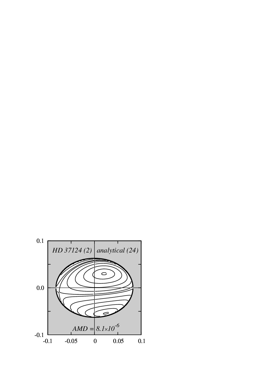


Figure 4 is for the energy levels in the symmetric representative plane computed and calculated for three slightly different orbital configurations related to possible orbital best-fits (panels in each column are for one orbital fit). Osculating elements of these configurations are quoted in the caption to this figure. The first, kinematic solution to the three-Keplerian model of the RV, is taken from the original discovery paper (Vogt et al., 2005). Other two best-fits are from Goździewski et al. (2008). The energy levels are computed for fixed calculated for each particular initial condition.
In the top row of Fig. 4 we show energy levels calculated from the octupole theory, plots in middle row are derived from the expansion of of the -order, and the bottom row illustrates the results derived from the numerical algorithm. In all cases, the analytical high-order theory is in excellent agreement with the numerical, exact theory. We checked that the magnitude of largest, relative deviations between the analytic and numerical results are of the order of . On the other hand, the octupole theory gives relatively precise insight into the structure of the phase space. All qualitative features of the energy plane are reproduced quite well.
The HD 37124 seems to be the most interesting example of the secular dynamics in the real system found in this paper. The energy planes reveal unusual dynamical structures related to the equilibria in the secular system. We know already that they can appear as extrema as well as saddle points in the representative plane. For the same , we can have three types of stationary solutions. Two of them are characterized by extrema of in the four-dimensional phase space: the first one is the maximum which appears in the quarter with , and there is the global minimum of in the quarter with and . We also found saddle points of in the quarter with , . Stationary points marked with I and II in Fig. 4 are related to extrema of , hence they are stable. By examining the eigenvalues of the linearized equations of motions in the neighborhood of the saddle point (equilibrium III), we checked out that it is linearly stable. It can be localized in the half-plane of or , depending on selected orbital parameters.
All these solutions appear in the range of moderate eccentricities, and in fact can be located close to the actual positions of the best fit solutions. The structure of the energy plane is also robust with respect to small changes of the orbital parameters. In each panel, similarly to the previous systems, we mark the energy level of the respective nominal configuration with the green thick curve. Curiously, depending on the chosen fit, the nominal system can evolve in the quarter of the representative plane characterized by librations of around (the top-right quarter), or librations of around and around (the bottom-right quarter), as well as around while can be librating around or (the top-left or the bottom-left quarter). It means, that the apses of two innermost companions can be all aligned with the apsidal line of the outermost planet, they can be also anti-aligned or the apsidal directions can be mixed.
The presence of these stationary solutions can be interpreted in terms of the two-planet theory. We recall that for the case of two planets, mode I (with apsides aligned) corresponds to the maximum of the secular energy, while mode II (apsides anti-aligned) corresponds to the minimum of . In the case of three planets, we add the secular energies of three pairs of interacting planets. Hence, in a region of the representative plane where the maxima of of these three planetary pairs can roughly coincide, we can obtain the maximum of the total energy; by adding in the region where the particular minima are close enough in the parameter space, we can obtain the global minimum of the energy, and in the case of superimposed minimum and other maximum we can obtain the saddle of the total energy. Geometrically, the equilibria can be interpreted as combinations of the secular modes known from the theory of nonresonant two-planet system. For instance, the maximum of can be related to triple mode I (i.e., the neighboring solutions are characterized with librations around for all pairs of planets), and the saddle point of is obtained for a superposition of mode I for some pair(s) and of mode II for the other pair(s). It is not clear for us yet, what would mean a combination with the NSR mode, in the regime of large eccentricities (i.e., in the region of nonlinear-secular resonance). Likely, it could be related to sophisticated secular dynamics.
4 Conclusions
The number of multi-planet extrasolar systems constantly grows. The Doppler spectroscopy remains the most effective detection technique. Unfortunately, the measurements of RV are in some sense degenerate because due to symmetry of the Doppler signal, we usually cannot determine the true inclination of planetary orbits. Other parameters are usually determined with large uncertainties. Hence, to characterize the dynamics of such systems we cannot rely only on single initial conditions and effective, qualitative methods of dynamical analysis are very desirable.
In this paper we consider the secular theory of a coplanar -planet system which is far from MMRs and orbital collision zones. In this case, the high-frequency interactions can be averaged out and we obtain greatly simplified picture of the long-term behavior of the system. This idea leads to the classic Laplace-Lagrange theory and its modern generalizations like the octupole theory (Ford et al., 2000; Lee & Peale, 2003), high-order expansion of the secular perturbation (Henrard & Libert, 2005; Rodríguez & Gallardo, 2005) or the semi-numerical averaging invented by Michtchenko & Malhotra (2004).
Our work can be considered as a generalization of the octupole theory for hierarchical triple systems characterized with large ratio of semi-major axes. We have shown that in this case the perturbation can be averaged out over mean longitudes with very basic change of integration variables that makes it possible to express the integrand function as a polynomial of trigonometric functions, without any need of relatively complex Fourier expansions. To the best of our knowledge, such method has been not applied in the literature. However, during the final preparation of the manuscript we found a book of Valtonen & Karttunen (2006), who use a similar idea to construct the octupole theory of hierarchical triple stellar systems.
Basically, the secular Hamiltonian is expressed through the power series with respect to the ratios of semi-major axes, without an explicit limitation on the eccentricities. These series can be continued to practically any order. However, if we apply the averaging algorithm presented in this work, the convergence region of these series is usually limited. To avoid this problem, in this paper we also propose a further improvement of this method and to generalize the expansion to the spatial problem. Our theory significantly improves the octupole theory of two-planet systems. We have shown that it can be generalized to any -planet system fulfilling the assumption of the averaging theorem. The simple “trick” of choosing the integration variables can be applied not only for purely gravitational point-to-point interactions but also in other models in which the mutual interactions can be expressed in powers of mutual distance between objects in the system. For instance, now we work on applying the averaging algorithm to relativistic and quadrupole moment perturbations (Migaszewski & Goździewski, 2008b). Its generalization to the 3D problem (in particular, for two-planet system) is also straightforward. Then it can be applied to the study of secular dynamics in hierarchical triple-star systems or star–planet configurations fulfilling assumptions of the secular theory.
In this work, the secular theory is used to investigate stationary solutions in the three-planet systems that are relatively frequent in the known sample of extrasolar planets. We found that the libration modes known in two-planet configurations can be generalized for the multi-planet model. Still, our study of particular systems is quite preliminary and new, yet unknown stationary solutions are expected to exist in this problem.
Acknowledgments
We thank Tatiana Michtchenko for a detailed review and corrections that improved the manuscript. This work is supported by the Polish Ministry of Sciences and Education, Grant No. 1P03D-021-29. C.M. is also supported by Nicolaus Copernicus University Grant No. 408A.
References
- Arnold et al. (1993) Arnold V. I., Kozlov V. V., Neishtadt A. I., 1993, Dynamical systems III. Mathematical aspects of classical and celestial mechanics. Encyclopaedia of mathematical sciences, Springer Verlag
- Barnes & Greenberg (2006) Barnes R., Greenberg R., 2006, ApJL, 647, L163
- Barnes & Greenberg (2008) Barnes R., Greenberg R., 2008, arXiv:astro-ph/0801.3226
- Bean et al. (2008) Bean J. L., McArthur B. E., Benedict G. F., Armstrong A., 2008, ApJ, 672, 1202
- Blaes et al. (2002) Blaes O., Lee M. H., Socrates A., 2002, ApJ, 578, 775
- Brouwer & Clemence (1961) Brouwer D., Clemence G. M., 1961, Methods of celestial mechanics. New York: Academic Press, 1961
- Brumberg (1995) Brumberg V. A., 1995, Analytical Techniques of Celestial Mechanics. Springer-Verlag
- Butler et al. (2006a) Butler R. P., Wright J. T., Marcy G. W., Fischer D. A., Vogt S. S., Tinney C. G., Jones H. R. A., Carter B. D., Johnson J. A., McCarthy C., Penny A. J., 2006a, ApJ, 646, 505
- Butler et al. (2006b) Butler R. P., Wright J. T., Marcy G. W., Fischer D. A., Vogt S. S., Tinney C. G., Jones H. R. A., Carter B. D., Johnson J. A., McCarthy C., Penny A. J., 2006b, ApJ, 646, 505
- Deprit (1969) Deprit A., 1969, Celestial Mechanics, 1, 12
- Ellis & Murray (2000) Ellis K. M., Murray C. D., 2000, Icarus, 147, 129
- Ferraz-Mello (2007) Ferraz-Mello S., ed. 2007, Canonical Perturbation Theories - Degenerate Systems and Resonance Vol. 345 of Astrophysics and Space Science Library
- Ferraz-Mello et al. (2006) Ferraz-Mello S., Micchtchenko T. A., Beaugé C., 2006, Regular motions in extra-solar planetary systems. Chaotic Worlds: from Order to Disorder in Gravitational N-Body Dynamical Systems, pp 255–+
- Fischer et al. (2008) Fischer D. A., Marcy G. W., Butler R. P., Vogt S. S., Laughlin G., Henry G. W., Abouav D., Peek K. M. G., Wright J. T., Johnson J. A., McCarthy C., Isaacson H., 2008, ApJ, 675, 790
- Ford et al. (2000) Ford E. B., Kozinsky B., Rasio F. A., 2000, ApJ, 535, 385
- Gladman (1993) Gladman B., 1993, Icarus, 106, 247
- Goździewski et al. (2008) Goździewski K., Breiter S., Borczyk W., 2008, MNRAS, 383, 989
- Goździewski et al. (2007) Goździewski K., Maciejewski A. J., Migaszewski C., 2007, ApJ, 657, 546
- Henrard & Libert (2005) Henrard J., Libert A.-S., 2005, in Knezevic Z., Milani A., eds, IAU Colloq. 197: Dynamics of Populations of Planetary Systems The secular planetary three body problem revisited. pp 49–54
- Hori (1966) Hori G., 1966, PASJ, 18, 287
- Ji et al. (2007) Ji J., Kinoshita H., Liu L., Li G., 2007, ApJ, 657, 1092
- Jones et al. (2002) Jones H. R. A., Paul Butler R., Marcy G. W., Tinney C. G., Penny A. J., McCarthy C., Carter B. D., 2002, MNRAS, 337, 1170
- Laskar & Robutel (1995) Laskar J., Robutel P., 1995, Celestial Mechanics and Dynamical Astronomy, 62, 193
- Lee & Peale (2003) Lee M. H., Peale S. J., 2003, ApJ, 592, 1201
- Libert & Henrard (2005) Libert A.-S., Henrard J., 2005, Celestial Mechanics and Dynamical Astronomy, 93, 187
- Libert & Henrard (2006) Libert A.-S., Henrard J., 2006, Icarus, 183, 186
- Lovis et al. (2006) Lovis C., Mayor M., Pepe F., Alibert Y., Benz W., Bouchy F., Correia A. C. M., Laskar J., Mordasini C., Queloz D., Santos N. C., Udry S., Bertaux J.-L., Sivan J.-P., 2006, Nature, 441, 305
- Malhotra (1993) Malhotra R., 1993, in Phillips J. A., Thorsett S. E., Kulkarni S. R., eds, Planets Around Pulsars Vol. 36 of ASPC, Orbital dynamics of PSR1257+12 and its two planetary companions. pp 89–106
- Marchal & Bozis (1982) Marchal C., Bozis G., 1982, Celestial Mechanics, 26, 311
- Michtchenko et al. (2008) Michtchenko T., Ferraz-Mello S., Beaugé C., 2008, in Dvorak R., ed., Extrasolar Planets Physics Textbook, Dynamics of Extrasolar Planatary Systems. pp 151–179
- Michtchenko et al. (2006) Michtchenko T. A., Ferraz-Mello S., Beaugé C., 2006, Icarus, 181, 555
- Michtchenko & Malhotra (2004) Michtchenko T. A., Malhotra R., 2004, Icarus, 168, 237
- Migaszewski & Goździewski (2008a) Migaszewski C., Goździewski K., 2008a, MNRAS, (in preparation)
- Migaszewski & Goździewski (2008b) Migaszewski C., Goździewski K., 2008b, MNRAS, (submitted)
- Morbidelli (2002) Morbidelli A., 2002, Modern celestial mechanics : aspects of solar system dynamics. Taylor & Francis
- Murray & Dermott (2000) Murray C. D., Dermott S. F., 2000, Solar System Dynamics. Cambridge Univ. Press
- Pauwels (1983) Pauwels T., 1983, Celestial Mechanics, 30, 229
- Pepe et al. (2007) Pepe F., Correia A. C. M., Mayor M., Tamuz O., Couetdic J., Benz W., Bertaux J.-L., Bouchy F., Laskar J., Lovis C., Naef D., Queloz D., Santos N. C., Sivan J.-P., Sosnowska D., Udry S., 2007, A&A, 462, 769
- Rodríguez & Gallardo (2005) Rodríguez A., Gallardo T., 2005, ApJ, 628, 1006
- Udry et al. (2007) Udry S., Bonfils X., Delfosse X., Forveille T., Mayor M., Perrier C., Bouchy F., Lovis C., Pepe F., Queloz D., Bertaux J.-L., 2007, A&A, 469, L43
- Valtonen & Karttunen (2006) Valtonen M., Karttunen H., 2006, The Three-Body Problem. Cambridge Univ. Press
- Veras & Armitage (2007) Veras D., Armitage P. J., 2007, ApJ, 661, 1311
- Vogt et al. (2005) Vogt S. S., Butler R. P., Marcy G. W., Fischer D. A., Henry G. W., Laughlin G., Wright J. T., Johnson J. A., 2005, ApJ, 632, 638