Comparing energy loss and $p_{\perp}$-broadening in perturbative QCD with strong coupling $\mathcal{N}=4$ SYM theory

Consider a heavy quark of mass $M$ passing through hot matter of temperature $T$. We suppose $T/M\ll 1$. Suppose at some time the heavy quark is moving at rapidity $\eta$ so that its energy is $M\cosh\eta$. We also assume, for reasons to be explained below, that $\cosh\eta\ll M^{3}/\hat{q}$ with the $\hat{q}$ the transport coefficient of the plasma.

The dominant cause of energy loss of the heavy quark is gluon radiation[4, 5, 6, 7, 8] induced by the medium, at least when $\cosh\eta\gg 1$ which is the region with which we shall be concerned. Induced gluon radiation is caused by gluons in the wavefunction of the heavy quark being freed by interaction with the medium. Suppose a gluon in the quark’s wavefunction has energy $\omega$ and transverse momentum $k_{\perp}$. Such a gluon will be radiated if $k_{\perp}\leq Q_{s}$ with $Q_{s}$ the saturation momentum of the medium corresponding to a length given by the coherence time, $t_{c}$, of the gluon. The energy loss will be dominated by gluons having $k_{\perp}$, and $\omega$, as large as possible. Thus, setting $k_{\perp}=Q_{s}$, we have

and using

gives

Gluons having $\frac{\omega}{k_{\perp}}=\frac{\omega}{Q_{s}}>\cosh\eta$ are strongly suppressed in the heavy quark wavefunction[4]. Taking $\omega=Q_{s}\cosh\eta$ will give the maximum energy and, combined with Eq. (4), gives

as the relevant saturation momentum. Now we see why it is necessary to keep $\cosh\eta\ll M^{3}/\hat{q}$, because this is the condition that $\frac{k_{\perp}^{2}}{M^{2}}=\frac{Q_{s}^{2}}{M^{2}}\ll 1$, which condition is the essential requirement separating heavy quark from light quark radiation dynamics. Now it is a straightforward task to give a parametric form of the rate of energy loss of a heavy quark passing through a plasma as

The $\alpha_{s}N_{c}$ in Eq. (6) corresponds to the number of gluons, in the relevant kinematic domain, in the quark wavefunction while $t_{c}$ corresponds to the time over which the gluon energy, $\omega$, is emitted. Using Eq. (3) gives

where, $Q_{s}$ should be evaluated using Eq. (5).

The difference between heavy and light quarks lies not in changing Eq. (7), which remains valid for light quarks, but in Eq. (5) which for light quarks energy loss becomes

with $E$ the energy of the light quark.

The problem of energy loss for heavy quarks in a $\mathcal{N}=4$ SYM plasma has been well studied[1, 2]. Using the AdS/CFT correspondence allows one to evaluate the energy loss in terms of the energy flowing toward the horizon through a string which goes from a $D7$ brane, whose position is given by the heavy quark mass, toward the horizon of the metric. The metric in the $AdS_{5}$ space can be written as

with

and where $u_{h}=\pi T$ and $T$ is the temperature of the plasma. The $D7$ brane is located at a position $u_{m}$ which is related to the heavy quark’s mass by

corresponding to a string at rest in the vacuum having length $u_{m}$, as it falls straight down from $u_{m}$ to $u=0$ in the fifth dimension. The energy density of the string is

In Eqs. (11) and (12), $\lambda$ is given by $\lambda=g_{YM}^{2}N_{c}$. In the energy loss problem one keeps the string moving at a constant rapidity $\eta$ where one imagines an external constant ”electric” field acting on the end of the string on the $D7$ brane and furnishing the force necessary to keep the string moving at constant velocity $v$ where $\cosh\eta=1/\sqrt{1-v^{2}}$. The resulting rate of energy loss, that is the rate of work done by the external electric field, is[1, 2]

where we have only consider the case $\cosh\eta\gg 1$.

We are now going to show that Eq. (13) agrees with Eq. (7) if one uses the saturation momentum appropriate to the $\mathcal{N}=4$ SYM plasma instead of Eq. (5). To get the replacement of Eq. (5) for the SYM plasma, we recall that the saturation momentum corresponding to a length $L$ of such a plasma is[9]

Using $t_{c}$ in Eq. (3) as the relevant length , just as we used for calculating the energy loss in QCD, and taking $\omega/Q_{s}=\cosh\eta$, one gets

from Eq. (14). Using Eq. (15) in Eq. (13), one arrives at

Except for the replacement of $\alpha N_{c}$ by $\sqrt{\lambda}$ Eq. (7) and Eq. (16) are the same. The replacement of $\alpha N_{c}$ by $\sqrt{\lambda}$ is to be expected and already occurs in comparing the static energy density, the electric field squared, of a heavy quark in QCD with that of a heavy quark in $\mathcal{N}=4$ SYM theory. As we show in Sec. III, this naturally leads a gluon distribution in a heavy quark to be the same in QCD and in $\mathcal{N}=4$ SYM theory except for the replacement of $\alpha N_{c}$ by $\sqrt{\lambda}$. Our picture of energy loss of a heavy quark in an infinite plasma is thus essentially identical in QCD and in $\mathcal{N}=4$ SYM. We do note, however, that we do not have control of constant factors in our description of energy loss in a $\mathcal{N}=4$ SYM plasma.

The picture of transverse momentum broadening of a high energy quark in QCD is very simple and is the same for light quarks as for heavy quarks[12, 13]. As the quark passes through the plasma, it interacts with quanta of the plasma through multiple single gluon exchange, each exchange giving a random transverse momentum to the quark, and two gluon exchanges, necessary to keep probability conservation. The formula

gives the rate of increase in the typical $p^{2}_{\perp}$ that the quark picks up in passing through the medium in terms of the transport coefficient of medium. One can also write this relation as

where $Q_{s}\left(t\right)$ is the saturation momentum of a length, $t$, of the medium where we do not distinguish between time and length intervals for our relativistic heavy quark. The result given in Eq. (17) and Eq. (18) comes completely from random multiple scattering of the quark in the medium. There is also a contribution from emission of gluons stimulated by the medium. The same gluon emissions which give the energy loss indicated in Eq. (7) naturally give a $p_{\perp}$-broadening

Eq. (19) is perhaps obvious once one writes Eq. (7) in the form

where $\omega\left(t\right)$ is given by Eq. (4) with the $t$ -dependence of $Q_{s}$ given by Eq. (2), identifying $t_{c}$ with $t$. Then Eq. (19) and Eq. (20) directly give the energy loss and transverse momentum broadening due to gluon radiation stimulated by the medium. The contribution of Eq. (19) is usually neglected because it is parametrically smaller than the contribution given in Eq. (18) from multiple scattering. However, as we shall see below in a SYM plasma, transverse momentum broadening of a heavy quark is dominated by gluon radiation because $\alpha N_{c}$ will be replaced by the large parameter, $\sqrt{\lambda}$.

The calculation of transverse momentum broadening in a SYM plasma is done in terms of fluctuations on the corresponding string on the gravity side of the AdS/CFT correspondence. The result is[14, 15]

If we identify the saturation momentum $Q_{s}$ as in Eq. (15), then one can write

or, alternatively, as

where, again, we identify $t$ with $t_{c}$ the coherence time of the gluons whose emission dominates both the energy loss and transverse momentum broadening of the heavy quark. Eq. (23) is identical, after $\alpha N_{c}\leftrightarrow\sqrt{\lambda}$, with Eq. (19) adding confirmation to our picture of energy loss and $p_{\perp}$-broadening as due to gluon emission in the SYM plasma. Once one writes formulas in terms of the relevant saturation momentum, the SYM and QCD pictures become identical. Of course, in the case of $p_{\perp}$-broadening what is a subdominant effect in QCD, gluon emission, becomes dominant in the SYM plasma.

Our picture of infinite extent plasmas has been that a heavy quark loses energy and gets transverse momentum broadening by the emission of gluons having transverse momentum equal to the saturation momentum of the medium corresponding to a medium length given by the coherence length of the emitted gluons which carry the same rapidity as the parent heavy quark. Now we are going to identify this picture more closely with the trailing string picture.

In the trailing string picture, a heavy quark moving at constant rapidity through a SYM plasma correponds to a string moving at the same rapidity in the background metric, Eq. (9) on the AdS side of the correspondence. The shape of the string is[1, 2]

where

with $M$ the mass of the heavy quark. In our picture, the parts of the string having $u_{m}>u>Q_{s}$ correspond to gluons actually in the heavy quark while those parts of the string having $u_{h}<u<Q_{s}$ correspond to freed matter which is no longer part of the heavy quark. The flow of energy past the point

with $Q_{s}$ given as in Eq. (15), corresponds to the freeing of gluons from the heavy quark and into QCD plasma. Let us now see that $u\sim u_{s}$ is a natural point on the string for separating the heavy quark from waves in the plasma. Let $\Delta z\left(u\right)$ be the distance between a point on the trailing string and a corresponding point on a string, having the same motion at $u=u_{m}$, moving in the vacuum. Using Eq. (24) for $u$ large, one easily finds

Now we expect that the range of z-values allowed in a heavy quark moving at velocity $v$ in the vacuum is given by

where the first factor on the right hand side of Eq. (28) is the infrared-ultraviolet correspondence while the second factor is due to Lorentz contraction. Those region of $u$ having $\Delta z\left(u\right)\leq\delta z\left(u\right)$ can naturally be part of the heavy quark while those region of $u$ having $\Delta z\left(u\right)>\delta z\left(u\right)$ lag too far behind the core of the heavy quark to be part of it. Comparing Eq. (27) and Eq. (28), we see that the separation point, up to constant factor of order one, is given by Eq. (26). In Sec. V, we give a more complete discussion of this issue where, instead of relying on Eq. (28), we compare the four-dimensional energy-momentum tensor for a trailing string with that of the string corresponding to a heavy quark moving in the vacuum and reach the same conclusion as above.

Another argument for Eq. (26) as the natural separation point between what belongs to the heavy quark and what has been freed into the medium comes from the calculation of transverse momentum broadening from small fluctuation on the trailing string. In the differential equation governing the small fluctuations $u=u_{s}$ is a regular singular point which corresponds to a horizon of the metric on the worldsheet of the string[14, 15]. Waves on the worldsheet of the string going from large $u$ can disappear into the horizon but one requires that waves not come out of the horizon toward large values of $u$.[22, 23]

In dealing with hot matter of finite length in QCD, the energy loss problem is very different for dressed and bare quarks. For heavy ion collisions where high transverse momentum quarks are produced in the collision as bare quarks, without the accompanying gluon cloud which characterize a dressed quark, the dressed quark energy loss problem is of little interest. Nevertheless we begin with this problem in our discussion of finite matter because it is relatively straightforward.

The situation is as follows: A high energy heavy quark prepared at early times impinges on a target of hot matter, say a cube, of length $L$. We wish to determine how much energy is lost and how much transverse momentum broadening occurs as the heavy quark passes through the medium. If the rapidity of the heavy quark is such that $\cosh\eta\ll\left(LT\right)^{2}$(For QCD the condition is $\cosh\eta\ll\sqrt{\hat{q}L^{3}}$), then the coherence time of all the gluons in the heavy quark is much less than $L$ and the matter is effectively of infinite extent. Thus, we consider here only the opposite case where $\cosh\eta\gg\left(LT\right)^{2}$. We also suppose $\frac{M}{LT^{2}}\gg 1$ so that a small fraction of the heavy quark’s energy is lost as it passes through the matter.

When $\cosh\eta\gg\left(LT\right)^{2}$, the picture is essentially the same in QCD and for a SYM plasma. Gluons in the heavy quark wavefunction having $k_{\perp}<Q_{s}\sim LT^{2}$ will be freed in passing through the matter while those having $k_{\perp}\geq Q_{s}$ are not freed. Since the gluons which dominate the energy loss have $\omega\simeq k_{\perp}\cosh\eta$, the energy loss will be

with $\alpha N_{c}$ referring to QCD and $\sqrt{\lambda}$ to the SYM case. For SYM the result Eq. (29) agrees with Eq. (13), the infinite matter result, when Eq. (14) is used for $Q_{s}$. For QCD the result Eq. (29) differs from the case of infinite matter, and we remark that we have not subtracted the ”factorization term”[24, 25]. We emphasize, however, that when written in terms of the saturation momentum the QCD and SYM results are of the same form once one makes the $\alpha N_{c}\leftrightarrow\sqrt{\lambda}$ identification in passing between theories.

For transverse momentum broadening the formulas are

where again the upper value is for QCD while the lower value is for a SYM plasma. The QCD result is the same as Eq. (17) for infinite matter while the SYM result takes the same form as infinite matter, as given in Eq. (22), but now one must use Eq. (14) for $Q_{s}^{2}$. The argumentation leading to Eq. (30) is identical to that giving Eq. (29) and, again, here in the SYM plasma transverse momentum broadening is radiation dominated.

The quarks, whether light or heavy, that are produced in hard collisions in a relativistic heavy ion collision are initially bare, that is they have been produced without the gluon cloud that accompanies a quark which is part of a high energy hadron. While the energy loss of bare quarks has been widely discussed in the QCD literature[5, 6, 7, 8], it has so far not been treated in the literature on the SYM plasma. On the string theory side of the AdS/CFT correspondence, in order to create a heavy quark which is initially bare it is necessary to consider a heavy quark-antiquark pair initially with little or no separation and then rapidly accelerate the quark and the antiquark in opposite direction by, say, an electric field $E_{f}$ which is constant in space and time and points along the $z$-axis. After a rapid acceleration over a time $t_{1}$, the electric field can be turned off and one has a quark-antiquark pair with large relative energy in a situation similar to that occurring in a hard collision[1]. We have found an exact solution which satisfies the equations coming from the Nambu-Goto action for the quark-antiquark pair accelerating in the vacuum. This will be discussed in much more detail in Sec. IV and in Ref. [17], while here we give the solution and use it to outline how to get energy loss and $p_{\perp}$-broadening in a SYM plasma.

The solution, in the vacuum, described above is

where the external electric field is

The quark is at $z>0$ and antiquark is at $z<0$. $M$ is the mass of the heavy quark as usual. The constant $c$ characterizes the strength of the electric field and $c\geq 1$ is required, as is clear from Eq. (31). We imagine $c$ to be large but we also suppose $\frac{u_{m}}{c}$ is very large compared to the temperature of the medium which we shall shortly introduce. At a time $t_{1}$, we shall turn off the electric field beyond which time Eq. (31) no longer applies. It is straightforward to see that, for $t<t_{1}$, the part of the string in the region $u_{m}/c<u<u_{m}$ moves with a rapidity $\eta\left(t\right)$ given by

We now suppose that

however, we also imagine that $t_{1}$ is a small time compared to the inverse temperature of the medium. By choosing $u_{m}$ sufficiently large there is no difficulty in having $c\gg 1$, $u_{m}t_{1}/c\gg 1$, and $t_{1}T\ll 1$ satisfied.

Before considering motion in a plasma, let us examine a little further the vacuum evolution of our heavy quark-antiquark system. When $c/u_{m}<t<t_{1}$, it is useful to consider the $z>0$ part of the string as two parts. Part A consists of the $u_{m}/c\leq u\leq u_{m}$ region of the string, while part B is the $\frac{1}{\sqrt{t^{2}+c^{2}/u_{m}^{2}}}\leq u<u_{m}/c$ region of the string. Much as in the trailing string , part A is part of the heavy quark, while part B corresponds to radiated energy. Indeed with this interpretation we can calculate the power radiated at time $t$ as

The first term on the right hand side of Eq. (35) gives the rate at which the electric field puts energy into the system. Noting that the energy density of a string at rest is $\frac{dE}{du}=\frac{\sqrt{\lambda}}{2\pi}$, we see that the second term is the rate of growth of the energy in the ”straight section” of the string in the region $u_{m}/c\leq u\leq u_{m}$. Eq. (35) gives

We note that the answer for a classical electron accelerating in a constant electric field is[26]

parametrically the same as Eq. (36) with the replacement $e^{2}\leftrightarrow\sqrt{\lambda}$.

Armed with our understanding that the part of the string $u<u_{m}/c$ is emitted radiation and no longer part of the heavy quark, we are now ready to insert the medium. We suppose that the acceleration during $0<t<t_{1}$ takes place at one end of a hot SYM plasma whose $z$-extent is $L$. At $t=t_{1}$, we turn off the electric field and let our heavy quark pass through the length $L$ of the plasma. There are two separate cases to consider: (i), when $\cosh\eta\left(t_{1}\right)\equiv\cosh\eta\ll\left(LT\right)^{2}$ and (ii), when $\cosh\eta\gg\left(LT\right)^{2}$.

In case(i), the situation is just like that of a trailing string in an infinite medium. In vacuum the separation point between that part of the string corresponding to the heavy quark and previously radiated energy is at $u=\frac{u_{m}}{c}\frac{t_{1}}{t}=\frac{\cosh\eta}{t}$ when $t>t_{1}$. At a time $t=\frac{\sqrt{\cosh\eta}}{T}$ this point crosses the separation point, $u=T\sqrt{\cosh\eta}$, of the trailing string at which point the heavy quark energy loss and transverse momentum broadening becomes that of the trailing string. This time at which the string becomes a trailing string is much less than $L$ so that the whole problem becomes that of an infinite medium trailing string problem. In case (i), $\cosh\eta$ is small enough that the system quickly adjust to the trailing string scenario.

In case(ii) the situation is much more subtle. To better appreciate the issues, let us first suppose the motion of the evolving string to take place in the vacuum. Then, when the electric field is turned off at $t=t_{1}$, the system will go toward a final configuration of a heavy quark moving in the vacuum at constant velocity along with some radiation. The radiation all goes toward $u=0$ as explained in detail in Ref. [16]. For us the key issue is at what time the quanta making up the heavy quark are formed. We know that the separation point, which is at $u=u_{m}/c$ for $t<t_{1}$, moves down in $u$ as

when $t>t_{1}$, essentially according to free branching. However, once the electric field has been turned off this separation point need no longer be a perfect separation between what is part of the heavy quark and what is radiated energy. Although almost all the energy in the region $u<\left(u\right)_{\text{separation}}$ lags too far behind the core of the heavy quark to be part of it, at a distance

behind the core as is clear from Eq. (31), the components of the heavy quark having $k_{\perp}\sim u$ and $k_{z}\sim tu^{2}\ll u\cosh\eta$ spatially overlap with the evolving string as is evident in the discussion in Sec. V and on Fig.1. If these components of the evolving string do contribute to the final heavy quark, they are formed at a time $t_{c}$ where

which matches our expectation of the time at which such components are naturally formed. Of course the components of the heavy quark carrying most of the energy, having $k_{z}\simeq u\cosh\eta$, would still be formed much later at the time when the separation point, given in Eq. (38), reaches u.

It is the identification of $\frac{k_{z}}{k_{\perp}^{2}}\simeq\frac{k_{z}}{u^{2}}$ with the time at which soft components, those where $\frac{k_{z}}{u\cosh\eta}\ll 1$, of the free heavy quark are formed which drives us toward identifying a (small) part of the evolving string having $u<\left(u\right)_{\text{separation}}$ as contributing to the heavy quark. We now make this conjecture, namely that after the electric field has been turned off at $t=t_{1}$, the parts of the heavy quark having $k_{\perp}\sim u$ and $k_{z}$ are formed at a time $t_{c}\sim k_{z}/u^{2}$ out of a small fraction, a fraction $\frac{k_{z}}{u\cosh\eta}$, of the energy of the evolving string located at $u$ at time on the order of $t_{c}$.

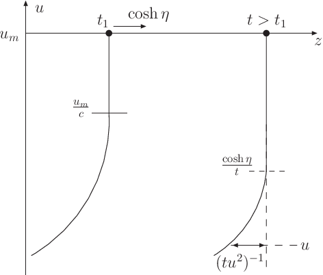
Now let us return to the string evolving in the SYM medium. After the electric field is turned off, the system goes toward radiation and a partially formed heavy quark passing through the medium. In our present situation, $\cosh\eta\gg\left(LT\right)^{2}$, the heavy quark is only fully formed after leaving the medium. Now medium induced energy loss is determined by which components of the heavy quark which are forming in the medium are inhibited from doing so by the medium. Clearly all momentum components $k_{\perp}\sim u<Q_{s}$ will be inhibited. Thus the energy loss will be equal to that part of the free heavy quark string having $u<Q_{s}$ and $\frac{k_{z}}{u^{2}}<L$, or

exactly as in Eq. (16), but where now

Similarly the transverse momentum broadening is given as

as in Eq. (23) but now with Eq. (42) again determining $Q_{s}$.

The rather elaborate argument we have just given for energy loss, and which also give Eq. (42) for $p_{\perp}$-broadening is essentially identical to the understanding of energy loss in perturbative QCD in a finite length medium[5, 6, 7, 8, 13, 18]. So it should be no surprise that there the result is

and

when $\cosh\eta>\sqrt{\hat{q}L^{3}}$ and where the $Q_{s}^{2}$ in Eqs. (44) and (45) is given by $Q_{s}^{2}=\hat{q}L$.

We set up our accelerating string calculation as follows: a quark-antiquark pair is imbedded in a brane located at $u=u_{m}$, and a net electric field $E_{f}$ is imposed in the brane which accelerates the quark and antiquark at a constant acceleration in their own proper frame (An additional small electric field $E_{f2}$ which balances the attractive force between the quark and antiquark is also understood.).

The metric of the resulting vacuum $Ad_{5}$ space can be written as

where $R$ is the curvature radius of the $AdS_{5}$ space and $\bar{u}=\frac{1}{u}$. The dynamics of a classical string is characterized by the Nambo-Goto action,

where $\left(\tau,\sigma\right)$ are the string world-sheet coordinates, and $-\det g_{ab}=-g$ is the determinant of the induced metric. $T_{0}$ is the string tension. We define $X^{\mu}\left(\tau,\sigma\right)$ as a map from the string world-sheet to the five dimensional space time, and introduce the following notation for derivatives: $\dot{X}^{\mu}=\partial_{\tau}X^{\mu}$ and $X^{\prime\mu}=\partial_{\sigma}X^{\mu}$. When one chooses a static gauge by setting $\left(\tau,\sigma\right)=\left(t,u\right)$, and defines $X^{\mu}=\left(t,u,x\left(t,u\right),0,0\right)$, it is straightforward to find that

Therefore, the equation of motion of the classical string reads:

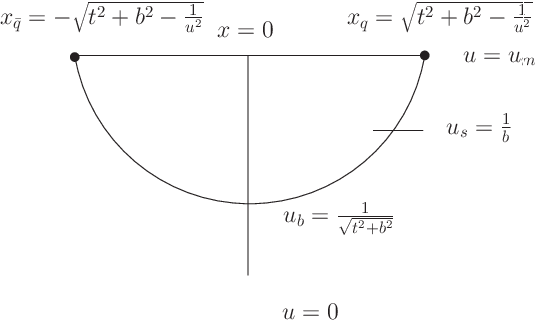
In general, this equation is a non-linear differential equation which involves two variables and two derivatives. Thus it is notoriously hard to solve directly when $x\left(t,u\right)$ is a non-trivial function of $\left(t,u\right)$. Fortunately, we have been able to find an exact solution which corresponds to the accelerating string. The solution reads,

where the $+$ part represents the right moving part of the string and the $-$ part yields the left moving part of the string, together with the smooth connection in the middle (see Fig. 2). The quark and antiquark are accelerating and moving away from each other. The constant $b$ can be fixed by the boundary condition, and corresponds to $b=\frac{c}{u_{m}}$ from Sec. II, where $c$ is a dimensionless quantity. It is very easy to check that Eq. (66) satisfies the equation of motion by noting that $\sqrt{-g/R^{4}}=\frac{b}{\sqrt{t^{2}+b^{2}-\frac{1}{u^{2}}}}$.

Following Herzog et al [1] , one can compute the canonical momentum densities associated with the accelerating string,

The energy density is given by $\pi_{t}^{0}$,

Thus the total energy of the right half string at time $t$ is,

Moreover, the energy flow is given by $\pi_{t}^{1}$,

Thus the net energy¹¹ 1 The total energy being put into the system should be the sum of the work done by $E_{f}$ and $E_{f2}$. $E_{f}$ is the field giving constant acceleration in the absense of Coulomb attraction between the heavy quark and antiquark. The field $E_{f2}$ is included to cancel that Coulomb force and is therefore time dependent. However only $E_{f}$ contributes to the non-Coulomb net energy increase and to the constant acceleration $E_{f}/M$. being put into the right half string from $0$ to $t$ is,

with the second term in the bracket being the initial energy deposited in the string. Also $b^{2}-\frac{1}{u_{m}^{2}}\geq 0$ is assumed for consistency. Therefore, from energy conservation, one can easily fix the constant $b$ by setting $E_{f}=\frac{T_{0}R^{2}u_{m}}{b}$, then,

where $M=T_{0}R^{2}u_{m}$ is the mass of the heavy quark and $T_{0}R^{2}=\frac{\sqrt{\lambda}}{2\pi}$ according to the AdS/CFT correspondence. It is now very easy to see the physical interpretation of the constant $b$ as the reciprocal of the constant acceleration $a$, i.e., $a=\frac{E_{f}}{M}=\frac{1}{b}$.

In addition, although $\frac{\partial x}{\partial t}=\frac{t}{\sqrt{t^{2}+b^{2}-\frac{1}{u^{2}}}}$ exceeds $1$ when $u$ becomes smaller than $1/b$, one can compute the speed at which energy travels by the following,

and find that $v\leq 1$ at all times. In arriving at the above result, one needs to look at the hypersurface where energy is constant. Then, one can also obtain $\frac{du}{dt}=-\frac{\partial E}{\partial t}/\frac{\partial E}{\partial u}=-\frac{ut}{t^{2}+b^{2}}$. Finally, the Lorentz boost factor of the string reads,

and it reduces to $\frac{t}{b}=\frac{tu_{m}}{c}$ in the large $t$ and $u$ limits.

In a following paper[17], we will explicitly show that there is a scale $u_{s}=\frac{1}{b}$ separating the soft part(the lower part) of the string from the hard part of the string(the upper part). The upper part, which moves together with the heavy quark, corresponds to the co-moving hard partons in the heavy quark wave function; The lower part ($u<u_{s}$) of the string, which lies far behind the heavy quark, is emitted radiation, and it is no longer part of the heavy quark.

Therefore, the radiated energy at time $t$ is

and the radiation power reads,

in agreement with Eq. (35). By using the same picture, we can also estimate the $p_{T}$ and $p_{L}$ broadening due to radiation. At large time limit, one finds

where $\sqrt{\lambda}$ basically counts the number of partons being emitted, $u_{s}^{2}$ is the typical momentum square of the emitted partons, and $t$ is just the time scale of the system. Similarly, one finds

with $\omega_{s}\sim\frac{1}{\Delta x}\simeq u_{s}^{2}t$ being the typical energy of the emitted partons and $\Delta x$ being the longitudinal separation between the quark and the string at $u=u_{s}$. Moreover, after identifying $u_{s}$ with $Q_{s}$, one discovers that the coherence time $t=\frac{\omega}{u_{s}^{2}}$ in this accelerating string scenario coincides with the one in QCD (see Eq. (3)).

The exact evaluation by employing random fluctuation analysis will be provided in Ref. [17], and it yields

Finally, we have checked that our solution Eq. (77) gives the same radiation as that of Mikhailov’s general radiation formulas[27] when specialized to the case of constant acceleration.

The metric of the resulting AdS black brane solution in 5 dimension with finite temperature $T$ can be written as

References

- [1] C. P. Herzog, A. Karch, P. Kovtun, C. Kozcaz and L. G. Yaffe, JHEP 0607, 013 (2006).
- [2] S. S. Gubser, Phys. Rev. D 74, 126005 (2006) [arXiv:hep-th/0605182].
- [3] H. Liu, K. Rajagopal and U. A. Wiedemann, Phys. Rev. Lett. 97, 182301 (2006) [arXiv:hep-ph/0605178].
- [4] Y. L. Dokshitzer and D. E. Kharzeev, Phys. Lett. B 519, 199 (2001) [arXiv:hep-ph/0106202].
- [5] R. Baier, Y. L. Dokshitzer, A. H. Mueller and D. Schiff, Nucl. Phys. B 531, 403 (1998) [arXiv:hep-ph/9804212].
- [6] B. G. Zakharov, JETP Lett. 63, 952 (1996) [arXiv:hep-ph/9607440]; JETP Lett. 65, 615 (1997) [arXiv:hep-ph/9704255].
- [7] M. Gyulassy, P. Levai and I. Vitev, Phys. Rev. Lett. 85, 5535 (2000) [arXiv:nucl-th/0005032];Nucl. Phys. B 594, 371 (2001) [arXiv:nucl-th/0006010].
- [8] C. A. Salgado and U. A. Wiedemann, Phys. Rev. D 68, 014008 (2003) [arXiv:hep-ph/0302184].
- [9] Y. Hatta, E. Iancu and A. H. Mueller, JHEP 0801, 063 (2008) [arXiv:0710.5297 [hep-th]].
- [10] P. M. Chesler and L. G. Yaffe, Phys. Rev. Lett. 99, 152001 (2007). [arXiv:0706.0368 [hep-th]]; arXiv:0712.0050 [hep-th] .
- [11] S. S. Gubser and S. S. Pufu, Nucl. Phys. B 790, 42 (2008).
- [12] G. T. Bodwin, S. J. Brodsky and G. P. Lepage, Phys. Rev. Lett. 47, 1799 (1981).
- [13] R. Baier, Y. L. Dokshitzer, A. H. Mueller, S. Peigne and D. Schiff, Nucl. Phys. B 484, 265 (1997) [arXiv:hep-ph/9608322].
- [14] S. S. Gubser, Nucl. Phys. B 790, 175 (2008) [arXiv:hep-th/0612143].
- [15] J. Casalderrey-Solana and D. Teaney, JHEP 0704, 039 (2007) [arXiv:hep-th/0701123];Phys. Rev. D 74, 085012 (2006) [arXiv:hep-ph/0605199].
- [16] Y. Hatta, E. Iancu and A. H. Mueller, arXiv:0803.2481 [hep-th].
- [17] B. W. Xiao, arXiv:0804.1343 [hep-th].
- [18] R. Baier, Y. L. Dokshitzer, A. H. Mueller, S. Peigne and D. Schiff, Nucl. Phys. B 483, 291 (1997) [arXiv:hep-ph/9607355].
- [19] J. M. Maldacena, Adv. Theor. Math. Phys. 2, 231 (1998) [Int. J. Theor. Phys. 38, 1113 (1999)] [arXiv:hep-th/9711200].
- [20] E. Witten, Adv. Theor. Math. Phys. 2, 253 (1998) [arXiv:hep-th/9802150].
- [21] S. S. Gubser, I. R. Klebanov and A. M. Polyakov, Phys. Lett. B 428, 105 (1998) [arXiv:hep-th/9802109].
- [22] C. P. Herzog and D. T. Son, JHEP 0303, 046 (2003) [arXiv:hep-th/0212072].
- [23] D. T. Son and A. O. Starinets, Ann. Rev. Nucl. Part. Sci. 57, 95 (2007) [arXiv:0704.0240 [hep-th]].
- [24] M. Gyulassy and X. N. Wang, Nucl. Phys. B 420, 583 (1994) [arXiv:nucl-th/9306003].
- [25] R. Baier, Y. L. Dokshitzer, S. Peigne and D. Schiff, Phys. Lett. B 345, 277 (1995) [arXiv:hep-ph/9411409].
- [26] J.D. Jackson, ”Classical Electrodynamics” 2nd edition, John Wiley and Sons, New York (1975). See especially Eq.(14.28).
- [27] A. Mikhailov, arXiv:hep-th/0305196.
- [28] A. Yarom, Phys. Rev. D 75, 105023 (2007) [arXiv:hep-th/0703095].