Quantal time asymmetry: mathematical foundation and physical interpretation

Time Asymmetry does not mean time reversal non-invariance, i.e. it is not described by a Hamiltonian $H$ that does not commute with the time reversal $A_{T}$ or the $CP$ operator [1]:

It may be intriguing, however, to speculate about a possible connection [2].

Time Asymmetry does not mean irreversibility or Thermodynamic Arrow of Time. It is not entropy increase in an isolated classical system, $\frac{dS}{dt}>0$. There may, however, be some relation to entropy increase. For instance, Peierls (1979) explains entropy increase from initial boundary conditions in Boltzmann’s Stosszahl Ansatz [3].

Time Asymmetry also does not mean the usual quantum mechanical Arrow of Time for “open” quantum systems, brought about by an external reservoir [4] described by the Liouville equation,

in which a “superoperator,” $\mathcal{I}$, describes the external effect of the reservoir, or of a measurement apparatus, or of another environment (decoherence).

By Time Asymmetry, we mean time asymmetric boundary conditions for time symmetric dynamical equations.

The best known example is the Radiation Arrow of Time [5]. Maxwell’s equations (dynamical differential equations) are symmetric in time. A boundary condition excludes the strictly incoming fields and selects only the retarded fields of the other sources in the region:

The boundary condition is an additional “principle of nature” that chooses of the two solutions of the Maxwell equations,

the retarded solution

The “disturbance” $A^{\mu}(x)$ at the position $\vec{x}$ at time $t$ is caused by the source $j^{\mu}$ at another point $\vec{x^{\prime}}$, at an earlier time $t^{\prime}=t-\frac{|\vec{x}-\vec{x^{\prime}}|}{c}\leq t$. Radiation must be emitted (at $t^{\prime}$) by a source before it can be detected by a receiver at $t\geq t^{\prime}$.

Standard quantum mechanics lacks time asymmetric boundary conditions. The dynamical equations are
  In the Heisenberg picture $\displaystyle i\hbar\frac{\partial\Lambda(t)}{\partial t}=-[H,\Lambda(t)]$ (7a) $\displaystyle i\hbar\frac{\partial}{\partial t}\psi(t)=-H\psi(t)$ (7b) for the observable $\Lambda(t)=\mid\!\!\psi(t)\rangle\langle\psi(t)\!\mid$, with state $W=\mid\!\!\phi\rangle\langle\phi\!\mid$ kept fixed.     or      In the Schrödinger picture $\displaystyle i\hbar\frac{\partial W(t)}{\partial t}=[H,W(t)]$ (8a) $\displaystyle i\hbar\frac{\partial}{\partial t}\phi(t)=H\phi(t)$ (8b) for the state $W(t)$ or $\phi(t)$ with observable $\Lambda=\mid\!\!\psi\rangle\langle\psi\!\mid$ kept fixed

In standard quantum mechanics [6], one solves these equations under the boundary conditions

The sets of operators

and

form a group, because the products $U(t_{1})U(t_{2})=U(t_{1}+t_{2})$ and the inverses $U^{-1}(t)=U(-t)$ exist. For every observable $\psi(t)=U(t)\psi$ at time $t$ there is also an observable $\psi(-t)=U^{-1}(t)\psi$ at time $-t$. The same applies for the state $\phi$ and the operator $U^{\dagger}(t)$.

In quantum physics one distinguishes [8] between states, which are described by density operators $W$ or by state vectors $\phi$, and observables, which are described by operators $A=A^{\dagger}$, $\Lambda=\Lambda^{2}$, or by observable vectors $\psi$ if $\Lambda=|\psi\rangle\langle\psi|$.
State $W$ (in-states $\phi^{+}$ of scattering experiment.) is prepared by a preparation apparatus (e.g. accelerator)
Observable $A$ (out-observables $\psi^{-}$, “out-state”) is registered by a registration apparatus (e.g. detector)
Experimental quantities, $\mathcal{P}_{W}(\Lambda(t))$, are the probabilities to measure the observable $\Lambda$ in the state $W$. They are calculated in theory as Born Probabilities. They are measured as ratios of large numbers of detector counts (“relative frequencies”).

The comparison between theory and experiment is given by

The left hand side is the calculated prediction, and the right hand side is the ratio of detector counts, where $N(t)$ and $N$ are “large” integers. The comparison between theory and experiment is indicated by $\approx$.

What is the experimental evidence for this time evolution group? It is obvious that a state $\phi$ must be prepared before the observable $\mid\!\!\psi(t)\rangle\langle\psi(t)\!\mid$ can be measured in it (causality), e.g. the detector cannot register the decay products before the decaying state has been prepared. This means that we have a Quantum Mechanical Arrow of Time:

The Born probability to measure the observable $\mid\!\!\psi(t)\rangle\langle\psi(t)\!\mid$ in the state $\phi$,

exists (experimentally) only for $t\geq t_{0}(=0)$,
where $t_{0}$ is the preparation time of the state $\phi$. In contrast, the unitary group of the Hilbert space axiom predicts $|\langle\psi(t)\!\mid\!\!\phi\rangle|^{2}$ for all $-\infty<t<+\infty$.

As a consequence of this obvious phenomenological condition (causality), one obtains the Quantum Mechanical Arrow of Time:
In the Heisenberg picture the time translated observables

In the Schrödinger picture the time evolved states

The time evolution is asymmetric, $0\leq t<\infty$, and given by the semigroup

or by the semigroup

Therefore we have the task: Find a theory (for instance choosing new boundary conditions to replace the Hilbert space axiom) for which the solutions of the Schrödinger equation are given by the semigroup $\mathcal{U}^{\times}(t)$ (20), and for which the solutions of the Heisenberg equation are given by the semigroup $\mathcal{U}(t)$ (21).

In standard quantum mechanics, time evolution is a subgroup of the space-time symmetry transformations, which, according to the Wigner-Bargmann theorem, are represented by the (projective) unitary representations in $\mathcal{H}$ of the Galilei group $G$ (for non-relativistic space-time) and the Poincare group $\mathcal{P}$ (for relativistic space-time) [9].

In the RHS formulation [10, 11, 12] using the Schwartz space Gelfand triplet, $\Phi\subset\mathcal{H}\subset{\Phi^{\times}}$, with the Dirac basis vector expansion

symmetry transformations $g\in G$ are represented by a triplet of operators [12, 13, 14]
acting on e.g. for time translations $\displaystyle U_{\Phi}(g^{-1})\subset$ $\displaystyle U(g^{-1})=U^{\dagger}(g)$ $\displaystyle\subset U^{\times}(g)$ $\displaystyle\Phi\subset$ $\displaystyle\mathcal{H}\quad\mathcal{H}$ $\displaystyle\subset\Phi^{\times}$ $\displaystyle e^{-iHt}|_{\Phi}\subset$ $\displaystyle e^{-iHt}=(e^{iHt})^{\dagger}$ $\displaystyle\subset e^{-iH^{\times}t},\quad-\infty<t<\infty.$
Here $U(g)$ is a unitary representation of $g$ in $\mathcal{H}$. $U_{\Phi}(g^{-1})$ is the restriction of $U(g^{-1})$ to the dense subspace $\Phi\subset\mathcal{H}$, which is a continuous operator with respect to the $\Phi$ topology, and $U^{\times}(g)$ is the conjugate operator of $U_{\Phi}(g^{-1})$ in $\Phi^{\times}$, defined by

The algebra of observables $H$, $J_{i}$, $P_{i}$, etc is obtained by deriving $U(g)$ using the limits with respect to the $\Phi$-topology; they are continuous operators in $\Phi$. Their conjugate operators $H^{\times}$, $J_{i}^{\times}$, etc are continuous in $\Phi^{\times}$ [13, 15].

This is a beautiful theory [10, 12, 13, 14], but it assumes that for every transformation $g\in G$ of the observable relative to the state, $g:\psi\rightarrow\psi^{g}$, there exists an inverse transformation also of the observable relative to the state (not the state relative to the observable), $g^{-1}:\psi\rightarrow\psi^{g^{-1}}$. For rotations and boosts this is meaningful, but for time translation, it would give an answer to the question: what was the probability of an observable $\psi$ in a state at a time $t_{0}+t$, with $t<0$, before the state will be prepared at $t_{0}$? This contradicts causality. Therefore one must find a space $\Phi_{+}$ for the observables $\{\psi\}$ such that the Galilei transformations of non-relativistic space-time are represented by a semigroup $U_{+}(R,t,\textbf{x},\textbf{v}),\quad t\geq 0$. Similarly, for the relativistic case mentioned in Section 8, one must find a space (which we will also call $\Phi_{+}$) in which the transformations of the detected observables relative to the prepared state form only a semigroup into the forward light cone [16] expressing Einstein causality.

To find the theory that provides the Time Asymmetry semigroup, we use scattering, resonance and decay phenomena [17]. Resonances and decaying states are characterized by definite values of the discrete quantum numbers such as charges (particles species label) and by angular momentum $j$. In addition they are defined by two real numbers. Resonances are characterized by energy $E_{R}$ and width $\Gamma$, and decaying states are characterized by energy $E_{D}$ and lifetime $\tau$. Their properties are contrasted as follows:
$(E_{R},\Gamma)$ defined by $(E_{D},R=\frac{1}{\tau})$ defined by
Breit-Wigner (Lorentzian) scattering amplitude.   exponential partial decay rate
$a_{j}^{BW}=\frac{r_{\eta}}{E-(E_{R}-i\frac{\Gamma}{2})}$; $0\leq E<\infty$ $R_{\eta}(t)=\frac{d}{dt}P_{\eta}(t)$, $R=\sum_{\eta}R_{\eta}(0)$
  $R_{\eta}(t)=R_{\eta}(0)\text{e}^{-t/\tau}=R_{\eta}(0)\text{e}^{-Rt}$
  where probability $P_{\eta}(t)=|\langle\psi_{\eta}\!\mid\!\!\phi_{D}(t)\rangle|^{2}$

Resonances appear in Decaying states are
scattering, e.g. observed in decay, e.g.
$e^{+}\,e^{-}\rightarrow Z\rightarrow e^{+}\,e^{-}$

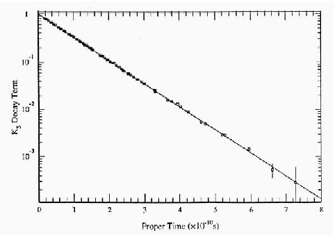
Many people think that

and especially for non relativistic quantum mechanics, a common assumption is that

This relation is based on the Weisskopf-Wigner (WW) approximation [20], and in standard quantum theory there is no proof of it, as e.g. stated by

M. Levy: [21] “…There does not exist… a rigorous theory to which these various (WW) methods can be considered as approximations.”

The energy of a resonance is the complex number
$z_{R}=E_{R}-i\frac{\Gamma}{2}$, the pole position of the $S$ matrix or of the scattering amplitude $a_{j}(E)$.

What one can show using the Weisskopf-Wigner approximation methods, is that the probability of a prepared resonance state $\phi$ with Breit-Wigner energy distribution of width $\Gamma$ is obtained as [22]

Thus, in the Weisskopf-Wigner approximation, the probability rate has a non-exponential term proportional to the width $\Gamma$. In general one can prove that there is no Hilbert space vector $\phi(t)$ that obeys the exact exponential law [23]. If, as in Figure 2 for the $K_{S}^{0}$-decay experiment, the time dependence of $\mid\!\!\langle\psi_{\pi\pi}\!\mid\!\!\phi^{K^{0}_{S}}(t)\rangle\!\!\mid^{2}=\frac{N(t_{i})}{N}$ is to be a perfect exponential (as shown by this experiment [19]) then the decaying state vector $\phi^{K^{0}_{S}}$ cannot be a Hilbert space vector.

The simplest way to derive an exactly exponential decay probability is to postulate a state vector $\phi^{G}$, which has the property

and whose decay probability into any observable $\mid\!\!\psi\rangle\langle\psi\!\mid$ is

This vector $\phi^{G}$ of Gamow [24] makes no sense in standard quantum mechanics because:

1. 1.

   It has a complex eigenvalue for a selfadjoint $H$; $\phi^{G}=\mid\!\!E_{R}-i\Gamma/2\rangle$

2. 2.

   It leads to the “exponential catastrophe” [25], because in standard quantum mechanics the time extends from $-\infty$: $-\infty<t<\infty$.

To define a vector with the properties (28)–(29), one needs a theory for which

1. 1.

   the energy extends to values in the complex plane

2. 2.

   the time is restricted to $0\leq t<+\infty$ (because a $K^{0}_{S}$ must be prepared first before one can detect its decay products $\pi^{+}\,\pi^{-}$, and to avoid the exponential catastrophe).

In the standard (Hilbert space) theory of quantum physics, the time $t$ has the values $-\infty<t<+\infty$, and the energy $E$ is real (spectrum of self adjoint Hamiltonian $H$) and bounded from below (stability of matter): $-\infty\neq E_{0}\leq E<\infty$.

Nevertheless, one speaks of complex energy:
   (i) for the analytic $S$ matrix   $S_{j}(E)\rightarrow S_{j}(z)$
   (ii) for the Gamow states   $z_{R}=E_{R}-i\Gamma/2$
   (iii) for the Lippmann-Schwinger equation
or in the propagator of field theory   $z=E\pm i\epsilon$, $\epsilon$ infinitesimal

Thus experiments require a quantum theory in which

1. 1.

   the time $t$ has a “preferred direction”: $t_{0}=0\leq t<\infty$

2. 2.

   the energy $E$ can take complex (discrete and continuous) values in the complex planes: $E\rightarrow z\in\mathbb{C_{\pm}}$.

The conclusion from this is that one has to restrict the set of allowed energy wave functions $\phi(E)=\langle^{+}E\!\mid\!\!\phi^{+}\rangle$, which in standard quantum theory in $\mathcal{H}$ are represented by a class of Lebesgue square integrable functions, to a smaller set.

The first step in this direction was already taken by Schwartz, inspired by the Dirac bra-ket formalism, when he restricted the set of classes of Lebesgue square integrable functions $\mathcal{L}^{2}=\{\{h(E)\}\}$ to the set of smooth, rapidly decreasing (Schwartz) functions $\{\phi(E)\}$. This replacement of the Hilbert space $\mathcal{H}$ by the Schwartz space $\Phi$ gave a mathematical meaning to the Dirac formalism [26].

The second step is to restrict the set of Schwartz space functions $\phi(E)$ further to the set of smooth functions that have analytic extensions in the upper and lower complex energy semiplanes, $\mathbb{C}_{+}$ and $\mathbb{C}_{-}$, respectively.

The mathematical basis for these modifications (31) are Rigged Hilbert Spaces (RHS), or Gel’fand Triplets. The RHS was not devised for Time Asymmetry or the theory of resonances and decay, but to provide a mathematical justification for Dirac’s bra- and ket-formalism [26].

Step 1 away from the Hilbert space was to get the Dirac formalism, which has the following two properties:

1. 1.

   The solutions of both the Heisenberg and the Schrödinger equations (for observables and states) have a Dirac basis vector expansion,

   $$\phi=\sum_{j,j_{3}}\sum_{n}|E_{n},j,j_{3})(E_{n},j,j_{3}\mid\!\!\phi\rangle+\sum_{j,j_{3},\eta}\int dE\,\,\mid\!\!E,j,j_{3},\eta\rangle\langle E,j,j_{3},\eta\!\mid\!\!\phi\rangle,$$

   (32)

   which is the analogue of $\vec{x}=\sum_{i=1}^{3}\vec{e}_{i}x^{i}$, and where the basis vectors $\mid\!\!E,j,j_{3},\eta\rangle\equiv\mid\!\!E\rangle$ are “eigenkets” of $H$ (and of a complete system of commuting observables for the other quantum numbers $j$, $j_{3}$, $\eta$). The basis vectors in (32) are defined as¹¹ 1 The first equality defines the conjugate operator $H^{\times}$ of $H$, $H^{\times}\supset H^{\dagger}$. the eigenkets of an operator $H$

   	$\displaystyle\langle H\phi\!\mid\!\!E,j,j_{3},\eta\rangle=\langle\phi\!\mid H^{\times}\mid\!\!E,j,j_{3},\eta\rangle$	$\displaystyle=E\langle\phi\!\mid\!\!E,j,j_{3},\eta\rangle\,\mbox{for all $\phi\in\Phi$},$		(33a)
   or as ordinary eigenvectors
   	$\displaystyle H\,|E_{n},j,j_{3},\eta)$	$\displaystyle=E_{n}\,|E_{n},j,j_{3}\eta).$		(33b)

   In (32) and (33a), the values of $E$ are from a continuous set, e.g. $0\leq E<\infty$.

2. 2.

   The co-ordinates or “scalar products” or the bra-kets $\langle E\!\mid\!\!\phi\rangle=\phi(E)$ are smooth, rapidly decreasing functions of $E$ (“Schwartz function” $\mathcal{S}_{\mathbb{R_{+}}}$). One gets

   		$\displaystyle\mbox{a Triplet of function spaces}\qquad\{\phi(E)\}=\{\psi(E)\}=\mathcal{S}_{\mathbb{R_{+}}}\subset L^{2}\subset\mathcal{S}^{\times}$		(34)
   		and corresponding to this
   		$\displaystyle\mbox{a Triplet of abstract vector spaces}\qquad\{\phi\}=\{\psi\}=\Phi\subset\mathcal{H}\subset\Phi^{\times}\ni\mid\!\!E\rangle$		(35)

   The space $\Phi^{\times}$ denotes the space of continuous antilinear functionals of the space $\Phi$; for the Hilbert space, $\mathcal{H}^{\times}=\mathcal{H}$. Dirac kets are antilinear continuous Schwartz space functionals.

The triplets (34) and (35) constitute Rigged Hilbert Spaces. ($\Phi$ has a locally convex nuclear topology such that the Dirac basis vector expansion (32) is the nuclear spectral theorem.) The RHS (34) of functions and distributions is equivalent (algebraically and topologically) to the abstract RHS (35).

This Schwartz space triplet (of axiomatic quantum field theory) will not provide Time Asymmetry, because solutions of the dynamical (Schrödinger or Heisenberg) equation with boundary condition $\phi\in\Phi$, $\psi\in\Phi$ (Schwartz space) are again given by a group [15]

$$\phi(t)=e^{-iHt}\phi(0),\quad\psi(t)=e^{iHt}\psi(0),\quad-\infty<t<+\infty.$$

(36)

For the Schwartz-Dirac kets one thus also obtains [15]

$$e^{-iH^{\times}t}\mid\!\!E\rangle=e^{-iEt}\mid\!\!E\rangle\quad-\infty<t<+\infty.$$

(37)

This means Step 1 away from the Hilbert space provides the Dirac kets (33a) and the Dirac basis vector expansion (32), but the Dirac formalism still does not lead to complex energy eigenvalues and resonance states (28),(29).

Step 2:
Because observables $\mid\!\!\psi^{-}\rangle\langle\psi^{-}\!\mid$ defined by the detector and states $\phi^{+}$ defined by the preparation apparatus are physically different entities, one should also distinguish mathematically between a space of observables, which we call $\Phi_{+}$,

$$\Phi_{+}\ni\psi^{-}=\sum_{j,j_{3},\eta}\int_{0}^{\infty}dE\,\mid\!\!E,j,j_{3},\eta^{-}\rangle\langle^{-}E,j,j_{3},\eta\!\mid\!\!\psi^{-}\rangle\\$$

(38)

and a space of states, which we call $\Phi_{-}$

$$\Phi_{-}\ni\phi^{+}=\sum_{j,j_{3},\eta}\int_{0}^{\infty}dE\,\mid\!\!E,j,j_{3},\eta^{+}\rangle\langle^{+}E,j,j_{3},\eta\!\mid\!\!\phi^{+}\rangle\,.$$

(39)

The two Dirac basis vector expansions (38), (39) use different kinds of Dirac kets, which we denoted:

$$\mid\!\!E,j,j_{3},\eta^{\mp}\rangle\in\Phi^{\times}_{\pm}.$$

(40)

This is suggested by the Lippmann-Schwinger in-plane waves $\mid\!\!E^{+}\rangle$ for the prepared in-states $\phi^{+}$, and the Lippmann-Schwinger out-plane waves $\mid\!\!E^{-}\rangle$ for the detected out-observables $\psi^{-}.$²² 2 The only major alteration of the Standard S-matrix formalism is that here we use out-observables fulfilling the Heisenberg equation, and not out-states fulfilling the Schrödinger equation.

Because of the $+i\epsilon$ in the Lippmann-Schwinger equation, the energy wave function of the prepared in-state $\phi^{+}$,

$$\phi^{+}(E)=\langle^{+}E,j,j_{3},\eta\!\mid\!\!\phi^{+}\rangle=\overline{\langle\phi^{+}\!\mid\!\!E,j,j_{3},\eta^{+}\rangle},$$

(41)

is the boundary value of an analytic function in the lower complex energy semi-plane (for complex energy $z=\overline{E+i\epsilon}=E-i\epsilon$ immediately below the real axis 2nd sheet of the S-matrix $S_{j}(z)$). Similarly, one surmises that the energy wave function of the observable $\mid\!\!\psi^{-}\rangle\langle\psi^{-}\!\mid,$

$$\psi^{-}(E)\equiv\langle^{-}E,j,j_{3},\eta\!\mid\!\!\psi^{-}\rangle,$$

(42)

extends to an analytic function in the upper complex energy plane. Thus one conjectures that energy wave functions can only be those Schwartz functions that can be analytically continued into the lower or upper complex energy semiplane, respectively. The space of allowed state vectors must be smaller than the Schwartz space, and the space of allowed kets will be larger than the set of Dirac kets and thus can include the eigenkets of complex energy.

To conjecture the spaces of $\phi^{+}$ and of $\psi^{-}$, we start with the definition of a resonance by an S-matrix pole at $z_{R}=E_{R}-i\Gamma/2$. If we derive from it

which has the properties:
1. it is an eigenket with a discrete complex eigenvalue (as Gamow wanted) of the Hamiltonian:

and 2. it has the time evolution

then we will have shown that:

and we will have a theory that unites resonance scattering and exponential decay.

To derive these results, further conditions had to be put on the analytic wave functions $\phi^{+}(z)$ and $\overline{\psi^{-}(z)}$ in the lower complex semiplane second sheet. These conditions suggested Hardy functions (H. Baumgartel).

Thus one is led to a new hypothesis [17]:
The energy wave functions of a state are smooth Hardy functions analytic on the lower complex semiplane $\mathbb{C}_{-}$:

The energy wave functions of an observable are smooth Hardy functions analytic on the upper complex semiplane $\mathbb{C}_{+}$:

This hypothesis is not so far off from the properties that one often used for mathematical manipulations in scattering theory. This new hypothesis led to the construction of the two Hardy space triplets [27], i.e. two RHS’s from which the two Dirac basis vector expansions (38),(39) follow as the nuclear spectral theorem [28].

Therewith we have arrived at a new axiom of quantum mechanics, which is the Hardy space axiom:
The set of prepared (in-) states defined by the preparation apparatus (e.g. accelerator) is represented by $$\{\phi^{+}\}=\Phi_{-}\subset\mathcal{H}\subset\Phi_{-}^{\times}$$ (49)
The set of (out-) observables defined by the registration apparatus (e.g. detector) is represented by $$\{\psi^{-}\}=\Phi_{+}\subset\mathcal{H}\subset\Phi_{+}^{\times}$$ (50)

Here $\Phi_{\mp}$ are Hardy spaces of the semiplanes $\mathbb{C}_{\mp}$. The kets $\mid\!\!z^{\pm}\rangle$, $\mid\!\!E^{\pm}\rangle$, $\mid\!\!E_{R}-i\Gamma/2^{\pm}\rangle$ are functionals on the space $\Phi_{\mp}$. In particular, the exponentially decaying Gamow ket $\mid\!\!E_{R}-i\Gamma/2^{-}\rangle$ is a functional on the space $\Phi_{+}$.

Experimentalists distinguish between preparation apparatus (accelerator) and registration apparatus (detector). In the foundations of quantum mechanics, one talks of states and observables as different entities [8, 29]. In Hilbert space theory one identifies them mathematically. The Hardy space axiom distinguishes also mathematically between states, $\phi^{+}\in\Phi_{-}$, and observables, $\psi^{-}\in\Phi_{+}$, as different dense subspaces of the same Hilbert space $\mathcal{H}$. This is entirely natural.

As a special case, the probability for the decay products $\mid\!\!\psi_{\eta}^{-}\rangle\langle\psi_{\eta}^{-}\!\mid$ in a Gamow state $\phi^{G}=\mid\!\!E_{R}-i\Gamma/2^{-}\rangle$ is predicted to be

This avoids the “exponential catastrophe” [25] for Gamow states.

Causal evolution of the non-relativistic spacetime can be extended to relativistic spacetime. Whereas non-relativistic time evolution is described by the Galilei group with invariants $m$, $E$, $j$, $\eta$ (particle species or channel number), the relativistic time evolution is described by the Poincarè group $\mathcal{P}$ with invariants $\mathsf{s}=p^{\mu}p_{\mu}$ and $j$, spin, for a particle species $\eta$ [31]. The causal time evolution is then given by the Poincarè semigroup into the forward light cone,

In analogy to Wigner’s unitary group representations $[\mathsf{s}=m^{2},j]$ for stable particles, the relativistic resonance particles are described by semigroup representations into the forward light cone with invariants $[\mathsf{s}_{R},j]$ [32], where $\mathsf{s}_{R}$ is a complex mass squared given by the pole position of the relativistic S-matrix. This means that the resonance amplitude $a_{j}^{\rm res}(\mathsf{s})$ is given by

The basis vectors of the semigroup representation $[\mathsf{s}_{R},j]$ are analogous to the Wigner kets given by the relativistic Gamow ket $\mid\!\![\mathsf{s}_{R},j]\mathbf{\hat{p}}j_{3}\,^{-}\rangle$ [32].

With only the complex number for the pole position $\mathsf{s}_{R}$ given, there can be many parameterizations in terms of two real parameters, $(M,\Gamma)$. For instance, for the $Z$-boson one used

In addition, a very popular parameterization is the on-the-mass-shell definition of $(M_{Z},\Gamma_{Z})$, obtained from the propagator definition in the on-mass-shell renormalization scheme [33]:

The values for these different parameterizations $(M,\Gamma)$ are obtained from fits of $a_{j}(\mathsf{s})=a_{j}^{\rm res}(\mathsf{s})+B_{j}(\mathsf{s})$ to the cross section data (“line shape”) $\mid\!\!a_{j}(\mathsf{s})\!\!\mid^{2}$. ($B(\mathsf{s})$ is a slowly varying background.) Depending upon the different choices (59) and (60), this leads to the different “experimental” values of the resonance mass ($M_{Z}$ and $\overline{M}_{Z}$ are listed in PDG book) as given in Table 1:

The situation for the other well measured (hadron) resonances $\Delta$ and $\rho$ is similar. Therefore the question is: Which is the correct pair of mass and width? Or is there no right value—is the value of $M$ and $\Gamma$ just a matter of convention for the parameterization of the complex value $\mathsf{s}_{R}$?

Using, in analogy to Wigner’s definition for stable relativistic particles, the definition by causal relativistic spacetime transformations as the definition for the mass of a relativistic resonance, one can fix the values of $M$ and $\Gamma$ in the parameterization (59) uniquely and exclude the parameterization (60). From the time evolution of a relativistic Gamow vector of the semigroup representation $[\mathsf{s}_{R},j]$, one calculates (for simplicity here in the rest frame $\mathbf{\hat{p}}=\bm{0}$)

where $H^{\times}=P_{0}$. If we take the parameterization (59a), the action of a time translation on the relativistic Gamow vector is given by

The Born probability density for detecting the decay products (observable $\mid\!\!\psi^{-}\rangle\langle\psi^{-}\!\mid$) in the quasistable state $\phi_{\mathsf{s}_{R},j}^{G}(t)=\mid\!\!Z^{-}\rangle$ at time $t\geq 0$ is then, as a consequence of (62), proportional to

References

- [1] Kleinknecht K 2003 Uncovering CP Violation (Springer Tracks in Modern Physics 195) (Springer)
- [2] Bohm A 1996 Proceedings of the Workshop on Time Asymmetric Quantum Theory; 1997 Internat. J. Theor. Phys. 36 2239
- [3] Peierls R 1979 Surprises in Theoretical Physics Sect. 3.8 (Princeton University Press)
- [4] Davis E B 1976 Quantum Theory of Open Systems (London: Academic Press) where detailed references to the original papers can be found
- [5] Davies P C W 1974 The Physics of Time Asymmetry (University of California Press); Zeh H D 1989 The Physical Basis of the Direction of Time (Springer-Verlag)
- [6] von Neumann J 1996 Mathematical Foundations of Quantum Mechanics, (Princeton University Press)
- [7] Stone M H 1932 Ann. Math. 33 643; von Neumann J 1932 Ann. Math. 33 567
- [8] Kraus K 1983 States, Effects, and Operations (Springer Lecture Notes in Physics vol 190) (Berlin: Springer)
- [9] Wigner E P 1959 Group Theory and its applications to quantum mechanics of atomic spectra (New York: Academic Press); Bargmann V 1964 J. Math. Phys. 5 862
- [10] Roberts J E 1966 The Dirac bra and ket formalism J. Math. Phys. 7 1097-104; 1966 Rigged Hilbert spaces in quantum mechanics Commun. Math. Phys. 3 98-119
- [11] Bohm A 1966 The Rigged Hilbert Space in quantum mechanics Boulder Lectures in Theoretical Physics 9A (New York: Interscience)
- [12] Antoine J-P 1969 Dirac formalism and symmetry problems in Quantum Mechanics I. General Dirac formalism J. Math. Phys. 10 53-69; 1969 II. Symmetry problems J. Math. Phys. 10 2276-90
- [13] Antoine J-P 1969 J. Math. Phys. 10 53-69; 1998 Quantum Mechanics Beyond Hilbert Space Irreversibility and Causality ed Bohm A, Doebner H-D, et al (Berlin and New York: Springer Verlag) pp 3-33
- [14] Antoine J-P 2007 Symmetries in quantum systems: A partial inner product space approach Proc. of 5th International Symposium on Quantum Theory and Symmetries (Valladolid)
- [15] Wickramasekara S and Bohm A 2002 Symmetry Representations in the Rigged Hilbert Space Formulation of Quantum Mechanics J. Phys. A 35 807
- [16] Schulman L S 1970 Ann. Phys. 59 201 (New York)
- [17] Bohm A, Maxson S, Loewe M and Gadella M 1997 Physica A 236 485; Bohm A 1981 J. Math. Phys. 22 2813; 1979 Lett. Math. Phys. 3 455
- [18] L3 Lineshape Analysis online 1996 (http://l3.web.cern.ch/l3/analysis/lineshape/wwwls.html) particularly Note 1914 Moriond
- [19] Gibbons L K 1993 Ph.D. thesis (University of Chicago: RX-1487) [see Eq. (2.2)] Note that this is the decay rate for the only, with the interference effects from the subtracted out.
- [20] Weisskopf V and Wigner E P 1930 Z. Phys. 63 54; Z. Phys. 1930 65 18
- [21] Levy M 1959 Nuovo Cimento 13 115
- [22] Goldberger M L and Watson K M 1964 Collision Theory Chap. 8 (New York: John Wiley and Sons)
- [23] Khalfin L A 1958 Sov. Phys. JETP 6 1053; Fonda L, Ghirardi G C and Rimini A 1978 Rep. Prog. Phys. 41 587
- [24] Gamow G 1928 Z. Phys. 51 204; see also Thomson J J 1884 Proc. London Math. Soc. 15 197
- [25] Bohm A, Gadella M and Mainland G B 1989 Am. J. Phys. 57 1103
- [26] Dirac P A M 1930 The Principles of Quantum Mechanics (Oxford: Clarendon Press)
- [27] Gadella M 1983 J. Math. Phys. 24 1462
- [28] Gelfand I M and Vilenkin N J 1964 Generalized Functions V.4 (New York: Academic Press); Maurin K 1968 Generalized Eigenfunction Expansions and Unitary Representations of Topological Groups (Warsaw: Polish Publishers)
- [29] Haag R 1992 Local Quantum Physics (Springer)
- [30] Koosis P 1998 Introduction to spaces p 130 (Cambridge University Press); Paley R and Wiener N 1934 Fourier Transforms in the Complex Domain (American Mathematical Society)
- [31] Weinberg S 1995 The Quantum Theory of Fields Volume I Foundations (Cambridge University Press)
- [32] Bohm A and Sato Y 2005 Relativistic resonances: Their masses, widths, lifetimes, superposition, and causal evolution Phys. Rev. D 71 085018
- [33] Yao W-M et al 2006 J. Phys. G: Nucl. Part. Phys. 33 1 p 368
- [34] Gell-Mann M and Hartle J B 1994 Physical Origins of Time Asymmetry ed J J Halliwell et al (Cambridge University Press)
- [35] Baumgärtel H 1984 Analytic Perturbation Theory for Matrices and Operators (Berlin: Akad. Verl.) Chap 2
- [36] Bohm A, Loewe M, Maxon S, Patuleanu P, Puntmann C and Gadella M 1997 \JMP38 6072
- [37] Horwitz L P and Marchand J P 1969 Helv. Phys. Acta 42 1039; 1973 Rocky Mtn. Jour. Math. 1 225
- [38] Katznelson E 1980 \JMP21(6) 1393
- [39] Hernández E and Mondragón A 1994 \PLB 326 1
- [40] Hernández E and Mondragón A 1993 \JPA26 5595
- [41] Mondragón A et al 1995 Nonlinear, Deformed, and Irreversible Quantum Systems Doebner H D eds. (Singapore: World Scientific) p 303
- [42] Hernández E, Jáuregui A and Mondragón A 1992 Rev. Mex. Fis. 38 Supl.2 128
- [43] Antoniou I, Gadella M and Pronko G P 1998 \JMP39 2459
- [44] Newton R G 1966 Scattering Theory of Waves and Particles second edition (Springer-Verlag) p 625
- [45] Goldberger M L and Watson K M 1964 \PR136 B1472